Transparency and Bank Runs

Transparency and Bank Runs

Cecilia Parlatore

New York University, Stern School of Business

April 30, 2015

Abstract

In a banking model with imperfect information, I …nd that more precise information increases the economy’s vulnerability to bank runs. For low transparency levels, depos-itors cannot distinguish bad from good states based on their information and, absent liquidity shocks, have no incentives to withdraw early. As transparency increases, and signals become more informative, depositors’ incentives to withdraw strengthen and run-proof contracts become costlier in risk-sharing terms: the bank must o¤er less to early withdrawers to prevent runs. When transparency is high enough, the bank would rather forgo return and hold excess liquidity than choose a run-proof deposit contract.

JEL: G01, G18, G21, G33, D82

Keywords: Bank Runs, Transparency, Information, Fragility.

44 W 4th st. 9th FL, Finance Department, New York University, New York, NY 10012 phone: +1 212 998 0171, e-mail: [email protected], Web: www.ceciliaparlatore.com

y_{I am would like to especially thank Ricardo Lagos and Tom Sargent for their comments and suggestions.} I also thank Viral Acharya, Saki Bigio, Eduardo Davila, Douglas Gale, Itay Goldstein, Anna Gumen, Todd Keister, Paulo Maduro Junior, Emiliano Marambio Catan, Laura Veldkamp, Tanju Yorulmazer, and seminar participants at NYU and Universidad Torcuato Di Tella for their feedback.

1

Introduction

The transparency of the …nancial system is a recurrent topic in the agenda of regulators. Calls for enhancing the transparency standards to which …nancial institutions are held are common, especially after …nancial crises. Some examples of these instances are the Basel III regulatory standards; the enhanced disclosure requirements imposed on money market mutual funds by the Securities and Exchange Commission in 2010; and the creation of the Enhanced Disclosure Task Force by the Financial Stability Board in May 2012. Yet, there are situations in which the desirability of increasing transparency has been widely debated, as in the case of the public disclosure of the results of stress tests.1

The main argument for transparency is that it improves market discipline; i.e., it leads to better monitoring of …nancial institutions and their managers by customers, trade counter-parties, and investors. I show, in contrast, that increasing transparency in the banking sector may increase fragility and decrease welfare. In particular, increasing transparency, i.e., the fraction of depositors that receive the correct signal about the value of the bank’s assets, strengthens the coordination motives among depositors. The increased strategic comple-mentarities in the depositors’actions increase the bank’s vulnerability to runs (its fragility), decrease risk sharing and, thus, reduce welfare.

The model builds on Diamond and Dybvig (1983) and extends it by modifying the asset structure and by introducing imperfect and asymmetric information among depositors about the fundamentals of the economy. In my model, depositors receive private signals of the value of the bank’s assets. The precision of the private signals determines the fraction of people with the correct signal and, thus, is a measure of the economy’s transparency. When signals are not very informative, the depositors’withdrawal decisions are independent of their signals and only depositors who have been hit with a liquidity shock choose to withdraw early. As the 1_{See Basel Committee on Banking Supervision (June 2012), Lopez (2003), SEC,17 CFR x 270.30b1-7,}

precision of the signal becomes stronger, depositors have more incentives to run: depositors with bad signals put more weight on their signal while those with good signals assign a higher likelihood to depositors with bad signals running. Withdrawal decisions become dependent not only on the private signal each depositor gets but on their expectations about how other depositors will behave. Therefore, increasing the transparency of the economy can give rise to strategic complementarities in the depositors’decisions which lead to multiple equilibria in the withdrawal game among depositors and make the bank vulnerable to runs.

By a¤ecting the depositors’withdrawal motives, the precision of the signals also a¤ects the deposit contract chosen by the bank. In particular, when depositors receive more infor-mative signals, it is costlier for the bank to choose a run-proof allocation. As information becomes more precise, and the coordination motives grow stronger, the bank must promise a lower amount to early withdrawers to prevent runs. This, in turn, decreases risk sharing and welfare. In fact, when the transparency level of the economy is high enough, run-proof contracts become too costly and the bank would rather forgo return and hold excess liquidity to minimize the cost of ine¢ cient bank runs.

In my model, an increase in transparency a¤ects welfare ex-post and ex-ante. Ex-post, for each given choice of portfolio and deposit contract of the bank, transparency strengthens the depositors’coordination motives and, thus, increases the bank’s vulnerability to runs. Ex-ante, the increased incentives of depositors to run shrink the set of run preventing contracts from which the bank may choose and the bank can attain less risk sharing among depositors. The mechanism described by the model is not only relevant for banks. The forces at play are also present whenever there are strategic complementarities in the investors’redemption decisions as, for example, in the case of mutual funds.2 _{As the model shows, the stronger}

the strategic complementarities, the more costly it is to increase transparency and the more likely it is that doing so will make the economy fragile. In this respect, a banking model is

the starkest environment in which to highlight the mechanism.

There is a growing literature analyzing the e¤ects of enhancing transparency in the …nancial sector.3 _{My paper contributes to this literature by highlighting a novel mechanism}

through which transparency is costly, especially for …nancial institutions.

As I mentioned above, the main argument in favor of enhancing transparency is that it improves market discipline. In a single bank model, Calomiris and Kahn (1991) show that transparency and disclosure are necessary for bank runs to impose market discipline e¢ ciently. As in my paper, transparency a¤ects how the threat of bank runs shapes the bank’s choices. However, while I focus on how the coordination motives of depositors a¤ect the bank’s ability to provide insurance against liquidity shocks, they focus on the ability of bank runs to discipline the banks and deter moral hazard.

Another way in which transparency a¤ects …nancial institutions is through information externalities. Yorulmazer (2003) shows that the liquidation of healthy banks cannot be avoided unless there is perfect information about the banks’assets, while in Chen and Hasan (2006) improving the accuracy of the information depositors have about banks can lead to the contagion of bank runs. Acharya and Yorulmazer (2008) show that the threat of information contagion (spillovers) can lead banks to make correlated investments and amplify systemic risk. Information externalities do not only arise across banks. As my paper shows, they can also be present among the depositors of a single bank. In Chari and Jagannathan (1988) there is a signal extraction problem which is a¤ected by the probability of an agent being informed. As the economy becomes more transparent, and agents are more likely to be informed, uninformed agents have larger incentives to run which may lead to runs even in the absence of adverse information. Similarly, my paper exhibits information externalities among depositors but it also considers coordination externalities which are at the heart of the mechanism through which transparency a¤ects the depositors’incentives to run.

3_{See Landier and Thesmar (2011) and Goldstein and Sapra (March 2014) for a comprehensive analysis}

As shown by the global games literature that follows Morris and Shin (2002), transparency can also a¤ect the coordination among agents. Iachan and Nenov (forthcoming) analyze the conditions under which changes in the quality of information available to the agents will lead to coordination failures. In these papers, transparency a¤ects an agent’s beliefs over the fundamentals of the economy while in my paper the quality of information also changes his expectations over how other agents will behave, i.e., it a¤ects not only the agents’ability to coordinate but also their incentives to do so.

Finally, in my paper, as in Hirshleifer (1971), increasing transparency decreases risk shar-ing, albeit through a di¤erent mechanism. In Hirshleifer (1971) keeping idiosyncratic shocks undisclosed can generate room for risk sharing agreements among agents. Before the shocks are realized all agents have incentives to enter into such contracts. However, when trans-parency increases and these shocks are unveiled the risk sharing incentives disappear. Agents with bad shocks would still like to receive transfers from the agents with good shocks, who would be unwilling to provide them. This mechanism is commonly known as the “Hirshleifer E¤ect” and it refers to the disclosure of information about the event against which agents want to insure.4 _{In my model, increasing transparency decreases risk sharing even though}

the incentives to share risk remain unchanged.

The rest of the paper is organized as follows: Section 2 describes the model. Section 3 characterizes the constrained e¢ cient allocation. Section 4 describes the equilibria in the withdrawal game and the bank’s problem. Section 5 analyzes the e¤ects of improving information on welfare and fragility. Section 6 concludes. All omitted proofs are in the appendix.

4_{Leitner (2014) and Bouvard et al. (2014) analyze the optimal transparency level for a bank from the}

2

The Model

There are3 periods, denoted t= 0;1;2, one good and no discounting. There are two types of agents in this economy: depositors and a bank. Following Diamond and Dybvig (1983), there is a continuum (measure 1) of identical depositors whose preferences are given by

Ui(c1; c2) = iu(c1) + (1 i) (c1+c2)

where u(0) = 0, u0 _{> 0, u}00 _{< 0 and}

i 2 f0;1g is an idiosyncratic shock realized in period

1. If i = 0 consumer i is a "late" consumer whereas if i = 1 he is an "early" consumer.

Idiosyncratic type shocks, _i, are identically and independently distributed across depositors andPr ( _i = 1) = .5 there is a continuum of agents, is also the fraction of early consumers in the economy in period 1. Each consumer is endowed with 1 unit of the good at t = 0 and learns his "type" i at the beginning of period 1. Types are private information of the

depositors. Without loss of generality I assume that consumers deposit all their endowment in the bank.

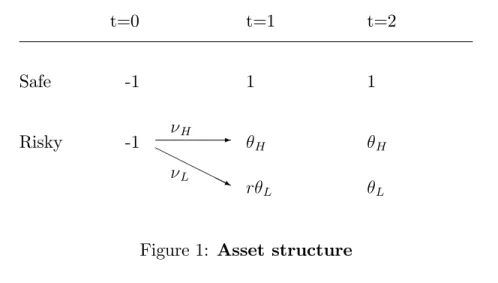
There is a competitive bank that maximizes the expected utility of its depositors. The bank has no endowment but has access to two assets (or technologies): a short-term safe asset and a long-term risky asset. The short-term asset acts like a storage technology: 1 unit invested in this asset in period t yields 1 unit in period t+ 1. The long-term asset is risky and its return depends on the period in which the asset is liquidated and on the state

2 f L; Hg, where Pr ( = j) = j,j =H; L. If the state of the world is , a unit invested

in the long-term asset yieldsr1( ) units if liquidated in period 1or if liquidated in period

2. r1( ) is the early liquidation value of the asset and is given by

r1( ) = 8 < : r L if = L H if = H

5_{Postlewaite and Vives (1987) analyze bank runs when the number of depositors is …nite and liquidity}

t=0 t=1 t=2 Safe -1 1 1 Risky -1 H H r L L -H HH HH_HHj L

Figure 1: Asset structure

where r L < 1 and H > L 1. I assume that E(r1( ))

P

j=L;H jr1( j)< 1 to make

sure that the long-term asset does not dominate the short-term asset. The asset structure is depicted in …gure 1.6

When the state is low, = L, the return of the long-term asset is lower (than in the

high state) if liquidated at maturity and there is a cost of liquidating the long-term asset early, i.e., r <1. In this case, the value of the bank’s assets is low and, as I will show later, depositors have more incentives to withdraw early. Therefore, the bank needs to liquidate more term assets to meet early withdrawals. The costly early liquidation of the long-term asset in the low state captures the idea of a …re sale: when the bank is in distress it sells its assets at a price lower than its value.

In period 0; banks and consumers enter a deposit contract. Following Allen and Gale (1998), the deposit contract allows the consumer to withdraw either cunits at date1or the residue of the bank’s assets at date 2 divided equally among the remaining depositors. If the promised amount c cannot be paid to all early withdrawers, the bank liquidates all its assets and divides the proceeds among those withdrawing early equally. No sequential service 6_{In contrast to Allen and Gale (1998), in which information-based runs can improve risk sharing by}

constraint is imposed, i.e., whether a depositor is the …rst or last to run is irrelevant since all depositors who withdraw early get the same consumption.7 After consumers deposit their endowment but before any uncertainty is revealed, the bank chooses the deposit contract,

c, how much to invest in the long-term asset,L, and how much to invest in the short-term asset, 1 L, to maximize consumers’expected utility.

In period 1, after the depositor type shock has been realized, the state is realized. Depositor i does not observe , but he observes a private signal ei of the return of the

long-term asset where

Pr ei = jj = j =p

1

2 for all i for j =L; H:

Signals are conditionally independent across depositors and each depositor gets a correct signal with probabilityp. The precisionpalso represents the total fraction of depositor who receive the correct signal. In this sense, p can be thought of as a measure of the economy’s transparency. Ifp= 0:5the private signal received by depositoriis not informative: receiving the signal or not does not change his information on the value of the bank’s assets. In this case the bank is opaque: the distribution of information across depositors is independent of the state realized. If p = 1 the private signal is perfectly informative and all depositors observe the value of the bank’s assets after observing the signal. In this sense, whenp= 0:5 the bank is not transparent at all, whereas if p = 1 the bank is completely transparent.8 Depositors use their signaleito learn about the true state using Bayes’s Law. The posterior

7_{This is the same as having a standard deposit contract when banks are competitive. A standard deposit}

contract promises …xed amounts c1 and c2 at periods 1 and 2 respectively and divides all the available resources between withdrawers if the promise cannot be met. Since the bank maximizes depositor’s expected utility, it will never choose to have idle resources in period2and thus whatever the choice ofc2, this promise will never be met. Thus, the contract will reduce to the deposit contract just described.

8_{One can also think of this private signal as having a common component, which captures public}

infor-mation, and an idiosyncratic component captures mistakes people make in processing this information. The appendix formalizes this interpretation of the private signals.

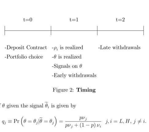
t=0 t=1 t=2 -Deposit Contract -Portfolio choice - _i is realized - is realized -Early withdrawals -Signals on -Late withdrawals Figure 2: Timing

distribution of given the signalei is given by

qj Pr = jje= j =

p j

p j + (1 p) i

j; i=L; H,j ₆=i:

Since p >0:5, the probability of being in state i is higher when the signal is i than when

it is not, i.e., qi >(1 qj) i; j =H; L, j 6=i. For simplicity, I will assume that j = 0:5 so

that qj =p for j = L; H. Finally, after depositors learn their type and their private signal

on , they choose whether to withdraw their funds from the bank in period1or in period2. Figure2 shows the timing.

2.1

Discussion of assumptions

In addition to the information structure, the model described above departs from standard banking models in two ways: risk neutrality for late-consumers and the asset structure. Assuming that late-consumers are risk neutral simpli…es the analysis and makes the model tractable. The asset structure assumed di¤ers from that in Diamond and Dybvig in that there are no liquidation costs when the return of the long-term asset is high. The asset structure in this paper can be thought of as a reduced form of interbank markets, as in Allen et al. (2009), in a one-bank model. In their paper, aggregate shocks to the liquidity demand

a¤ect the price at which banks can sell their long-term assets: periods of high liquidity demand result in …re sales and a low liquidation value, and periods of low liquidity demand in high liquidation value and no discount. Even though this paper abstracts from liquidity shocks (i.e., is …xed), when the return of the long-term asset is low there will be higher incentives for depositors to withdraw early, and in this sense the demand for liquidity will be higher.

3

Optimal Deposit Contract

Consider the problem of a planner who can distinguish early from late consumers and ob-serves the realization of the state ; but is constrained to using the kind of deposit contract described in the previous section. This planner chooses a portfolio,(1 L; L), and a deposit contract, ce_{; c}l_{( ) . He promisesc}e _{to early consumers and givesc}l_{( ) to late consumers in}

state , wherecl_{( ) is the residue of the assets att = 2 divided by the total number of late}

consumers. As described above, ifce _{cannot be paid to all early consumers, all assets would}

be liquidated att= 1 and distributed equally among early consumers. In this case the bank will be bankrupt.9

I will refer to the allocation that arises from choosing the optimal deposit contract as the constrained e¢ cient allocation. Though I am not using the traditional terminology, this allocation is the one chosen by a planner who observes the depositors’ types but is constrained to using deposit contracts.

The planner solves the following problem max

ce_;L E u min c

e_;(1 L) +r1( )L

+ (1 )_E cl( )

9_{Given the asymmetry in the liquidation costs across states, the optimal intermediation contract between}

the bank and the depositors is state contingent. Ifr( H) =r H, deposit contracts would be optimal in this

subject to L ₂ [0;1] 0 ce (1 )cl( ) = 8 < : (1 L) ce_{+ L if c}e _{(1 L)} maxn L ce_r(1 L) 1( ) ;0 o if (1 L)< ce

The …rst constraint states that the planner cannot invest more than the available resources in the long-term asset and that there is no short-selling. The last two sets of constraints are the physical constraints on resources. The amount promised to early consumers has to be non-negative and the amount that is left for late consumers depends on whether the total amount promised to early consumers is less than the liquidity available at t = 1; 1 L. If the planner chooses to give early consumers less than what he invested in the short-term asset, no long-term asset is liquidated early and the available resources at t = 2 are given by (1 L) ce_{+ L. If the planner chooses to give early consumers more than what he}

invested in the short-term asset, some of the long-term asset has to be liquidated early and the available resources at t= 2 are L ce_r(1 L)

1( ) in state .

I will assume that the utility function is such that the constrained e¢ cient contract does not imply bankruptcy for the bank in any state, i.e., ce _{(1 L) +r}

LL. 10

In the terminology of Cooper and Ross (1998), a planner (or bank) chooses to hold excess liquidity if and only if the deposit contract chosen satis…es ce _{<1 L:}

Lemma 1 The planner will choose not to hold excess liquidity. Moreover, the planner will

choose to hold just enough liquidity to pay early consumers, i.e., ce = 1 L:

If ce > 1 L the planner is forced to liquidate some long-term asset early which is not e¢ cient given E[r1( )] <1 < E[ ]. If ce <1 L; the allocation is ine¢ cient since it

10_{To have this it is su¢ cient to assume thatu}0 r L _> (H 1)

allocates too many resources to the short-term asset whose expected payo¤ is less than that of the long-term asset. Therefore, the planner will choose ce= (1 L):

Using the previous lemma, the planner’s problem can be rewritten as follows: max

ce u(c

e_{) +E( ) (1 c}e₎

subject to

ce ₂[0;1]:

Assuming an interior solution, the …rst order condition of this problem is given by

u0(ce ) E( ) = 0: (1)

Since u00<0, this solution is unique. From now on I will assume that ce

2 (0;1) where ce _{is de…ned by (1). Under this}

assumption the constrained e¢ cient allocation is given by

u0(ce ) = E( )

cl ( ) = (1 c

e ₎

1 , = L; H

L = 1 ce ;

Given that the planner observes the true state and each depositor’s type shock i, the

precisionpof the private signal received by depositors does not enter the planner’s problem. The constrained e¢ cient allocation is independent of the precision of information, p, in the economy.

4

Equilibrium

As in any …nite horizon model, the equilibrium can be computed by backward induction. I will start by characterizing the equilibrium of the withdrawal game between depositors

in period 1 taking the bank’s choices of deposit contract and portfolio, (c; L), as given. Then, I will look at the bank’s problem of choosing(c; L)taking into account the depositors’ equilibrium behavior in period 1 for each pair(c; L):

4.1

Withdrawal Game

To solve the withdrawal game between depositors, I will start by characterizing the bene…t of withdrawing early for late consumers. With this in mind, I will show that three regimes may arise depending on the liquidation strategy of the bank when the state is low. Finally, I will show that, for certain choices of the bank, the withdrawal game has multiple equilibria. All early consumers will choose to withdraw in period1since they do not value consump-tion in period 2. Late consumers’ actions will depend on their signal, and on their beliefs on what everyone else’s actions. I will focus on symmetric equilibria of the withdrawal game between consumers in period 1.

De…nition 1 A symmetric equilibrium of the withdrawal game in period 1 is a pro…le =

f L; Hg of withdrawing strategies, where j speci…es the probability with which a late

con-sumer with signal e= j withdraws in period 1 such that, given , each depositor is acting

optimally given his signal.

Given this de…nition of equilibrium, the fraction of depositors who withdraw early in state j given an equilibrium pro…le is

j( ) = + (1 ) (p j + (1 p) i) ; i; j=L; H; j 6=i:

Given the fraction of depositors who withdraw in period 1 in state j; and the contract

and portfolio chosen by the bank in period 0, the bank can be in one of three regimes: no liquidation, partial liquidation, and bankruptcy. In the no liquidation regime, the bank has enough short-term asset to ful…ll all early withdrawals, i.e.,

In the partial liquidation regime, the amount invested in the short-term asset is not enough to cover early withdrawals but all early withdrawals can be met by liquidating some of the long-term asset, i.e.,

1 L < _j( )c 1 L+r1( j)L:

Finally, in the bankruptcy regime the bank cannot meet all early withdrawals even when all of the long-term asset is liquidated, i.e.,

1 L+r1( j)L < j( )c:

4.1.1 Bene…t from withdrawing early

Suppose that depositors observe and that the equilibrium is given by . The bene…t of withdrawing early for a late consumer will depend on the regime and on the equilibrium strategies . As long as the bank is not in the bankruptcy regime, a depositor gets c if he withdraws early and a positive amount if he withdraws at t= 2. If is such that the bank is in the no liquidation regime, the available resources in period2will be given by the return of the long-term asset, L, plus whatever is left in the short-term asset after paying all the depositors who chose to withdraw in period1,1 L _j( )c. In this case, a depositor who withdraws late will receive L+ 1 L _j( )c = 1 _j( ) . In the partial liquidation regime, some of the long-term asset is liquidated to meet the obligations in period 1. Since in period1 the short-term asset is not enough to pay cto all early withdrawers, D units of the long-term asset must be liquidated early. Dis such that the total amount obtained from liquidating the long-term asset is equal to the di¤erence between the amount invested in the short-term asset,1 L, and the amount to be paid in period1, j( )c. Thus, Dis given by

r1( )D= j( )c (1 L);and the only resources left for period2are given by the return

of the unliquidated long-term asset, (L D):Finally, in the bankruptcy regime, all assets are liquidated early and its proceeds are divided equally among early withdrawers, leaving nothing for a depositor who chooses to withdraw late. Therefore, the gain from withdrawing

early rather than late in state j is given by h( j; ) = 8 > > > > > > > > < > > > > > > > > : c jL j( )c+ 1 L 1 _j( ) if j( ) 1 L c c j L j( )c (1 L) r1(1j) 1 _j( ) if 1 L c < j( ) 1 L+r1( j)L c 1 L+r1( j)L j( ) if 1 L+r1( j)L c < j( ):

Lemma 2 h( j; )is increasing in j( )if and only ifr1( j)L+1 L < c <

(1 L+r1( j)L) j( )

.

As the previous Lemma shows, there are strategic complementarities in the withdrawal decision of depositors whenever there is risk sharing and no bankruptcy. If the amount promised to early withdrawers is larger than the minimum return that they would have received if they had invested on the portfolio themselves,i.e., there is no risk sharing, depos-itors have more incentives to withdraw earlier the larger the fraction of earlier withdrawers. In this case, early withdrawers impose an externality on late withdrawers by getting more than their share of the portfolio and decreasing the payo¤ of late withdrawers. This exter-nality will be present as long as the bank is not in the bankruptcy regime. If a late consumer knows that the bank will be bankrupt it is always better for him to withdraw early but, given the pro rata liquidation rule, the bene…t of doing so is decreasing in the amount of depositors who withdraws early.11

Assume that the deposit contract, c, is such that early depositors are promised more than the maximum return on the portfolio,i.e.,c >1 L+ HL:In this case, it is easy to see that

withdrawing early is a dominant strategy for all agents sinceh( H; )>0andh( L; )>0

for all : In the remainder of the paper I will focus on the case in which c 1 L+ HL

which implies the bank is never bankrupt when the high state H is realized. Moreover,

11_{The lack of strategic complementarities in all regimes for all bank choices prevents the equilibrium from}

being unique in the withdrawal game at t = 1 for all possible choices of (c; L): Also, the model does not exhibit one-sided strategic complementarities as in Goldstein and Pauzner (2005).

there is no need to distinguish between the no liquidation and partial liquidation regimes when = H since there are no liquidation costs in this state, i.e., r1( H) = H. Therefore,

the distinction between the no liquidation, partial liquidation, and bankruptcy regime will only apply to the regime that arises in the low state.

Let ( j; ) be the expected bene…t for a late consumer from withdrawing early when

the signal is j and the equilibrium strategy is : Then, given the posterior probability p

and the function h, the expected bene…t is given by

( j; ) ph( j; ) + (1 p)h( i; ) for j; i=L; H; j6=i:

In equilibrium, a late consumer with signal j will choose to withdraw in period 1if and

only if ( j; ) 0; with equality if he chooses to withdraw randomly.

Suppose that p = 1 and that the state was perfectly observed by depositors. If the realized state was H, depositors would have a dominant strategy: all late consumers will

withdraw late regardless of ,h( H; )<0for all , and the equilibrium outcome would be

unique. However, if the state was L, the behavior of late consumers could depend on their

beliefs on the fraction of early withdrawers. In this last case we would be in the Diamond and Dybvig (1983) world and the outcome would depend on which equilibrium is played. If a late consumer believed all other late consumers would withdraw early, he would have incentives to withdraw early. On the other hand, if he expected all other late consumers to wait and withdraw late, he would rather wait to withdraw. These coordination motives would give rise to multiple equilibria of the withdrawal game when the realized state was L.

Therefore, if the state was perfectly observable, coordination motives would only be present in the low state and the incentives of late consumers to withdraw early would always be greater in the low state, i.e., h( H; )< h( L; ).

Now suppose the transparency of the economy decreases and p drops below 1. In this case, keeping the equilibrium strategy pro…le …xed, late consumers with low signals would have lower incentives to withdraw early since now they assign a positive probability to being

in the high state. The withdrawal incentives of late consumers with high signals are a¤ected by two countervailing forces. On the one hand, they have higher incentives to withdraw because they assign a higher probability to the low state occurring. On the other hand, they anticipate that late consumers with low signals have lower incentives to withdraw early which increases the bene…t of withdrawing late in both states. Hence, compared to the case in which signals are perfectly informative, having imperfect information about the state decreases incentives to withdraw early for late consumers with low signals while it may increase or decrease them for those with high signals.

Since depositors with high signals assign a higher probability to being in a high state (in which there are no liquidation costs), if a late consumer with a high signal chooses to withdraw early, then a late consumer with a low signal will choose to withdraw early as well. This is formalized in the following lemma.

Lemma 3 If c < HL+ (1 L), ( H; ) 0 implies ( L; )>0.

As shown in the following corollary, lemma 3narrows down the possible equilibria of the withdrawal game since there cannot be an equilibrium in which some late consumer with high signal withdraws early and some late consumers with low signal does not.

Corollary 1 In equilibrium, L H, with strict inequality if i 2(0;1) i=L; H:

The strategy I follow to compute the equilibria is as follows: I guess that a pair_f L; Hg

among those in corollary 1 is an equilibrium, and then verify conditions on c and L such that the strategy pro…le is indeed an equilibrium. This characterization can be found in the appendix.

4.1.2 Sunspot Equilibria

For every pair(c; L)there exists at least one pro…le that is an equilibrium in the subsequent withdrawal game, but this pro…le may not be unique.

Proposition 1 There exists a nonempty set of deposit contracts, c, and portfolio choices, L, such that the withdrawal game induced by those pairs (c; L) has multiple equilibria.

The proof of this proposition follows from propositions 8; 9; 10; and 11in the appendix. These propositions also characterize the types of multiplicity of equilibria that can arise. For example, they show that for each pair (c; L), there is at most one equilibrium in which the bank is bankrupt.

De…ne byA(c; L)the set of possible equilibria in the withdrawal game given(c; L). The outcome of the game played by the depositors will belong to this set; but, when A(c; L) is not a singleton, it is not possible to predict which equilibria will be played. I assume that the equilibrium that will be played among the elements ofA(c; L)depends on the realization of some exogenous random variable and allow for the probability distribution of this variable to be non degenerate.

De…nition 2 A sunspot equilibrium is a probability density function f : A _! (0;₁) such

that some equilibrium within a set A A is played with probability R_Af(x)dx:

In a sunspot equilibrium, an equilibrium of the withdrawal game is always played and the probability with which it is played depends onf, which can be thought of as the distribution of some observable random variable on which depositors condition their beliefs on how others will behave.

4.2

Bank’s Problem

In what follows I will focus on the bank’s problem in the initial period of the model taking as given the behavior of depositors in the withdrawal game. To de…ne the bank’s objective function, I …rst need to de…ne the bank’s beliefs over how depositors will behave in the withdrawal game for each possible choice of portfolio and deposit contract.

In period0the bank chooses the deposit contract,c, and how much to invest in the short-term and long-short-term assets, (1 L) and L respectively, to maximize depositors’ expected utility taking the depositors’best responses in the withdrawal game as given. The bank is subject to two restrictions: L₂[0;1] and c 0. The …rst restriction simply states that the bank cannot invest more than the resources deposited by consumers and that there is no short-selling. The second constraint places a restriction on the amount that can be o¤ered as part of the deposit contract: depositors have limited liability and therefore cannot be o¤ered negative amounts of c.

4.2.1 Expected Utility

As mentioned above, the withdrawal game may not have a unique equilibrium for some pairs (c; L)_2R+ _{[0;1]. Since the expected utility depends on the fraction of early withdrawers,}

which in turn depends on the equilibrium strategies , I will distinguish between expected utility across equilibria as well as for di¤erent pairs ofcandL. In what follows, I will denote by _{j j}(c; L; ) the fraction of early withdrawers in state j for a given equilibrium

2 A(c; L) and a given pair (c; L). Since and (c; L) determine the regime in which the bank will be, and the amount left for late consumers depends on this regime, it is useful to characterize expected utility under each regime.

No liquidation In the no liquidation regime, Lc 1 L and L2 [0;1]. In this regime,

all early withdrawers get the promised amount c independently of the state . A fraction of the depositors will be early consumers and get utility u(c), while a fraction j of

depositors will be late consumers withdrawing early in state j and will get utility c. In

this region, no long-term asset is liquidated early. Therefore, in state j, the 1 _j late withdrawers each get jL+ 1 L jc = 1 j . Since late withdrawers are always late

consumers, they are risk neutral and therefore the total utility derived from late withdrawers in state j is just jL+ 1 L jc. The expected utility given (c; L)conditional on being in

a no liquidation regime is EUN L(c; L; ) = u(c) + 1 2( L(c; L; ) + H(c; L; ) 2 )c +1 2[( L+ H)L+ 2 (1 L) L(c; L; )c H(c; L; )c] = u(c) c+ 1 2( L+ H)L+ (1 L):

Expected utility in this region does not depend on _Lor _H and it is always increasing in

L sinceE( ) >1: Therefore, conditional on being in the no liquidation region, it is optimal for the bank to invest as much as possible in the long-term asset. In the no liquidation regime expected utility is maximized when Lc= 1 L.

Partial liquidation In the partial liquidation regime, 1 L < _Lc 1 L+r LL and

L ₂ [0;1]. As in the no liquidation regime, early withdrawers always get their promised amount c but some long-term asset must be liquidated to keep this promise. Therefore, in state H there are HL+ 1 L Hc units of the good to divide between (1 H) late

withdrawers, while in state L there are LL+1_r(1 L) 1_r Lcunits of the good to give to

the(1 _L)late withdrawers. Expected utility in a partial liquidation regime is given by

EUP L(c; L; ) = u(c) + 1 2( L(c; L; ) + H(c; L; ) 2 )c +1 2 LL+ 1 r (1 L) 1 r L(c; L; )c+ HL+ 1 L H(c; L; )c :

The derivative of the objective function with respect to L is given by

@EUP L @L = 1 2 @ _L(c; L; ) @L 1 1 r c+ 1 2( L+ H) 1 2 1 + 1 r : Thus, if @ L( ;c;L)

@L = 0; the bank will choose Lc= 1 L.

Bankruptcy If the bank is in the bankruptcy regime in the low state, 1 L+r LL < Lc and L 2 [0;1]. In this regime the bank cannot pay the promised amount c to early

withdrawers in state Land thus liquidates all the long-term asset early, leaving nothing for

late withdrawers when = L. Therefore, in the low state, which occurs with probability0:5,

all early withdrawers get r LL+1 L

L units of the good. Early consumers value itu

r LL+1 L L

and L late consumers value it

r LL+1 L

L . The(1 L)late withdrawers get0utility. In

the high state, the bank is able to pay the promised amountc to the _H early withdrawers ( early consumers) and gives out HL+ (1 L) Hcto the(1 H)late withdrawers (all

late consumers). Expected utility in this region is given by

EUB(c; L; ) = 2u(c) + 2u r LL+ 1 L L(c; L; ) +1 2( L ) r LL+ 1 L L(c; L; ) +1 2( )c+ 1 2( HL+ (1 L)):

4.3

Equilibrium

Using the expressions for expected utility derived in the previous subsection, expected utility as a function of the equilibrium , and of the bank’s choices(c; L), is given by

EU(c; L; ) = 8 > > > < > > > : EUN L_{(c; L; ) if} L(c; L; )c 1 L EUP L_{(c; L; ) if 1 L <} L(c; L; )c 1 L+r LL EUB_{(c; L; ) if 1 L+r} LL < L(c; L; )c:

Since the bank maximizes the depositors’expected utility, the bank’s choices potentially depend on its beliefs over how depositors will coordinate on equilibria, i.e., on the sunspot equilibrium the bank anticipates depositors will play. For example, the bank can be opti-mistic and think that depositors will always coordinate in the Pareto dominant equilibrium. Alternatively, it can be pessimistic and assume that depositors will coordinate on the worst equilibrium possible. The bank´s beliefs may also be equal to any other probability distrib-ution over these equilibria and any other equilibrium that can occur.

Recall that A(c; L) is the set of all strategy pro…les that are equilibria in the with-drawing game given(c; L).

De…nition 3 A set of beliefs for the bank is a probability density function (c;L) :A(c; L)!

[0;+₁) for each pair (c; L)_{2 R}+ _[0;1]:

IfA(c; L)is not a singleton there is a continuum of possible functions (c;L), and therefore,

there are many possible sets of beliefs for the bank. Given a set of beliefs , the bank chooses (c; L) to maximize depositors’ expected utility and, therefore, the choice of (c; L) might depend on the set of beliefs the bank has.

De…nition 4 An equilibrium in this model is a pair (co_{; L}o₎

2 R+ _{[0;1], beliefs for the}

bank, , and a probability density function over A(co_{; L}o_{), f, such that:}

(i) (co_{; L}o_{) solves} max (c;L)2R+ _[0;1] Z A(c;L) (c;L)( )EU(c; L; )d ;

(ii) f is a sunspot equilibrium in the withdrawal game induced by (co_{; L}o_{); and}

(iii) f = (co_;Lo₎.

Condition (i) requires that (co_{; L}o_{) solve the bank’s problem given the set of beliefs}

. Condition (ii) requires that an equilibrium is played in the withdrawal game. Finally, condition (iii) imposes consistency between the bank’s beliefs and the sunspot equilibrium played by depositors in the withdrawal game induced by (c0_{; L}0_).

5

Fragility

The constrained e¢ cient allocation can only be attained in an equilibrium in which only early consumers withdraw at t = 1. Otherwise, since ce _{= 1 L , some of the long-term asset}

would need to be liquidated early to pay all early withdrawers and cl₍

L) < cl ( L): This

implies that to achieve the constrained e¢ cient allocation in a decentralized equilibrium, the constrained e¢ cient allocation has to be incentive compatible, i.e., late consumers have to be willing to wait and withdraw in the second period for whatever signal they get.

De…nition 5 An allocation (c1; c2( )) is incentive compatible i¤

c1 Ep(c2( )j i) for i=L; H: (2)

where _Ep(c2( )j i) = pc2( i) + (1 p)c2( j), i; j =L; H, i6=j.

The set of incentive compatible allocations depends on the level of transparency of the economy, p, through the expectation operator _Ep. Moreover, the more transparent the

economy the smaller the set of incentive compatible allocations. It is easier to satisfy an ex-ante incentive compatibility constraint than state by state ones. When p = 0:5, private signals do not reveal any new information to depositors and an allocation needs to satisfy a unique ex-ante incentive compatibility constraint to be incentive compatible. As the level of transparency increases, the conditions in(2) resemble state by state incentive compatibility constraints more and more, reducing the set of incentive compatible allocations.

Proposition 2 The constrained e¢ cient allocation is incentive compatible if and only if

p H(1 c

e _{) (1 )c}e

( H L) (1 ce ) b

p:

Proposition2states that if the precision of the private signal is low enough (p p_b) there exists an equilibrium in the withdrawal game given (ce _{; L ) in which only early consumers}

withdraw early, and, therefore, the constrained e¢ cient allocation can be achieved in a decentralized equilibrium. The constrained e¢ cient welfare can only be attained in economies in which transparency is low. This, however, does not imply that the constrained e¢ cient welfare will always be attained: in order to strictly implement the constrained e¢ cient allocation it must be the case that there is a unique equilibrium in the withdrawal game induced by (ce _{; L ).}

There are many de…nitions of fragility in the banking literature. I will follow Keister (2012) and say that the economy is fragile if there is an equilibrium in which some late consumers withdraw early, i.e., when a bank run (partial or total) in some state is part of an equilibrium in the withdrawal game.

De…nition 6 The economy is fragile if for some equilibrium of the model (c; L; ;f) there exists an equilibrium in the subsequent withdrawal game in which some late consumers with-draw early with positive probability.

The de…nition of fragility presented in this section says that if, for all sets of equilibrium beliefs , the bank chooses a pair (c; L) such that the equilibrium of the withdrawal game is unique and no late consumers withdraw early in it, then the economy is not fragile. If the economy is not fragile, a solvent bank is not susceptible to bank runs and there are no expectation-driven equilibria.

In terms of fragility, for the constrained e¢ cient allocation to be attained for any set of beliefs for the bank, (ce _{; L ) has to be incentive compatible in an economy that is not}

fragile. As the following proposition shows, this will be the case when transparency is low enough.

Proposition 3 There exists p p^₂ (0:5;1) such that the bank chooses (ce _{; L ) (for all}

possible beliefs ) and the economy is not fragile if and only if p < p .

When p < p , the constrained e¢ cient allocation is the unique equilibrium allocation of the model. For all possible beliefs , the bank chooses (ce _{; L ) and only early consumers}

withdraw early in the subsequent withdrawal game, i.e., A(ce ; L ) = _f =_f0;0_gg. Con-sider the withdrawal game given (ce _{; L ) and suppose p >^ 0:5. Recall from section 4 that}

coordination motives are only present when the state is low. As discussed above, the absence of liquidation costs in the high state implies that if depositors could observe the state per-fectly they would always have a dominant strategy, and the equilibrium would be unique if the high state was realized. In particular, ifc < HL+ (1 L)late-consumers would always

choose to withdraw late if they observed H. When signals are not perfectly informative,

depositors will make their withdrawal decision contingent on their information, weighting the expected gains and losses from their action in both states of the world. If late-consumers

with low signals assign enough weight to the high state, they will choose not to run regardless of the actions of others, and the equilibrium of the withdrawal game will be unique. This happens when p < p .

When p > p late consumers with low signals assign enough probability to the low state happening such that coordination motives become relevant. In this case, incentives to withdraw early become stronger and may even lead to late consumers with high signals withdrawing early. On one hand, an increase in the transparency level, p, increases the weight late-consumers with high signals assign to the high state. This e¤ect decreases their incentives to run. On the other hand, when p > p , late-consumers with low signals have more incentives to run which may lead to larger losses of waiting to withdraw if the low state is realized. This e¤ect increases the incentives to withdraw early. Whether late-consumers with high signals withdraw early will depend on which of these two e¤ects is stronger, which in turn depends on their beliefs about what other depositors will do. In any event, increasing the precision of information abovep gives rise to coordination motives that would otherwise be inexistent, and may prevent the constrained e¢ cient level of welfare from being attained. Assume a planner who cannot control the bank’s beliefs over what depositors will do, nor which equilibrium depositors will play. Then, from this planner’s point of view, the safest transparency level would be some p < p . If p < p , the equilibrium allocation is guaranteed to be constrained e¢ cient and the probability of bank runs is0. Any other level of transparency is risky since the equilibrium played may involve bank runs and, therefore, expected utility may be below the constrained e¢ cient level. Increasing information on the value of the bank’s assets can decrease the maximum level of expected utility that can be attained in equilibria but it may also make the economy fragile. If this was the case, even if the constrained e¢ cient allocation was attainable it might not be attained in equilibrium.12

5.1

Fragility and Liquidation Costs

As in the standard Diamond and Dybvig model, the strategic complementarities in the with-drawal game arise from the liquidation costs in the low state. As discussed in section2:1, the asset structure captures the …re sales that occur when banks are forced to sell a large fraction of their assets. These …re sales are not unique to the banking industry. Whenever there is a maturity mismatch between the assets and liabilities held by the …nancial intermediaries, as is the case for money market funds and mutual funds, there is potential for strategic complementarities to arise (Chen et al. (2010) show evidence of these complementarities). Especially if one considers that the redemption of liabilities can imply the liquidation of long term assets at …re sale prices. In sum, the strategic complementarities described in the paper can be present whenever there are liquidation costs associated with meeting the redemption of short term liabilities.

As the following proposition shows, the larger the liquidation costs, the stronger the depositors’ incentives to coordinate and the larger the strategic complementarities. These stronger strategic complementarities imply that it is harder to support the constraint e¢ cient allocation as the unique equilibrium: the set of transparency levels such that second best e¢ ciency is attained shrinks with the liquidation cost of the asset. Moreover, the likelihood that the economy is fragile for a given transparency level increases with the liquidation cost.

Proposition 4 The threshold p is increasing in r.

The proof follows from the characterization of p in the appendix using the implicit function theorem.

5.2

Optimistic Bank

To illustrate the e¤ects of transparency on the bank’s portfolio choices, I focus on an opti-mistic bank. However, all the results will hold qualitatively if a bank held other beliefs.

Assume that the bank is optimistic, that is, that for any deposit contract and portfolio in the bank’s choice set such that there are multiple equilibria, the bank thinks that depositors will coordinate on the Pareto-dominant equilibrium. In order to characterize the choice of an optimistic bank, one needs to characterize the optimistic bank’s beliefs by ranking the possible equilibria for each pair (c; L).

For a given pair (c; L) there may be two di¤erent types of multiplicity: within the same regime and across regimes. The following propositions ranks equilibria within the same regime and across regimes.

Proposition 5 Take a pair (c; L) in which there are multiple equilibria within the same regime. Then, expected utility is (weakly) higher in the equilibrium with the lowest fraction of early withdrawers.

Proposition 6 For a given pair (c; L)

EUN L c; L; N L >max EUP L c; L; P L ; EUB c; L; B

where j is any withdrawing strategy such that, given (c; L) the bank is in regime j in the

low state.

In the no liquidation regime no long term asset is liquidated early and all early withdraw-ers get the promised amount. Convwithdraw-ersely, in the partial liquidation and bankruptcy regimes some or all of the long term asset is liquidated early and early withdrawers might get less than what they were promised. Hence, expected utility is higher under the no liquidation regime.

With these propositions in mind, and using the characterization of equilibria in the appendix, one can characterize the beliefs of an optimistic bank. These are depicted in …gure 3. For those pairs (c; L) in region 1, the Pareto-dominant equilibrium is a no run equilibrium. If the no run equilibrium will be played, the bank will be in the no liquidation

regime in region 1a, in the partial liquidation regime in region 1b, and in region 1c the bank will be bankrupt if the low state is realized. In region 2, an optimistic bank assigns probability1to the equilibrium in which all late consumers with low signals withdraw early. In region 2a, the amount of liquidity held by the bank, 1 L, is enough to pay all early withdrawers without liquidating any long term asset (no liquidation regime). In region 2b, the bank will be in the partial liquidation regime if the low state is realized and the best equilibrium is played. In region 3, the Pareto-dominant equilibrium is such that the bank will be bankrupt if the low state is realized. Finally, in region 4, c > HL+ (1 L) and

withdrawing early is a dominant strategy for all depositors.

As Cooper and Ross (1998), and Ennis and Keister (2006) point out there are two reasons why a bank may choose to hold excess liquidity when the liquidation of long term assets is costly. Holding liquid assets minimizes the liquidation costs if a run were to occur; and it may decrease the incentives of late consumers to run.13

If the bank chooses to be in the no liquidation region, then he will always choose Lc=

(1 L). Otherwise, he could always increase expected welfare by increasing Lsince _E( )>

1. In the partial liquidation region, if L is …xed, a bank will always choose Lc= (1 L):

In this case, it is too costly to liquidate long term assets to pay late consumers who withdraw early: for each unit of consumption paid to a late consumer withdrawing early in the low state, late consumers withdrawing late would lose 1=r . Suppose that _Lc > (1 L):Then, by increasing the amount of short term asset by , late consumers would lose ( H 1)

in the high state but they would gain 1

r L in the low state. Since E(r( )) <1, the

bank would be better o¤ decreasingL and choosing Lc= (1 L).

If a bank chooses to avoid bankruptcy, he will only hold excess liquidity if he expects a partial run to occur in the low state. In this case, having some excess liquidity (i.e., 13_{In constrast to Cooper and Ross (1998), and Ennis and Keister (2006) I do not allow for multiple}

equilibria in my analysis in this section. I focus on the best equilibrium being played. Nevertheless, the occurrence of bank runs is random and depends on the low state being realized.

Figure 3: Beliefs of an optimistic bank. The best equilibrium in region 1 is a no-run equilibrium. The bank will be in the NL regime in region 1a, in the PL in region 1b, and in the bankruptcy regime in region1c: In region 2, the best equilibrium is the one in which only late consumers with low signals withdraw early. In region 2a the bank will be in the NL regime and in region 2b in the PL regime. In region 3 the best equilibrium implies the bank will be bankrupt if the low state is realized. Finally, in region 4, withdrawing early is a dominant strategy for all depositors since c > LL+ (1 L):

c < 1 L) helps the bank avoid liquidation costs in the event of a run, and deters late consumers with high signals from withdrawing early. If a bank chooses to be in a no-run region and avoid bankruptcy, he will not hold any excess liquidity.14

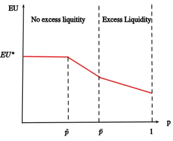
Proposition 7 There exists a threshold p >p^such that for all p₂ 1₂; p an optimistic bank chooses an allocation that is run-proof and holds no excess liquidity in equilibrium.

The proof of this proposition follows from lemmas 4 and 5, and the characterization of equilibria in the appendix. Suppose that a bank always chooses to avoid bankruptcy. Then, the decision to hold excess liquidity in equilibrium, will depend on the transparency level of the economy. When p < p^, the constrained e¢ cient level of welfare can be attained in equilibrium and the bank will not hold excess liquidity. For transparency levels higher than ^

p, the constrained e¢ cient allocation is no longer incentive compatible and the maximum expected utility that can be attained is less thanEU . If p₂(^p; p), the bank chooses a no-run equilibrium and does not hold excess liquidity. Forp > p, preventing bank runs becomes too costly in terms of forgone risk sharing: the amount of consumption that needs to be promised to early withdrawers that deters late consumers with low signals from withdrawing early is too low. In this case, the bank is better o¤ choosing a pair (c; L) in the partial run region and giving early consumers a higher consumption.15

The choices of this optimistic bank give an upper bound to the expected utility that can be attained in equilibrium for di¤erent transparency levels. Figure 4 shows the supremum for the set of attainable expected utility in equilibrium.

14_{Ennis and Keister (2006) …nd that, in a model with liquidation costs and without uncertainty, depositors}

with preferences given by c = ; ₂(0;1), a bank will never hold excess liquidity to mitigate the e¤ects of a potential run. Ratnovski (2013) analyzes transparency as a substitute to liquidity holdings.

15_{These qualitative results do not depend on the bank being optimistic. The incentives of non optimisitc}

Figure 4: Maximum attainable expected utility in equilibrium.

6

Conclusion

There are many dimensions in which a …nancial institution can be transparent. For example, banks can be transparent about their liquidity holdings, their capital structure, and even the of stress tests. In this paper I highlight a novel channel through which transparency can be costly for …nancial institutions by focusing on the transparency about the value of assets. In the presence of strategic complementarities, increasing the precision of the private information depositors have about the value of the assets of a bank decreases welfare by reducing the amount of risk sharing in the economy and by increasing the bank’s vulnerability to runs.

When the transparency level is low, depositors cannot distinguish low states from high states based on their own signals, and, unless they are hit with a liquidity shock, they have few incentives to withdraw early. In this case, they do not act on their information and there are no bank runs in equilibrium. As the transparency level increases, the private signals become more informative and the incentives to withdraw early become stronger, giving rise to equilibria with bank runs. As transparency and coordination motives increase, the set

of incentive compatible allocations from which the bank can choose shrinks and it becomes costlier for the bank to choose a portfolio and a deposit contract such that there will be no runs. For low enough levels of transparency the second best allocation is attained in equilibrium. However, when transparency is high enough, the bank chooses to hold excess liquidity and forgo return in order to deter some depositors from running and to minimize the costs of ine¢ cient bank runs.

The mechanism described in the paper relies on the strategic complementarities that arise in the model due to the maturity mismatch between assets and liabilities and on the liquidation costs implied by the early liquidation of long term assets. This feature is not unique to banks: the mechanism is also particularly relevant for intermediaries that hold assets for which there are no market quotations and in which the liquidation of assets is costly, such as money market funds and some open-ended mutual funds. These …nancial intermediaries hold portfolios that are not perfectly liquid and their shareholders can redeem their shares on demand daily. In fact, the asset classes in which money market funds trade are usually subject to …re sales if not held to maturity. As the paper shows, increasing transparency about the value of the assets held by these …nancial intermediaries can increase the coordination motives between investors and, thus, these institutions’ vulnerability to runs.

References

Acharya, Viral and Tanju Yorulmazer (2008), “Information contagion and bank herding.”

Journal of Money, Credit and Banking, 40(1), 215½U231.

Allen, Franklin, Elena Carletti, and Douglas Gale (2009), “Interbank market liquidity and central bank intervention.”Journal of Monetary Economics, 56, 639–652.

Allen, Franklin and Douglas Gale (1998), “Optimal …nancial crises.”Journal of Finance, 53, 1245–1284.

Basel Committee on Banking Supervision (June 2012), “Composition of capital disclosure requirements.”http://www.bis.org/publ/bcbs221.pdf.

Bouvard, Matthieu, Pierre Chaigneau, and Adolfo" "de Motta (2014), “Transparency in the …nancial system: Rollover risk and crises.”working paper.

Calomiris, Charles W. and Charles M. Kahn (1991), “The role of demandable debt in struc-turing optimal banking arrangements.”American Economics Review, 81, 497–513.

Chari, V.V. and Ravi Jagannathan (1988), “Banking panics, information, and rational expec-tations equilibrium.”The Journal of Finance, 42, 749–761.

Chen, Qi, Itay Goldstein, and Wei Jiang (2010), “Payo¤ complementarities and …nancial fragility: Evidence from mutual fund out‡ows.”Journal of Financial Economics, 97, 239– 262.

Chen, Yehning and Iftekhar Hasan (2006), “The transparency of the banking system and the e¢ ciency of information-based bank runs.”Journal of Financial Intermediation, 9, 240–273. Cooper, Russell and Thomas Ross (1998), “Bank runs: Liquidity costs and investment

distor-tions.”Journal of Monetary Economics, 41, 27–38.

Diamond, Douglas W. and Philip H. Dybvig (1983), “Bank runs, deposit insurance, and liq-uidity.”Journal of Political Economy, 91, 401–419.

Ennis, Huberto M. and Todd Keister (2006), “Bank runs and investment decisions revisited.”

Journal of Monetary Economics, 53, 217½U232.

Goldstein, Itay and Yaron Leitner (2013), “Stress tests and information disclosure.”Working

Goldstein, Itay and Ady Pauzner (2005), “Demand deposit contracts and the probability of bank runs.”Journal of Finance, 60, 1293–1327.

Goldstein, Itay and Haresh Sapra (March 2014), “Should banksŠ stress test results be disclosed? an analysis of the costs and bene…ts.”Foundations and Trends in Finance, 8, 1–54.

Hirshleifer, J. (1971), “The private and social value of information and the reward to inventive activity.”American Economic Review, 61, 561½U574.

Iachan, Felipe S. and Plamen T. Nenov (forthcoming), “Information quality and crises in regime-change games.”Journal of Economic Theory.

Keister, Todd (2012), “Bailouts and fragility.”Federal Reserve Bank of New York Sta¤ Reports, 473.

Landier, Augustin and David Thesmar (2011), “Regulating systemic risk through transparency: Tradeo¤s in making data public.”working paper, NBER.

Leitner, Yaron (2014), “Should regulators reveal information about banks?” Federal Reserve

Bank of Philadelphia Business Review Articles, Third Quarter.

Lopez, Jose A. (2003), “Disclosure as a supervisory tool: Pillar 3 of basel ii.”FRBSF

ECO-NOMIC LETTER, 22.

Morris, Stephen and Hyun Song Shin (2002), “Measuring strategic uncertainty.”Pompeu Fabra workshop on "Coordination, Incomplete Information, and Iterated Dominance: Theory and

Empirics", August 18-19.

Postlewaite, Andrew and Xavier Vives (1987), “Bank runs as an equilibrium phenomenon.”

Journal of Political Economy, 95, 485–491.

Ratnovski, Lev (2013), “Liquidity and transparency in bank risk management.”Journal of

Yorulmazer, Tanju (2003), “Herd behavior, bank runs and information disclosure.”working

7

Appendix

7.1

Private signals and public information

eh =v+sh

where v _{2 f} H; Lg with Pr (v = ij = i) = pv and sh_i 2 f0; j vg with

Pr sh

i = 0jv = i = ps > 0:5. v is the common component of the private signals and

can be interpreted as public information. sh is an idiosyncratic shock and it implies some people will make mistakes even after observing the signal v. Then,

Pr eh = ij = i = Pr v = i; sh = 0j = i + Pr v = j; sh = i jj = i

= pvps+ (1 pv) (1 ps)

Letp:=pvps+ (1 pv) (1 ps). Then, an increase in the precision of public information pv

translates directly to an increase in the precision of the private signalp.

7.2

Constrained e¢ cient allocation

Lemma 1 The planner will choose not to hold excess liquidity. Moreover, the planner will choose to hold just enough liquidity to pay early consumers, i.e., ce _{= 1 L:}

Proof. Recall thatE( ) > 1 and r L < 1, H 1 +r L_r 1 <0. Suppose that ce >1 L.

In this case, the planner could increase welfare by decreasing L. Since H 1 +r L_r 1 <0,

decreasingLwould increase the amount of expected resources available att= 2and expected welfare. Alternatively, if ce _{< 1 L, the planner could increase the objective function by}

increasing L. Since E( ) >1, increasing L would increase the expected resources available in period 2 and therefore increase aggregate expected welfare.

7.3

Bene…t from withdrawing early

Lemma 3 If c < HL+ (1 L), ( H; ) 0 implies ( L; )>0.

Proof. When c < HL+ (1 L), h( H; ) < 0 for all . Then, if ( H; ) 0 it must

be that h( L; )>0. Since p > 1₂, ( L; ) puts more weight on h( L; ) than h( H; ).

Therefore, if ( H; ) 0 it must be the case that ( L; )>0.

Corollary 2 1 In equilibrium, L H, with strict inequality if i 2(0;1) i= 1;2:

Proof.To have L2(0;1)and H 2(0;1) in equilibrium it must be that

( H;f L; Hg) = 0 and ( L;f L; Hg) = 0: (3)

But from the lemma I know that ( H;f L; Hg) = 0 implies ( L;f L; Hg)>0.

There-fore,(3) can never hold.

Assume L< H in equilibrium. From the …rst part of this proof, only two cases are possible:

(i) L = 0and H 2(0;1]; and(ii) L= [0;1)and H = 1. To be in case(i)it must be the

case that ( H;f L; Hg) = 0 and ( L;f L; Hg)<0 which contradicts the lemma. For

case(ii) ( H;f L; Hg)>0and ( L;f L; Hg) = 0have to hold, which also contradicts

the lemma. Then, there can’t be an equilibrium in which L< H:

Finally, from the …rst part of this proof, if L = H = it must be that 2 f0;1g.

7.4

Equilibrium determination

I will only consider(c; L)_2R+ _{[0;1]but I will omit this for notation simplicity. LetW}R_be

the set of all pairs(c; L)such that is an equilibrium in regimeR in the withdrawing game. Corollary1shows that there can be …ve di¤erent kinds of equilibria in the withdrawal game: (1) L= H = 1 and ( L;f1;1g) 0and ( H;f1;1g) 0, (2) L = 1,1> H >0and

( L;f1; Hg) 0and ( H;f1; Hg) = 0,(3) L= 1, H = 0and ( L;f1;0g) 0and

( H;f1;0g) 0,(4) 1> L>0, H = 0and ( L;f L;0g) = 0and ( H;f L;0g) 0,

7.4.1 Everybody withdraws early

If L = H = 1 is an equilibrium, I must have ( H;f1;1g) 0. This means, that L = H = 1can only be an equilibrium whenc 1 L+R H. Ifc <1 L+R H, ( H;f1;1g) =

1. Since there is always something left to withdraw in the second period even if everyone chooses to withdraw in the …rst one, and each consumer has measure 0, the bene…t of withdrawing early in this case is negative and equal to ₁: Moreover, I know that if c

1 L+R H withdrawing early is a dominant strategy. Therefore, in this region there is a

unique equilibrium. If L = H = 1is an equilibrium I have bankruptcy in both states. From

now on consider the case in whichc < 1 L+R H. In this area there is never bankruptcy

in the high state.

7.4.2 No late consumer withdraws early

To have L = H = 0 an equilibrium I must have ( ;f0;0g) <0 for = L; H, i.e., the

expected bene…t of withdrawing early has to be negative for any signal received.

From Lemma 1, I know that ( L;f0;0g) 0 implies ( H;f0;0g) < 0. Therefore it is

enough to …nd all(c; L)such that ( L;f0;0g) 0:

There are 3 cases: 1. No liquidation c p( LL+ (1 L) c) 1 (1 p) ( H + (1 L) c) 1 0 which gives c L(p L+ (1 p) H) + (1 L) and WN L f0;0g =f(c; L) :c L(p L+ (1 p) H) + (1 L) and c (1 L)g: 2. Partial Liquidation c p L L+ [(1 L) c]_r1_L 1 (1 p) ( H + (1 L) c) 1 0

or rewriting this expression c (p L+ (1 p) H)L+ (1 L) p 1 r + (1 p) 1 1 p1_r + (1 p) : Then, W_fP L_0;0g = (c; L) :c (p L+(1 p) H)L+(1 L)(p 1 r+(1 p)) (1 ₍1 ₍p1_r+(1 p)₎₎₎ and 1 L < c <1 L+r LL : 3. Bankruptcy p1 L+r LL+ (1 p) c ( H + (1 L) c) 1 0 or c ( H + (1 L)) p (1 p) (1 ) (1 L+r LL): Thus,W_fB_0;0g = n (c; L) :c ( H+(1 L) c) 1 p (1 p) 1 L+r LL _{and c 1 L+r} LL o :

7.4.3 Only late consumers with low signals withdraw

There are 2 cases in which only late consumers with low signals withdraw early: they can be indi¤erent between doing so and waiting or they might strictly prefer it.

To have L2(0;1) H = 0 an equilibrium it must be that

( L;f L;0g) = 0 and ( H;f L;0g)<0:

From lemma 1it is enough to check that ( L;f L;0g) = 0.

1. No liquidation

c=p LL+ (1 L) Lc

1 _L + (1 p)

HL+ (1 L) Hc

1 _H :

Using the de…nition of L

c= p L(1 (1 p) L) + (1 p) H(1 p L) (1 2p L(1 p))

The right hand side of this equality is decreasing in L and if( + (1 )p L)c < 1 L, c <(1 L):Therefore, W_fN L L;0g = 8 < : (c; L) :c= p L(1 (1 p) L)+(1 p) H(1 p L) (1 2p L(1 p)) L+ (1 L) and ( + (1 )p L)c <1 L 9 = ; and W_fN L L;0g W N L f0;0g. 2. Partial liquidation c=p LL+ 1 r(1 L) 1 r Lc 1 _L + (1 p) HL+ (1 L) Hc 1 _H :

Using the de…nition of L and H

c= (p L(1 H)+(1 p) H(1 L))L+[(1 )+(1r 1)p ( 1 r+1)p(1 p) L](1 L) (1 )(1+(1_r 1)p (1 L) (1_r 1)(1 )(1 p)p2 2L p(2 p(1+ 1 r)) L) (4) Therefore, W_fP L L;0g =f(c; L) : (4) holds and 1 L < Lc <1 L+r LLg

Moreover, it can be show that

D [ L2[0;1] WP L f L;0g = (c; L) :c (1 p) (1 (2p 1))((r L+ H)L+ 2 (1 L)) \ (c; L) :c ((1 )(p 2 L+(1 p)2 H)L+((1 )+(1_r 1)p (1_r+1)(1 p)p)(1 L)) ((1 )(1 (1_r 1)(1 )(1 p)p2 _{p(2 p(1+}1 r)))) \ (c; L) :c (( H+ L)L+( 1 r+1)(1 L)) ((1 )(1 p)₍1 _r1₎+₍1+1_r)) \ f(c; L) :c _bc(L)_g where _bc(L) is de…ned by:

b c(L) 0 @ (2 (1 p) (1 + ) + (1 )) (1 L) + ( E( ) 2 (1 p) + (1 ) (p L+ (1 p) H))L 1 A = (1 L) (2 (1 p) (1 +L(E( ) 1))) +c_b(L)2(2 (1 p) + (1 )): (5)

3. Bankruptcy

pr LL+ (1 L)

L

+ (1 p) c HL+ (1 L) Hc

1 _H = 0

which can be rewritten as

c= HL+ (1 L) p(1 _H) (1 p) _L (r LL+ (1 L)): Thus, W_fB L;0g = (c; L) :c= HL+ (1 L) p(1 _H) (1 p) _L (r LL+ (1 L)) and Lc 1 L+r LL :

It can be shown that

D [ L2[0;1] W_fB L;0g = (c; L) :c (1 p) 1 (2p 1)(( H + Lr)L+ 2 (1 L)) \ (c; L) :c ( HL+ 1 L) (1 )p (1 p) (r LL+ 1 L) \ (c; L) :c ( HL+ 1 L) p2(1 ) (1 p) ((1 )p+ )(r LL+ 1 L) :

To have L= 1 H = 0 in equilibrium it must be that

( L;f1;0g)>0> ( H;f1;0g): 1. No liquidation c 1 2[ L+ H]L+ (1 L) and c p 2 L+ (1 p) 2 H (1 2p(1 p)) ! L+ (1 L):