SFB 649 Discussion Paper 2010-003
Uniform confidence
bands for pricing kernels
Wolfgang Karl Härdle*
Yarema Okhrin**
Weining Wang*
* Humboldt-Universität zu Berlin, Germany ** Universität Augsburg, Germany
This research was supported by the Deutsche
Forschungsgemeinschaft through the SFB 649 "Economic Risk". http://sfb649.wiwi.hu-berlin.de
ISSN 1860-5664
SFB 649, Humboldt-Universität zu Berlin Spandauer Straße 1, D-10178 Berlin
S
FB
6
4
9
E
C
O
N
O
M
I
C
R
I
S
K
B
E
R
L
I
N
Uniform confidence bands for pricing kernels
∗
Wolfgang Karl H¨
ardle
†,Yarema Okhrin
‡, Weining Wang
§.
Abstract
Pricing kernels implicit in option prices play a key role in assessing the risk aversion over equity returns. We deal with nonparametric estimation of the pricing kernel (Empirical Pricing Kernel) given by the ratio of the risk-neutral density esti-mator and the subjective density estiesti-mator. The former density can be represented as the second derivative w.r.t. the European call option price function, which we estimate by nonparametric regression. The subjective density is estimated nonpara-metrically too. In this framework, we develop the asymptotic distribution theory
of the EPK in the L∞ sense. Particularly, to evaluate the overall variation of the
pricing kernel, we develop a uniform confidence band of the EPK. Furthermore, as an alternative to the asymptotic approach, we propose a bootstrap confidence band. The developed theory is helpful for testing parametric specifications of pricing ker-nels and has a direct extension to estimating risk aversion patterns. The established results are assessed and compared in a Monte-Carlo study. As a real application, we test risk aversion over time induced by the EPK.
Keywords: Empirical Pricing Kernel; Confidence band; Bootstrap; Kernel
Smooth-ing; Nonparametric FittingJEL classification: C00; C14; J01; J31
1
Introduction
A challenging task in financial econometrics is to understand investors’ attitude towards market risk in its evolution over time. Such a study naturally involves stochastic discount factors, empirical pricing kernels (EPK) and state price densities, see Cochrane (2001). Asset pricing kernels summarize investors’ risk preferences and exhibit when estimated from data, the so called “EPK paradox”, as several studies including A¨ıt-Sahalia and Lo (2000), Brown and Jackwerth (2004), Rosenberg and Engle (2002) have shown. Although in all these studies the EPK paradox (non-monotonicity) became evident, a test for the
∗The financial support from the Deutsche Forschungsgemeinschaft via SFB 649 “ ¨Okonomisches
Risiko”, Humboldt-Universit¨at zu Berlin is gratefully acknowledged.
†Professor at Humboldt-Universit¨at zu Berlin and Director of CASE - Center for Applied Statistics and
Economics, Humboldt-Universit¨at zu Berlin, Spandauer Straße 1, 10178 Berlin, Germany and National
Central University, Department of Finance, No. 300, Jhongda Rd., Jhongli City, Taoyuan County 32001, Taiwan (R.O.C.). Email:[email protected]
‡Professor at University of Augsburg, Department of Statistics, Universitaetsstraße 16, D-86159
Augs-burg, Germany. Email:[email protected]
§Corresponding author. Research associate at Ladislaus von Bortkiewicz Chair, the Institute for
Statistics and Econometrics of Humboldt-Universit¨at zu Berlin, Spandauer Straße 1, 10178 Berlin,
functional form of the pricing kernel has not been devised yet. A uniform confidence band drawn around an EPK is a very simple tool for shape inspection. Confidence bands based on asymptotic theory and bootstrap is the subject of our paper. In addition, we relate critical values of our test to changing market conditions given by exogenous time series. The common difficulty is that the investors’ preference is implicit in the goods traded in the market and thus can not be directly observed from the path of returns. A profound martingale based pricing theory provides us one approach to attack the problem from a probabilistic perspective. An important concept involved is the State Price Density (SPD) or Arrow-Debreu prices reflecting fair prices of one unit gain or loss for the whole market. Under no arbitrage assumption, there exists at least one SPD, and when a market is complete, there is a unique SPD. Assuming markets are complete, pricing is done under a risk neutral measure, which is related to the pdf of the historical measure by multiplying with a stochastic discount factor, see section 2 for a detailed illustration. From an economic perspective, the price is formulated according to utility maximization theory, which admits that the risk preference of consumers is connected to the shape of utility functions. Specifically, a concave, convex or linear utility function describes the risk averse, risk seeking or risk neutral behavior. Importantly, a stochastic discount factor can be expressed via a utility function (Marginal Rate of Substitution), which links the shape of pricing kernel (PK) to the risk patterns of investors, see Kahneman and Tversky (1979), Jackwerth (2000), Rosenberg and Engle (2002) and others.
0.950 1 1.05 1.1 0.5 1 1.5 2 2.5 3 3.5 4 4.5
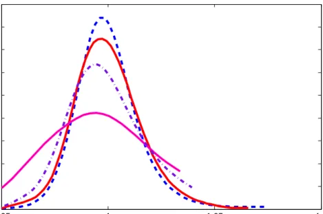
Figure 1: Examples of inter-temporal pricing kernels (as functions of moneyness) with fixed maturity 0.00833 (3 days) in years respectively on 17-Jan-2006 (blue), 18-Apr-2006 (red), 16-May-2006 (magenta), 13-June-2006 (black), see Grith, H¨ardle and Park (2009).
The above mentioned theory allows us to relate prices processes of assets traded in the market to risk preference of investors. This amounts to fit a flexible model to make inference on the dynamics of EPKs over time in different markets. A well-known but restrictive approach is to assume the underlying following a Geometric Brownian Motion. In this setting, risk neutral densities and historical densities are log normal distributions with different drifts, and the pricing kernel has the form of a derivative of a power util-ity. Thus it is decreasing in return and implies overall-risk averse behavior. However,
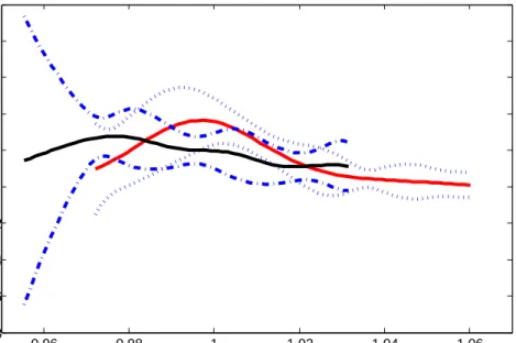
across different markets, one observes quite often a non-decreasing pattern for EPKs, a phenomenon is called the EPK paradox, see Chabi-Yo, Garcia and Renault (2008). Two plots of pricing kernels are shown in Figure 1 and Figure 2. Figure 1 depicts inter-temporal pricing kernels with fixed maturity, while Figure 2 depicts pricing kernels with two different maturities and their confidence bands. The figures are shown on a returns scale. The curves present a bump in the middle and a switch from convexity to concavity in all cases. Especially, this shows that very unlikely the bands contain a monotone decreasing curve. 0.96 0.98 1 1.02 1.04 1.06 −8 −6 −4 −2 0 2 4 6 8 10
Figure 2: Examples of inter-temporal pricing kernels with various maturities in years: 0.02222 (8 days, red) 0.1 (36 days, black) on 12-Jan-2006 and their confidence bands.
In order to study the EPK paradox, the time varying coverage probability of a uniform confidence band gives us reliable information. At a fixed point in time, it helps us to test alternatives for a PK and thus yields insights into time varying risk patterns. A test on monotonicity of the PK has been proposed by Golubev, H¨ardle and Timofeev (2009), the extracted time varying parameter, realized either from a low dimensional model for PK or given the coverage probability, may thus be economically analyzed in connection with exogenous macroeconomic business cycle indicator, e.g. credit spread, yield curve, etc, see also Grith, H¨ardle and Park (2009).
Several econometric studies are concerned with estimating PKs by estimating a risk neu-tral density and historical density separately. See section 2 for details. It is stressed in A¨ıt-Sahalia and Lo (1998) that nonparametric inference from pricing kernels gives unbi-ased insights into the properties of asset markets. The stochastic fluctuation of EPK as measured by the maximum deviation has not been studied yet. However, the asymptotic distribution of the maximum deviation and the uniform confidence band linked to it are very useful for model check.
Uniform confidence bands for smooth curves have first been developed for kernel density estimators by Bickel and Rosenblatt (1973), Extension to regression smoothing can be found in Liero (1982) and H¨ardle (1989). But only recently, the results have been carried
over to derivative smoothing by Claeskens and Van Keilegom (2003). Our theoretical path follows largely their results, but our results are applied to a ratio estimator instead of just a local polynomial estimator. Additionally, we extend their results into the second dimension by including the maturity. Also we have a realistic data situation that relates coverage to economic indicators. In addition we perform the smoothing in an implied volatility space which brings by itself an interesting modification of the results of that paper.
The paper is organized as follows: In Section 2, we describe the theoretical connection between utility functions and pricing kernels. In Section 3, we present a nonparametric framework for the estimation of both the historical and the risk neutral density and derive the asymptotic distribution of the maximum deviation. In Section 4, we simulate the asymptotic behavior of the uniform confidence band and compare it with the bootstrap method. Moreover, we also compare the result with other parametric estimations. In Section 5, we conclude and discuss our results.
2
Empirical Pricing Kernel Estimation
Consider an arbitrary risky financial security with the price process{St}t∈[0,T]. We assume
that {St} is a nonnegative semi-martingale with continuous marginals. In a dynamic
equilibrium model the price of the security at time t is equal to the expected net present value of its future payoffs. The interest rate process r is deterministic. We assume that the market is complete, i.e. there exists one positive r.v. π such that
E[π] = 1, E ST π E[π|St] |St = erτSt.
From the risk neutral valuation principle, for the nonnegative payoff ψ(ST), it holds
Ee−rτψ(ST)π
=Ee−rτψ(ST)E[π|ST]
.
By factorization, we obtain E[π|ST] =Kπ(ST), implying
Ee−rτψ(ST)π = Z +∞ 0 e−rτψ(x)Kπ(x)pST(x)dx,
wherepST(x) is the pdf of the price ST. The last expression justifies the notion ofpricing
kernel used for Kπ(x). Following Ait-Sahalia and Lo (2000) consider the distribution
QST(x) = PQ(ST ≤ x) =
Rx
−∞π(z)pST(z)dz. Its density function qST is commonly called
the risk neutral distributionof ST orstate price density(SPD). This follows by observing
that, for any ψ,
Ee−rτψ(ST)π = Z +∞ 0 e−rτψ(x)qST(x)dx. (1)
This implies thatKπ = qST
pST and both the pdf of the future payoff and the SPD are required
to compute the EPK. Several approaches are available to determine the EPK explicitly. First, we can impose strict parametric restrictions on the dynamics of the asset prices and on the distribution of the future payoff. An example are mixture normal distributions, Jackwerth (2000). In the case of more complex stochastic processes, usually no explicit
solution is available. A possible technique though is to use the Brownian motion setup as prior model. Subsequently the SPD is estimated by minimizing the distance to the prior SPD subject to the constraints characterizing the underlying securities, see Rubinstein (1994) and Jackwerth and Rubinstein (1996). Second, the EPK can be determined from the utility function of the agent. Let the aim the investor be to solve the problem:
max
Wt
{u(Wt) +E
t[βu(WT)]},
where u(·) denotes the utility function, Wt the wealth and β the subjective discount
factor. It can be shown that the stochastic discount factor is proportional to the EPK and is given by e−rτqST(s) pST(s) =β u 0(s) u0(S t) .
This implies that by fixing the utility of the investor we can determine the EPK. In practice, however, usually the opposite procedure is applied. The EPK is statistically estimated and used to determine the utility function or the risk aversion coefficient of the investor.
2.1
EPK and option pricing
Here we consider the SPD qST and the pdf pST separately. For notational convenience
we drop the index and write simply q and p. The latter can easily be estimated either parametrically or nonparametrically from the time series of payoffs. On the contrary, the SPD depends on risk preferences and therefore the past observed stock time series do not contain information. Option prices do reflect preferences and, therefore, can be used to estimate the SPD q. Let C(St, X, τ, r, σ2) denote the European call-option price as a
function of the strike price X, priceSt, maturityτ, interest rate r.
q(ST) =erτ ∂2C ∂K2 K=ST .
In a Black-Scholes (BS) framework, where the underlying asset priceStfollows a geometric
Brownian motion. The European options are priced via:
C(St, X, τ, r, σ2) = StΦ(d1)−XerτΦ(d2),
where d1 and d2 are known functions of σ2, τ, X and St. This implies that both q(ST)
and p(ST) are lognormal distributions:
q(ST) = 1 ST √ 2πσ2τ exp −{log(ST/St)−(r−σ 2/2)τ}2 2σ2τ (2) and p(ST) with µ replacing r in (2).
Beside the modeling bias that is implicit in the BS model, it is also not possible to reflect the implicit volatility smile (surface) as a function of X and τ via (2). The latter may be derived in stochastic volatility models of Heston or Bates type or even more complex parametrizations. In order to study unbiased risk patterns, we need to guarantee models for the pricing kernel that are rich enough to reflect local risk aversion in time and space. This leads naturally to a smoothing approach.
Consider call options with maturity maturity τ. The intraday call options are observed
Yi =Cτ(Xi) +σ(Xi)εi, i= 1, . . . , nq, (3)
whereYi denotes the observed option price andKi the strike price. Yi andXi are assumed
to be i.i.d. in the cross section with Var(Yi|X = Xi) = σ2(Xi). It should be said that
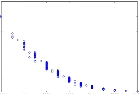
the perceived errors are due to neglected heterogeneity factors, rather than mispricings exploited by arbitrage strategies, see Renault (1997). Figure 3 depicts the call option prices data used to calculate a SPD. The observations are distributed with different vari-ances at discrete grid points of strikes prices. For simplicity of notation, we write C(X)
62000 6400 6600 6800 7000 7200 7400 100 200 300 400 500 600
Figure 3: Plot of call option prices against strike prices 20010117
for Cτ(X). Assuming that C(X) is continuously differentiable of order p = 3, it can be
locally approximated by C(X, X0) = p X j=0 Cj(X)(X0−X)j, (4) where Cj(X) =C(j)(X)/j!, j = 0, . . . , p.
See Cleveland (1979), Fan (1992), Fan (1993), Ruppert and Wand (1994) for more details. Assuming local Gaussian quasi-likelihood model, we arrive at:
Bnq{C(X)}= 1 nq nq X i=1 Khnq(Xi−X)Q{Yi, C(X, Xi)}, (5)
whereKhnq(Xi−X) is a (Gaussian) kernel function with a bandwidth sequencehnq. The
vector of solutions isC(X) ={C0(X), C1(X), . . . , Cp(X)}> is obtained via the
optimiza-tion problem
ˆ
C(X) = arg max
where E is a certain compact set. This is equivalent to solving Anq(X) def = 1 nq nq X i=1 Khq(Xi−X) ∂Q{Yi, C(X, Xi)} ∂C Xi = 0, (7) with Xi def
= (1, Xi − X,(Xi − X)2,(Xi − X)3)>. We are concerned with 2! ˆC2(x) =
∂2C(X)
∂X2
X=x, which is shown by Breeden and Litzenberger (1978) to be proportional to
q(x).
In practice we assume a Gaussian quasi-likelihood function with Q{Y, C(X)}= 1/2{Y −
C(X)}2/σ2(X), which is equivalent to local least squares smoothing. Additionally note
that we assume the parameter C(.) and σ(.) to be orthogonal to each other. Thus we can estimate them separately as in a single parameter case. Let Anq,j denote the jth
component of the vector equationAnq. This component corresponds to thej-th derivative
of the option price evaluated atX. The following lemma states the results on the existence of the solution and its consistency.
Lemma 1 Under conditions (A1) − (A5), there exists a sequence of solutions to the equations Anq(x) = 0 such that sup x∈E |qˆ(x)−q(x)|=O h−nq2{lognq/(nqhnq)} 1/2 +h2nq a.s.
The density of the returns can be estimated separately from the SPD using historical prices S1, . . . , Snp of the underlying asset. The nonparametric kernel estimator of pST is
given by ˆ p(x) =n−p1 np X j=1 Khnp(x−Sj),
wherehnp is the bandwidth of the kernelLwhich not necessarily coincides with the kernel
for q. Under assumption (A5), we know that sup
x∈E
|pˆ(x)−p(x)|=O{(nphnp/lognp)
−1/2+h2
np}. (8)
The estimator of the EPK is then given by the ratio of the estimated SPD and the risk-neutral density, i.e. ˆK(x) = ˆq(x)/pˆ(x). The next lemma provides the linearization of the ratio, which is important for further statements about the uniform confidence band of the EPK.
Lemma 2 Under conditions (A1)-(A5) it holds
sup x∈E |Kˆ(x)− K(x)| = sup x∈E ˆ q(x)−q(x) p(x) − ˆ p(x)−p(x) p(x) · q(x) p(x) − {qˆ(x)−q(x)}{pˆ(x)−p(x)} p2(x) +O[max{(nphnp/lognp)−1/2+h2n p, h −2 nq{nqhnq/lognq} −1/2 +h2nq}]. (9)
This lemma implies that the stochastic deviation of Kb can be linearized into a stochastic
part containing the estimator of the SPD and a deterministic part containingE[ˆp(x)]. The uniform convergence can be proved by dealing separately with the two parts. The conver-gence of the deterministic part is shown by imposing mild smoothness conditions, while the convergence of the stochastic part is proved by following the approach of Claeskens and Van Keilegom (2003). Theorem 1 formalizes this uniform convergence of the EPK.
Theorem 1 Under conditions (A1)−(A5) and for all x∈E, it holds
sup x∈E |Kˆ(x)− K(x)|=O[max{(nphnp/lognp) −1/2+h2 np, h −2 nq{nqhnq/lognq} −1/2+h2 nq}] a.s.
The proof is given in the appendix.
3
Confidence intervals and confidence bands
Confidence intervals characterize the local precision of the EPK for a given fixed value of the payoff. This allows to test EPKs at each particular return, but does not allow conclusions about the global shape. The confidence bands, however, characterize the whole EPK curve and offer therefore the possibility to test for shape characteristics. In particular, it is a way to check the persistence of the bump as observed. Give a certain shape rejection, one may verify the restriction imposed by the power utility and obtain insights about the risk aversion of the agents. In addition, the confidence bands can be used to measure the global variability of the EPK. Also, the proportion of BS fitting covered in nonparametric bands can be used as a measure of global risk aversion.
A confidence interval for the EPK at a fixed valuex requires the asymptotic distribution of ˆp(x) and ˆq(x). Hereafter, we useLto denote the convergence in law. Under (A1)-(A5):
q nphnp{pˆ(x)−p(x)} L −→N{0, p(x) Z K2(u)du} and q nqh5nq{qˆ(x)−q(x)} L −→, N{0, σq2(x)},
where σq2 = [B(x)−1N−1T N−1](3,3), with B(x) equal to the product of the density fX(x)
of the strike price and the local Fisher information matrixI{C(x)}. The matricesN and
T are given by N def= [R
ui+jK(u)du] i,j and T def = [R ui+jK2(u)du] i,j with i, j = 0, . . . ,3.
This implies the asymptotic normality of the estimated EPK at a fixed payoff x. More precisely
q
nqh5q{Kˆ(x)− K(x)}
L
−→N{0, σq2(x)/p2(x)}.
Let the time pointt and the time to maturityτ be fixed. The respective EPK is denoted by ˆK(x)). The variance of ˆK= ˆK(x) is given by
Var{Kˆ(x)} ≈ {p(x)}−2B−1(x)N−1T N−1. (10)
LetDn(x) be the standardized process:
Dn(x)
def
= n1q/2hnq
5/2{Kˆ(x)− K(x)}/[Var{Kˆ(x)}]1/2.
Theorem 2 Under assumptions A(1)-(A5) it follows P (−2 loghnq) 1/2 sup x∈E |Dˆn(x)| −cnt < z −→exp{−2 exp(−z)}, where cnt = (−2 loghnq) 1/2+ (−2 logh nq) −1/2{x α+ log(R/2π)}.
The (1−α)100% confidence band for the pricing kernel Kis thus: [f : sup
x∈E
{|Kˆ(x)−f(x)|/Varc( ˆK)1/2} ≤Lα],
where Lα = 2!(nqh5nq)
−1/2c
nt, xα=−log{−1/2 log(1−α)} and
R = (N−1M N−1) 3,3/(N−1T N−1)3,3 with M = [ R ui+j{K0 hnq(u)} 2du− 1 2{i(i−1) +j(j− 1)}R ui+j−2K2 hnq(u)du]i,j=0,...,3.
For the implementation with real data we need a consistent estimator ofVar( ˆK). For fixed
τ, we rely on the delta method and use the empirical sandwich estimator, see Carroll, Ruppert and Welsh (1998). The latter method provides the variance estimator for the parameters obtained from estimating equations given by (7).
For the data points (Xit, Yit), i= 1,· · · , n; t =t+ 1,· · · , t+τ, we have
c Var{Kˆ(x)}={pˆ(x)}−2V(x)−1U(x)V(x)−1, where V(x) = 1 nqτ nq X i=1 t+τ X j=t+1 Kh2nq(Xij −x) ∂ ∂CQ{Yij; ˆC(x, Xij)} 2 (Hn−q1Xij)(Hn−q1Xij) > , (11) U(x) = 1 nqτ nq X i=1 t+τ X j=t+1 Kh2nq(Xij −x) ∂2 ∂2CQ{Yij; ˆC(x, Xij)} (Hn−q1Xij)(Hn−q1Xij) > , (12)
whereXij = (1,· · · ,(Xij−x)3)> andhnq = diag{1, . . . , h
3
nq}. The estimator is consistent
in our setup as motivated in Appendix A.2 of Carroll et al. (1998).
3.1
The sheet in maturity dimension
Note that the asymptotic behavior of ˆq(x)−q(x) if correctly standardized does not depend onτ. If we estimate the variance function of ˆKτ(x) in time, we can extend the confidence
band as a sheet to the τ dimension. Let x be the set of maturities of interest. The joint confidence sheet over payoff and maturity is given by
[f : sup
x∈E,τ∈x
{|Kˆτ(x)−f(x)|/ Var( ˆKτ)1/2} ≤Lα].
In the BS setup we can actually provide an explicit link between the EPKs for different maturities. For fixed maturityτ, interest rater we obtain from the normal form of pand
q: Kτ(x) = exp{ (µ−r)(µ+r−σ2)τ 2σ2 }( x St )(µ−r)/σ2.
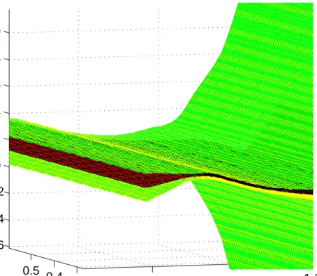
1 1.05 1.1 0.3 0.4 0.5 −6 −4 −2 0 2 4 6 8 10
Figure 4: Examples of sheet for pricing kernels in 060228
This implies
Kτ1(x)/Kτ2(x) = exp{(µ−r)(µ+r−σ 2)(τ
1−τ2)/(2σ2)}
= [exp{τ1−τ2}]c(µ,r,σ)=g(τ1−τ2),
for any fixed τ1 and τ2, i.e. the log difference of the PKs is proportional to the difference
of the maturities. In fact, this gives us some insight into the evolution of the sheet over maturities. More precisely, for known characteristics of the band for fixed τ1, the
confidence band for τ2 is given by
[f : ˆg(τ1−τ2){−LαVarc( ˆKτ1) + ˆKτ1(x)} ≤f(x)≤ˆg(τ1−τ2){LαVarc( ˆKτ1) + ˆKτ1(x)}] for all x∈E.
3.2
Confidence bands based on smoothing implied volatility
The construction of the EPK estimator can be stabilized by a two-step procedure as in Rookley (1997), Fengler (2010). At the first step, we estimate the implied volatility (IV) function by a local polynomial regression. At the second step, we plug the smoothed IV into the BS formula to obtain a semiparametric estimator of the option price. Since the BS model is homogeneous with respect to the asset price and the strike price we smooth the IV using a local polynomial regression in moneyness (Mt). In the absence of dividends,
it is defined at time t asMit=St/Xi. The heteroscedastic model for the IV is given by:
σi =σ(Mit) +
p
where υi are the i.i.d. errors with zero mean and unit variance and η(·) is the volatility
function.
Defining the rescaled call option price by c(Mit) =Ci/St, we obtain from the BS formula
c(Mit) =c{Mit;σ(Mit)}= Φ{d1(Mit)} − e−rτΦ{d 2(Mit)} Mit , where d1(Mit) = log(Mit) + rt+ 12σ(Mit)2 τ σ(Mit) √ τ , d2(Mit) = d1(Mit)−σ(Mit) √ τ .
Combining the result of Breeden and Litzenberger (1978) with the expression for c(Mit)
leads to the SPD q(X) =erτ∂ 2C ∂X2 =e rτS t ∂2c ∂X2 (14) with ∂2c ∂X2 = d2c dM2 M X 2 + 2 dc dM M X2. (15)
As it is shown in the appendix the derivatives in the last expression can be determined explicitly and are functions of V = σ(M), V0 = ∂σ(M)/∂M and V00 = ∂2σ(M)/∂M2. We estimate the latter quantities by the nonparametric local polynomial regression for the IV of the from
σ(Mit) = V(M) +V0(M)(Mit−M) +
1 2V
00
(M)(Mit−M)2.
The respective estimators are denoted by ˆV, ˆV0 and ˆV00. Plugging the results into (14)-(15) we obtain the estimator of SPD in the smoothed IV space. Assuming that the IV process fulfills the the assumptions (A1)-(A5) in the appendix, we conclude that Theorem 2.1 of Claeskens and Van Keilegom (2003) holds also for ˆV, ˆV0 and ˆV00. Note that the convergence rate of ˆV and ˆV0 is lower than of ˆV00. Relying on this fact, we state the asymptotic behavior of ˆq(x)−q(x) in the next theorem.
Theorem 3 Let σ(Mit) satisfy the assumptions (A1)-(A5). Then
ˆ q(x)−q(x) = erτSt M2 X2 h φ{dˆ1(M)} √ τ /2− log(M) +rτ ˆ V(M)2√τ −e−rτφ{dˆ2(M)} −√τ /2−log(M) +rτ ˆ V(M)2√τ i {Vˆ00(M)−V00(M)} +O{Vˆ00(M)−V00(M)}.
Theorem 3 allows us to construct the confidence bands of the SPD estimated semipara-metrically using the confidence bands for the IV. The variance of the estimator is obtained by the delta method in the following way
Var{qˆ(x)−q(x)}= ∂q
∂V00
2
Var{Vˆ00(M)−V00(M)}.
Here it is sufficient to consider only the variance of second derivative of V. The first derivative andV itself can be neglected. The varianceVar{Vˆ00(M)−V00(M)}is estimated using sandwich estimator similarly to (10).
3.3
Bootstrap confidence bands
Hall (1991a) showed that for density estimators, the supremum of{bq(x)−q(x)}converges at the slow rate (lognq)−1 to the Gumbel extreme value distribution. Therefore the
con-fidence band may exhibit poor performance in finite samples. An alternative approach is to use the bootstrap method. Claeskens and Van Keilegom (2003) used smooth bootstrap for the numerical approximation to the critical value. Here we consider the bootstrap technique of the leading term in Lemma 2
sup
x∈E
|qb(x)−q(x)
p(x) |.
We resample data from the smoothed bivariate distribution of (X, Y), the density esti-mator is: ˆ f(x, y) = σˆX nqhnqhnqσˆY nq X i=1 K nXi−x hnq ,(Yi−y)ˆσX hnqσˆY o ,
where ˆσX and ˆσY are the estimated standard deviations of the distributions ofX and Y.
The motivation of using the smooth bootstrap procedure is that a Rosenblatt transfor-mation requires the resampled data (X∗, Y∗) to be continuously distributed.
From the re-sampled data sets, we calculate the bootstrap analogue: sup x∈E |qˆ ∗ (x)−qˆ(x) ˆ p(x) |.
One may argue that this resampling technique does not correctly reflect the bias arising in estimated q, H¨ardle and Marron (1991) use therefore a resampling procedure based on a larger bandwidth g. This refined bias-correcting bootstrap method is not required in our case, since the bandwidth conditions ensure a negligible bias asymptotically.
Correspondingly, we define the one-step estimator for the stochastic deviation by:
h2n q{ ˆ K(x)∗−Kˆ(x)}=−{p(x)}−2{U(x)−1H−1 nqA ∗ nq(x)}3,3
with the variance estimated from the bootstrap sample as:
Var{Kb(x)} ≈ {p(x)}−2B(x)−1N−1M∗N−1. (16)
Lemma 3 Assume conditions (A1)-(A5), a (1−α)100% bootstrap confidence band for the EPK K(x) is:
[f(x) : sup
x∈E
{|Kb(x)−f(x)|V ard(Kb)−1/2} ≤L∗α],
where the bound L∗αj satisfies
P∗[−{U(x)−1Hn−1 qA ∗ nq(x)}3,3/{B(x) −1N−1M∗N−1} 3,3 ≤L∗α] = 1−α.
4
Monte-Carlo study
The practical performance of the above theoretical considerations is investigated via two Monto-Carlo studies. The first simulation aims at evaluating the performance under the BS hypothesis, while the second simulation setup does the same under a realistically calibrated surface. The confidence bands are applied to DAX index options. We first study the confidence bands under a BS null model. Naturally, without volatility smile, both the BS estimator and nonparametric estimator are expected to be covered by the bands. While in the presence of volatility smile, we expect our tests to reject the BS hypothesis in most cases.
4.1
How well is the BS model covered?
In the first setting, we calibrate a BS model on day 20010117 with the interest rate set equal to the short rate r = 0.0481, S0 = 6500, strike prices in the interval [6000,7400].
We refer to A¨ıt-Sahalia and Duarte (2003) on the sources of the noise and use an identical simulation setting, with the noise being uniformly distributed in the interval [0,6]. Fig 5 is a scatter plot of generated observations, the data is clustered in discrete values of the strike price.
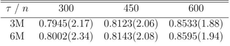
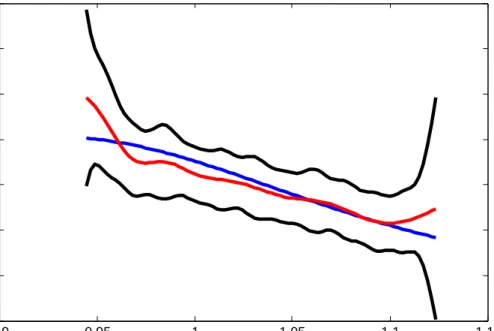
Figure 6 shows a nonparametric estimator for the SPD and a parametric BS estimator. The two estimators roughly coincide except for a small wiggle, thus the bands drawn around the nonparametric curve also fully cover the parametric one. The accuracy is evaluated by calculating the coverage probabilities and average area within the bands, see Table 1 and Table 2. The coverage probabilities is determined via 500 simulations, whenever the hypothesized curve calculated on a grid of 100. The coverage probability approaches its nominal level with the sample size. The bands get narrower with increasing sample sizes. However, the coverage probabilities never reach the nominal level, which may well be attributed to the above mentioned poor convergence of Gaussian maxima to the Gumbel distribution. The area within the bands reflects the stability of the estimation procedure.
Table 1: Coverage probability (area) of the uniform confidence band at 10% with annu-alized volatility = 0.1878 for SPD
τ / n 300 450 600
3M 0.7945(2.17) 0.8123(2.06) 0.8533(1.88) 6M 0.8002(2.34) 0.8143(2.08) 0.8595(1.94)
Table 2: Coverage probability (area) of the uniform confidence band at 5% with annualized volatility = 0.1878 for SPD
τ / n 300 450 600
3M 0.9063(2.402) 0.9144(2.204) 0.9233(1.998) 6M 0.8964(2.438) 0.9056(2.134) 0.9203(2.069)
Historical densities are estimated from simulated stock prices following geometric Brow-nian motion with µ = 0.23. Therefore, a BS EPK estimator could be tested using the
60000 6200 6400 6600 6800 7000 7200 7400 100 200 300 400 500 600 700
Figure 5: Generated noisy BS call option prices against strike prices
above procedure. Due to boundary effects, we concentrate on moneyness (Mt = St/X)
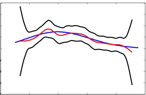
in [0.95,1.1]. Figure 7 displays the nonparametric EPK with confidence band and the BS EPK covered in the band. We observe that the BS EPK is strictly monotonically decreasing. The summary statistics is given in Table 3 and Table 4, due to the additional source of randomness introduced through the estimation of p(x), the coverage probabili-ties are less precise than the corresponding coverage probabiliprobabili-ties for SPD. Nevertheless, the probabilities are getting closer to their nominal values and the bands get narrower when the sample size increases.
Table 3: Coverage probability (area) of the uniform confidence band for the EPK at 5% with volatility(annualized) = 0.1878
M/n 300 450 600
3 0.7820(2.5434) 0.7980(2.4978) 0.8020(2.3876) 6 0.8602(2.4987) 0.8749(2.4307) 0.8900(2.4131)
Table 4: Coverage probability (area) of the uniform confidence band for the EPK at 10% with volatility(annualized) = 0.1878
M/n 300 450 600
3 0.7062(2.4714) 0.7356(2.3410) 0.7620(2.2310) 6 0.7289(2.5020) 0.7740(2.2304) 0.8290(2.3131)
4.2
How well is the band in reality?
Section 4.1 studied the performance of the bands under the BS null, while this section is designed to investigate the performance of the bands when the null hypothesis is violated
0.9 0.95 1 1.05 1.1 1.15 −20 −15 −10 −5 0 5 10 15 20
SPD and its uniform confidence band
Figure 6: Estimation of SPD (red), bands (black) and the BS SPD (blue), with hnq =
0.085, α= 0.05, nq = 300
by a realistic volatility smile observed in the market. For the features of the implied volatility smile we refer to e.g. Fengler (2005). Keeping the parameters identical to the setup of the first study, we generated the data with a smoothed volatility function based on 20010117 withτ = 3M,6M to maturity.
Figure 8 and 9 report the estimators for SPD and EPK. The bands do not cover the BS estimator. Correspondingly, Table 5 and Table 6 show the coverage probabilities, which rapidly decrease when sample sizes are increasing. However, the area within the bands does not change significantly when compared with the results of Section 4.1. We conclude that the confidence bands are useful for detecting the deviation from the BS model.
Table 5: Coverage probability (area) of the uniform confidence band for the EPK at 5%
τ / n 300 450 600
3M 0.5120(2.4320) 0.1784(2.2340) 0.0500(2.0176) 6M 0.5920(2.5304) 0.4100(2.1678) 0.1780(2.0234)
Table 6: Coverage probability (area) of the uniform confidence band for the EPK at 10%
τ / n 300 450 600
3M 0.2580(2.1196) 0.0500(2.0483) 0.0300(2.0132) 6M 0.3746(2.2234) 0.4100(2.1324) 0.1780(2.0030)
0.9 0.95 1 1.05 1.1 1.15 −0.5 0 0.5 1 1.5 2 2.5 3
Figure 7: Estimation of EPK (red), bands (black) and the BS EPK (blue), with hnq =
0.085, α= 0.05, n= 300
5
An illustration with DAX data
5.1
Data
In contrast to previous studies that are mainly based on S&P500 data, we focus on intra-day European options based on the DAX. The source is the European Exchange EUREX and data available by C.A.S.E., RDC SFB 649 (http://sfb649.wiwi.hu-berlin.de) in Berlin. The extracted observations for our analysis cover the period between 1998 and 2008. Fig-ure 10 shows the DAX index. The semiparametric SPD estimates of Rookley (1997) are applied to estimate the EPK. We fix maturity and concentrate on the moneyness dimen-sion. As we cannot find traded options with the same maturity on each day, we consider options with maturity 15 days (10 trading days) across several years. Specifically, we extract a time series of options for every month from Jan 2001 to Dec 2006; this adds up to 63 days.
To make sure that the data correctly represents the market conditions, we use several cleaning criteria. In our sample, we eliminate the observations withτ <1DandIV >0.7. Also, we skip the option quotes violating general no-arbitrage condition i.e. S > C >
max{0, S−Ke−rτ}. Due to the put-call parity, out-of-the-money call options and
in-the-money puts are used to compute the smoothed volatility surface. The median is used to compute the risk neutral density. We use a window of 500 returns for nonparametric kernel density estimators of HD.
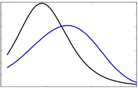
Figure 11 describes the relative position of the HD and SPD on a specific day, the EPK peak is apparently created through the different probability mass contributions at different moneyness states.
0.9 0.95 1 1.05 1.1 1.15 −6 −4 −2 0 2 4 6
SPD and its uniform confidence band
Figure 8: Plot of confidence bands (black), estimated value (red), the BS (blue) SPD with simulated volatility smile, np = 2000, nq = 300, hnq = 0.06, hnp = 0.0106, α= 0.05.
Figure 9: Plot of confidence bands (black), estimated value (red), the BS (blue) EPK with simulated volatility smile np = 2000, nq = 300, hnq = 0.06, hnp = 0.0106, α = 0.05.
1999 2000 2001 2002 2003 2004 2005 2006 2007 2008 2000 3000 4000 5000 6000 7000 8000 9000
Figure 10: Plot of DAX Index
0.950 1 1.05 1.1 2 4 6 8 10 12 14
Figure 11: Plot of estimated state price density (Rookley’s method,hnq = 0.0600) (black)
5.2
Estimation of DAX EPK and its uniform confidence band
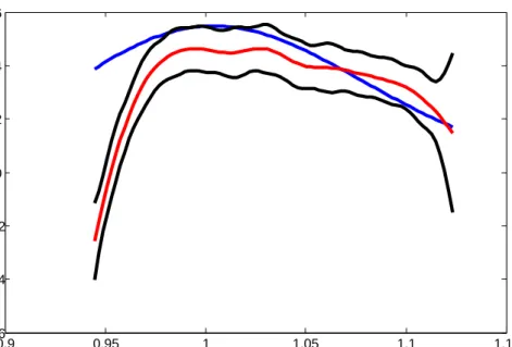
0.95 1 1.05 1.1 −6 −4 −2 0 2 4 6 8 10 12 (a) 060214,τ = 13D 0.95 1 1.05 1.1 −1 0 1 2 3 4 5 (b) 060301,τ= 27D 0.95 1 1.05 1.1 −2 −1 0 1 2 3 4 5 6 7 8 (c) 060305,τ = 20D 0.95 1 1.05 1.1 −1 0 1 2 3 4 5 6 (d) 060417,τ= 27D 0.95 1 1.05 1.1 −6 −4 −2 0 2 4 6 (e) 060419,τ= 13D 0.95 1 1.05 1.1 −2 −1 0 1 2 3 4 5 (f) 060512,τ= 20DFigure 12: BS EPK (black), Rookley EPK (red), Uniform Confidence band (blue) for
α= 0.05
We consider two specifications for the pricing kernels. In the first specification, the BS pricing kernels have a marginal rate of substitution with power utility function:
K(M) = β0M−β1, (17)
where β0 is a scaling factor and β1 determines the slope of pricing kernel. Thus the BS
calibration is realized by linearly regressing the (ordered) log-EPK on log-moneyness. In the second specification, we construct the nonparametric confidence bands as described in Section 3.2,. A sequence of EPKs and corresponding bands are shown in Figure 12. In most of the cases, the BS EPKs are rejected via the confidence bands. The amount of deviation from the hypothesized BS specification though provides us valuable information about how risk hungry investors are. Besides, the area of the bands varies over time, which gives us insights into the variabilities of the prevailing risk patterns. In sum, the bands not
only provide a simple test for hypothesizes EPKs but also help us to study the dynamics risk patterns over time.
2001010 200112 200208 200302 200411 200509 200611 0.1 0.2 0.3 0.4 0.5 0.6 0.7 0.8 0.9 1
Figure 13: Coverage probability and the DAX index ( rescale to [0,1])
200101−3 200112 200208 200302 200411 200509 200611 −2 −1 0 1 2 3
Figure 14: First difference of coverage probability and the DAX index return (standard-ized)
5.3
Linking economic conditions to EPK dynamics
We use two different indicators for the deviation from the simple BS model. As an approximation to the coverage probability, we calculate the proportion of grid points of the band which covers the BS EPK. As a second measure, we introduce the average width of the confidence band over the moneyness interval [0.95,1.1] as a proxy for the area
between the confidence bands. This provides us with a measure of variability, see also Theorem 2.
The first risk pattern time series are given in Figure 13, where we display the DAX index (scaled to [0,1]) together with the coverage probability. We discover that the coverage probability becomes less volatile when the DAX index level is high. Figure 14 shows the differenced time series. From a simple correlation analysis, we argue that the change in coverage probability and DAX return (with a lag of 3M) are highly negatively correlated (correlation−0.3543) when the DAX index goes down (200101-200302). On the contrary, in the period when the DAX goes up, one observes a large positive correlation (0.3151). What does this mean economically? This implies in a period of worsening economic condition, a positive part of the monthly DAX returns induces a greater hunger for risk in a delay horizon of 3 months. Positive returns have just the opposite effects. With boosting and bullish markets, the positive correlation indicates a 3-month horizon of decreasing risk aversion.
As far as the average width of the bands is concerned, we may conclude from Figure 15 and Figure 16 that in periods of clearly bullish or bearish momentum, the volatility of the width of the confidence band is higher. This may be caused by the uncertainty of the market participants about the long-term persistence of the trend. The lag effect on risk hunger is also detectable for this constructed indicator. Over the whole observation interval, the correlation between the monthly DAX return and the change in the average width is−0.3230 for a 1M lag and −0.2717 for 3M.
2001010 200112 200208 200302 200411 200509 200611 0.2 0.4 0.6 0.8 1
Figure 15: Area between the bands and the DAX index (scaled to [0,1])
6
Conclusions
Pricing Kernels are important elements in understanding investment behavior since they reflect the relative weights given by investors states of nature (Arrow-Debreu securities). Pricing kernels may be deduced in either parametric or nonparametric approaches. Para-metric approaches like a simple BS model are too restrictive to account for the dynamics
200101−4 200112 200208 200302 200411 200509 200611 −3 −2 −1 0 1 2 3 4
Figure 16: First difference of the area between the bands and the DAX index return (standardized)
of the risk patterns, which induces the well-known EPK paradox. Nonparametric ap-proaches allow more flexibility and reduce the modeling bias. Simple tools like uniform confidence bands help us to conduct tests against any parametric assumption of the EPKs i.e. shape inspection. Considering the numerical stability, we smooth the IV surface via the Rookley’s method, to obtain SPD estimator.
We have studied systematically the methodology of constructing the uniform bands for both semiparametric or nonparametric estimators. Based on the confidence bands, we explored two indicators to measure risk aversion over time and connected it with DAX index, one is the coverage probability measuring the proportion of the BS fitting curve covered in bands, while another one is the area indicator measuring the variability of the estimator. We have found out that there are strong correlations between DAX index and our indicators with lag effects. The smooth bootstrap is studied without a significant improvement in finite sample performance. One interesting further extension would be employing robust smoothers to improve the bootstrap performance.
7
Appendix
Assumptions:
(A1) hnq → 0 in such a way that {lognq/(nqhnq)}
1/2h3
nq → 0, and the optimal
band-width, to guarantee undersmoothing, is of order O{(lognqnq)1/4[(p−j)/2]+3+2j+α}, where
j = 0,1,2,3, andα >0.
(A2) The kernel function K ∈C(1)[−1,1] and takes value 0 on the boundary.
(A3) For the likelihood function Q ∈ C(1)(E) it holds that inf
x∈EQ(x) > 0. C(x) ∈
and is continuous in C for every y. The Fisher information I(C(x)) has a continuous derivative and infx∈EI{C(x)}>0.
(A4) There exists a neighborhood N(C(x)) such that max k=1,2supx∈E || sup C∈N{C(x)} ∂k ∂CkQ(y;C)||λ <∞
for some λ∈(2,∞]. Furthermore sup x∈E E[ sup C∈N(C(x)) | ∂ 3 ∂C3Q(y;C)|]<∞.
(A5) The density of underlyingp(x) is three times continuously differentiable. (A6) Let anp = (nphnp/lognp)
−1/2+h2 np from (8) and bnq =h −2 nq(nqhnq/lognq) −1/2+h2 nq
from Lemma 1. We assume that nq/np =O(1) andanp/bnq =O(1).
7.1
Proof of Lemma
1
We follow the approach of Zhao (1994) also deployed by Claeskens and Van Keilegom (2003). Consider the disturbed coefficients of the local polynomial
Cε(x, X0) = p X j=0 {Cj(x) +εnqj}(X0−x) j,
where εnqj are positive-valued sequences for j = 0, . . . , p+ 1. This leads to the modified
system of equations Anqj,ε(x) = 1 nq nq X i=1 Khnq(Xi−x) ∂Q{Yi, Cε(x, Xi)} ∂C (Xi−x) j.
Similarly to Lemma 2.2 of H¨ardle, Janssen and Serfling (1988) and using assumptions (A1)-(A4), we obtain sup x∈E sup C∈N{C(x)} s nqhnq lognq 1 nqhnq nq X i=1 Khnq(Xi−x) ∂Q{Yi, C(x, Xi)} ∂C (Xi−x)j hjnq −E 1 nqhnq nq X i=1 Khnq(Xi−x) ∂Q{Yi, C(x, Xi)} ∂C (Xi−x)j hjnq =O(1) (a.s.).
This implies that supx∈E|Anqj,ε(x)−EAnqj,ε(x)|=O[h
j
nq{lognq/(nqhnq)}
1/2] =`
nqj (a.s.).
Particularly this implies, that (a.s.) |Anqj,ε(x)−EAnqj,ε(x)| ≤ `nqj for appropriate εnq.
Consider the first order Taylor expansion of∂Q{Yi, Cε(x, Xi)}/∂C around the true values
of the parameters Cj(x) of the polynomial regression.
∂Q{Y, Cε(u, X)} ∂C ≈E h∂Q{Y, C(X)} ∂C i X=u +Eh∂ 2Q{Y, C(X)} ∂C2 i X=u · {Cε(u, X)−C(u)}.
Noting that Eh∂Q{Y,C∂C(X)}i = 0 we obtain E{Anqj,ε(x)} = −E 1 nq nq X i=1 Khnq(Xi−x)(Xi−x) jEh− ∂2Q{Yi, C(X)} ∂C2 i X=u ×{C(u, Xi)−C(u) + p X j∗=0 εnqj∗(Xi−u) j∗}.
Note that sup|u−x|≤hnq
Pp
j∗=0(u− x)j ∗R
uj∗Khnq(u)du = O(1). We decompose the
ex-pectation into two parts, one containing C(u, Xi)−C(u) and the second one containing
Pp j∗=0εnqj∗(Xi−u) j∗}. Let ˜p= 2([p/2] + 1) and ωj(hnq) def = h2[(nqp−j)/2]+1 Z up˜+jKhnq(u)du·sup x∈E Cp˜(x) =O(hn2{q[(p−j)/2]+1}).
The first part is bounded above by M ωj(hnq) for some constant M, while the second
part is bounded by 2`nqj. Choosing εnqj = O(max[2ωj(hnq),4`nqj/M]) we obtain that E[Anqj,ε(x)] ≤ −
1
2M εnqj. Similarly we can show that E[Anqj,−ε(x)] ≥
1 2M εnqj. This implies that Anqj,ε(x)≤ `nqj − 1 2M εnqj <0 and Anqj,−ε(x)≥ −`nqj + 1 2M εnqj >0. Thus
there exists a sequence of estimators ˆCj(x) such that supx∈E|Cˆj(x)−C(x)| ≤ εnqj. The
choice of εnqj implies forj = 2
sup x∈E |qˆ(x)−q(x)|=O[hn−q2{lognq/(nqhnq)} 1/2 +h2nq] (a.s.)
7.2
Proof of Lemma 2
Recall from Lemma 1 and (8) that sup x∈E |pˆ(x)−p(x)|=O{{lognq/(nqhnq)} 1/2+h2 np}=O(anp), sup x∈E |qˆ(x)−q(x)|=O[h−n2 q{lognq/(nqhnq)} 1/2+h2 nq] =O(bnq).
To determine the order of the EPK we linearize the ratio q(x)/p(x). ˆ K(x)− K(x) = qˆ(x) ˆ p(x)− q(x) p(x) = ˆ q(x)p(x)−pˆ(x)q(x) p2(x) · 1 1 + pˆ(xp)(−xp)(x).
We decompose the first factor as ˆq(x)p(x)−pˆ(x)q(x) = {qˆ(x) −q(x)}p(x)− {pˆ(x)−
p(x)}q(x), while for the second factor we use the first order Taylor expansion. Putting together we obtain sup x∈E |Kˆ(x)− K(x)| = sup x∈E |qˆ(x)−q(x) p(x) − ˆ p(x)−p(x) p(x) · q(x) p(x) −{qˆ(x)−q(x)}{pˆ(x)−p(x)} p2(x) + {pˆ(x)−p(x)}2 p2(x) · q(x) p(x)|. The first two elements are of orderO(bnq) andO(anp) respectively, while the last element
is of order O(anp). Summarizing we conclude that sup
x∈E
7.3
Proof of Theorem 2
The basic idea of the proof is to approximate the process
Dnq(x) =n 1/2 q h 5/2 nq {Kˆ(x)− K(x)}/[Varc{Kˆ(x)}] 1/2
by a process with a non-stochastic variance term, which is further approximated by a process that can be treated with the tools of Claeskens and Van Keilegom (2003). Here we drop for the simplicity of notation the indices in nq and hnq. As first approximation
we define
D(1)n (x)def= n1/2h5/2{Kˆ(x)− K(x)}/{VK(x)}1/2,
where VK(x) =Var{Kˆ(x)} is given in equation (10). Lemma 2 ensures that the approxi-mation by
n1/2h5/2{qˆ(x)−q(x)}/{p(x)VK(x)1/2} (18) is uniformly of order Op{(logn)−1/2}. The process in equation (18) can be approximated as in Claeskens and Van Keilegom (2003) by
2! exp(rτ)h2fX(x)−1/2VK(x)−1/2I{C(x)}−1/2 3 X i=0 fX(x)−1/2I{C(x)}−1/2{N−1}3,i+1An,i(x) (19) For the definition of the local Fisher information,I{C(x)}, the matrixN and the process
Ani(x), we refer to Section 3 and Section 7. Define
Yni(x)
def
= (nh)1/2h−i[I{C(x)}fX(x)]−1/2Ani(x).
Then equation (19) can be written as
Fn(x) def = 2! exp(rτ)h2{fX(x)}−1/2VK(x)−1/2I{C(x)}−1/2 3 X i=0 hi{N−1}3,i+1Yni(x)
Please note that N is not a function of x as Claeskens and Van Keilegom (2003) erro-neously write. Following their line of thoughts, we replace Yni(x) (uniformly) by
Yni0(x) = h1/2 Z Kh(z−x) z−x h dz.
In order to apply Corollary A1 of Bickel and Rosenblatt (1973), denote the covariance function of the Gaussian process Fnq(x) by r(x), and note that
r(x) =Cov(Ynj0 (x), Ynj0 (0)) =C1−C2|x|2+O(|x|2)
for x ∈ E, where C1 and C2 are constants. Since the regularity conditions are satisfied,
the result follows.
Finally, we have to show that supx∈E|Varc{Kˆ(x)} −Var{Kˆ(x)}|=Op(1).
sup x∈E |Varc{Kˆ(x)} −Var{Kˆ(x)}| = sup x∈E |Varc nqˆ(x)−q(x) p(x) o −Varnqˆ(x)−q(x) p(x) o |+Op{(nh)−(1/2+α)(logn)1+α},
where 0< α <1.
According to Corollary 2.1 in Claeskens and Van Keilegom (2003), for j = 3, k= 3, sup
x∈E
|Varc{qˆ(x)} −Var{qˆ(x)}|=Op{(nhlogn)−1/2}.
This implies
sup
x∈E
|Varc{Kˆ(x)} −Var{Kˆ(x)}|=Op(1).
7.4
Expressions for the semiparametric estimator of SPD
Taking the derivatives of c(Mit) with respect to moneyness (M) and noting that both
d1(Mit) and d2(Mit) depend on Mit we obtain
dc dM = ϕ(d1) dd1 dM −e −rτϕ(d2) M dd2 dM +e −rτΦ(d2) M2 , d2c dM2 = ϕ(d1) nd2d1 dM2 −d1 dd1 dM 2 o −e −rτϕ(d 2) M nd2d2 dM2 − 2 M dd2 dM −d2 dd2 dM 2 o − 2e −rτΦ(d 2) M3
Computing the first and second order differentials for d1 and d2 using the notation V =
σ(M), V0 =∂σ(M)/∂M and V00 =∂2σ(M)/∂M2, we obtain dd1 dM = 1 M V√τ + n − log(M) +rτ V2√τ + √ τ /2 o V0, dd2 dM = 1 M V√τ + n − log(M) +rτ V2√τ − √ τ /2oV0, d2d1 dM2 = − 1 M V√τ n 1 M + V0 V o +V00n √ τ 2 − log(M) +rτ V2√τ o +V0n2V0log(M) +rτ V3√τ − 1 M V2√τ o , d2d2 dM2 = − 1 M V√τ n 1 M + V0 V o +V00n− √ τ 2 − log(M) +rτ V2√τ o +V0 n 2V0log(M) +rτ V3√τ − 1 M V2√τ o ,
References
A¨ıt-Sahalia, Y. and Duarte, J. (2003). Nonparametric option pricing under shape restric-tions, Journal of Econometrics 116: 9–47.
A¨ıt-Sahalia, Y. and Lo, A. W. (1998). Nonparametric estimation of state-price densities implicit in financial asset prices, The Journal of Finance 53: 499–547.
A¨ıt-Sahalia, Y. and Lo, A. W. (2000). Nonparametric risk management and implied risk aversion, Journal of Econometrics 94: 9–51.
Bickel, P. J. and Rosenblatt, M. (1973). On some global measures of the deviations of density function estimates, The Annals of Statistics 1: 1071–1095.
Breeden, D. and Litzenberger, R. (1978). Prices of state-contingent claims implicit in options prices, The Journal of Business 51: 621–651.
Brown, D. P. and Jackwerth, J. C. (2004). The pricing kernel puzzle: Reconciling index option data and economic theory,Manuscript .
Carroll, R., Ruppert, D. and Welsh, A. (1998). Local estimating equations, Journal of American Statistics Association 93: 214–227.
Chabi-Yo, Y., Garcia, R. and Renault, E. (2008). State dependence can explain the risk aversion puzzle,Review of Financial Studies 21: 973–1011.
Claeskens, G. and Van Keilegom, I. (2003). Bootstrap confidence bands for regression curves and their derivatives, The Annals of Statistics 31: 1852–1884.
Cleveland, W. (1979). Robust locally weighted regression and smoothing scatterplots,
Journal of American Statistical Association 74: 829–836. Cochrane, J. H. (2001). Asset pricing, Princeton University Press.
Fan, J. (1992). Design-adaptive nonparametric regression,Journal of American Statistical Association 87: 998–1004.
Fan, J. (1993). Local linear regression smoothers and their minimax efficiencies, The Annals of Statistics 21: 196–216.
Fengler, M. (2005). Semiparametric modeling of implied volatility, Springer.
Fengler, M. (2010). Option data and modeling of implied volatility,Handbook of Compu-tational Finance, Duan, Gentle, H¨ardle, eds. Springer Verlag .
Golubev, Y., H¨ardle, W. and Timofeev, R. (2009). Testing monotonicity of pricing kernels,
Journal of Applied Econometrics, invited resubmission, 01.12.2009 .
Grith, M., H¨ardle, W. and Park, J. (2009). Shape invariant modelling pricing kernels and risk aversion, Journal of Financial Econometrics, submitted, 01.05.2009.
Hall, P. (1991a). Edgeworth expansions for nonparametric density estimators, with appli-cations, Vol. 22, New York: Academic Press.
H¨ardle, W. (1989). Asymptotic maximal deviation of m-smoothers,Journal of Multivari-ate Analysis 29: 163–179.
H¨ardle, W., Janssen, P. and Serfling, R. (1988). Strong uniform consistency rates for estimators of conditional functionals, Annals of Statistics 16: 1428–1449.
H¨ardle, W. and Marron, J. (1991). Bootstrap simultaneous error bars for nonparametric regression, Annals of Statistics 19: 778–796.
Jackwerth, J. (2000). Recovering risk aversion from option prices and realized returns,
Review of Financial Studies 13: 433–451.
Jackwerth, J. and Rubinstein, M. (1996). Recovering probability distributions from option prices, Journal of Finance 51: 1611–1631.
Kahneman, D. and Tversky, A. (1979). Prospect theory: an analysis of decision under risk, Econometrica 47: 263–291.
Liero, H. (1982). On the maximal deviation of the kernel regression function estimate,
Mathematische Operationsforschung und Statistik, Serie Statistics13: 171–182. Renault, E. (1997). Econometric models of option pricing errors, in D. M. Kreps and
K. F.Wallis (eds), Proceedings the Seventh World Congress of the Econometric Society, Econometric Society Monographs, London: Cambridge University Press, pp. 223–278.
Rookley, C. (1997). Fully exploiting the information content of intra day option quotes: Applications in option pricing and risk management,Manuscript .
Rosenberg, J. and Engle, R. F. (2002). Empirical pricing kernels, Journal of Financial Economics 64: 341–372.
Rubinstein, M. (1994). Implied binomial trees, Journal of Finance 49: 771–818.
Ruppert, D. and Wand, M. (1994). Multivariate locally weighted least squares regression,
The Annals of Statistics 22: 1346–1370.
Zhao, P.-L. (1994). Asymptotics of kernal estimators based on local maximum likelihood,
SFB 649 Discussion Paper Series 2010
For a complete list of Discussion Papers published by the SFB 649, please visit http://sfb649.wiwi.hu-berlin.de.
001 "Volatility Investing with Variance Swaps" by Wolfgang Karl Härdle and Elena Silyakova, January 2010.
002 "Partial Linear Quantile Regression and Bootstrap Confidence Bands" by Wolfgang Karl Härdle, Ya’acov Ritov and Song Song, January 2010. 003 "Uniform confidence bands for pricing kernels" by Wolfgang Karl Härdle,