Mining Clinical Data
Argyris Kalogeratos, V. Chasanis, G. Rakocevic, A. Likas, Z. Babovic, and M. Novakovic
1.1
Data Mining Methodology
The prerequisite of any machine learning or data mining application is to have a clear target variable that the system will try to learn [27]. In a supervised setting, we also need to know the value of this target variable for a set of training examples (i.e., patient records). In the case study presented in this chapter, the value of the considered target variable that can be used for training is the ground truth character-izations of the coronary artery disease severity or, as a different scenario, the progression of the patients. We either set as target variable the disease severity, or disease progression, and then we consider a two-class problem in which we aim to discriminate a group of patients that are characterized as “severely diseased” or “severely progressed,” from a second group containing “mildly diseased” or “mildly progressed” patients, respectively. This latter mild/severe characterization is the actual value of the target variable for each patient.
In many cases, neither the target variable nor its ground truth characterization is strictly specified by medical experts, which is a fact that introduces high complexity
A. Kalogeratos (*) • V. Chasanis • A. Likas
Department of Computer Science, University of Ioannina, GR-45110 Ioannina, Greece e-mail:[email protected];[email protected]
G. Rakocevic
Mathematical Institute, Serbian Academy of Sciences and Arts, Belgrade 11000, Serbia Z. Babovic • M. Novakovic
Innovation Center of the School of Electrical Engineering, University of Belgrade, Belgrade 11000, Serbia
G. Rakocevic et al. (eds.),Computational Medicine in Data Mining and Modeling, DOI 10.1007/978-1-4614-8785-2_1,©Springer Science+Business Media New York 2013
and difficulty to the data mining process. The general data mining methodology we applied is a procedure divided into six stages:
Stage 1:Data mining problem specification
• Specify the objective of the analysis (the target variable).
• Define the ground truth for each training patient example (the specific value of the target variable for each patient).
Stage 2:Data preparation, where some preprocessing of the raw data takes place
• Deal with data inconsistencies, different feature types (numeric and nominal), and missing values.
Stage 4:Data subset selection
• Selection of a feature subset and/or a subgroup of patient records
Stage 5:Training of classifiers
• Build proper classifiers using the selected data subset.
Stage 6:Validate the resulting models
• Using techniques such as v-fold cross-validation. • Compare the performance of different classifiers. • Evaluate the overall quality of the results.
• Understand whether the specification of the data mining problem and/or the definition of the ground truth values are appropriate in terms of what can be extracted as knowledge from the available data.
A popular methodology to solve these classification problems is to use a decision tree (DT) [28]. DTs are popular tools for classification that are relatively fast to both train and make predictions, while they also have several other additional advantages [10]. First, they naturally handle missing data; when a decision is made on a missing value, both subbranches are traversed and a prediction is made using a weighted vote. Second, they naturally handle nominal attributes. For instance, a number of splits can be made equal to the number of the different nominal values. Alternatively, a binary split can be made by grouping the nominal values into subsets. Most important of all, a DT is an interpretable model that represents a set of rules. This is a very desirable property when applying classifica-tion models to medical problems since medical experts can assess the quality of the rules that the DTs provide.
There are several algorithms to train DT models, among the most popular of them are ID3 and its extension C4.5 [2]. The main idea of these algorithms is to start building a tree from its root, and at each tree node, a split of the data in two subsets is determined using the attribute that will result in the minimum entropy (maximum information gain).
DTs are mainly used herein because they are interpretable models and have achieved good classification accuracy in many of the considered problems.
However, other state-of-the-art methods such as the support vector machine (SVM) [3] may provide better accuracy at the cost of not being interpretable. Another powerful algorithm that builds non-interpretable models is the random forest (RF) [18]. An RF consists of a set of random DTs, each of them trained using a small random subset of features. The final decision for a data instance is taken using strategies such as weighted voting on the prediction of the individual random DTs. This also implied that a decision can be made using voting on contradicting rules and explains why these models are not interpretable. In order to assess the quality of the DT models that we build, we compare the classification performance of DTs to other non-interpretable classifiers such as the abovementioned SVM and RF.
Another property of DTs is that they automatically provide a measure of the significance of the features since the most significant features are used near the root of the DT. However, other feature selection methods can also be used to identify which features are significant for the classification tasks that we study [7]. Most feature selection methods search over subsets of the available features to find the subset that maximizes some criterion [4]. Common criteria measure the correlation between features and the target category, such as the information gain (IG) or chi-squared measures. Among the state-of-the-art feature selection techniques are the RFE-SVM [6], mRMR [22], and MDR [13] techniques. They differ to the previous approaches in that they do not use single-feature evaluation criteria. Instead, they try to eliminate redundant features that do not contain much informa-tion. In this way, a feature that is highly correlated with other features is more probable to be eliminated than a feature that may have less IG (as single-feature evaluation measure) comparing to the IG of the first but at the same time carries information that is not highly correlated with other features [11].
1.2
Data Mining Algorithms
In this section we briefly describe the various algorithms used in our study for classifier construction and feature evaluation/selection, as well as the measures we used to assess the generalization performance of the obtained models.
1.2.1
Classification Methods
1.2.1.1 Decision Trees
A decision tree (DT) is a decision support tool that uses a treelike graph represen-tation to illustrate the sequence of decisions made in order to assign an input instance to one of the classes. The internal node of a decision tree corresponds to an attribute test. The branches between the nodes tell us the possible values that these attributes can have in the observed samples, while the terminal (leaf ) nodes provide the final value (classification label) of the dependent variable.
A popular solution is the J48 algorithm for building DTs that has been implemented in the very popular Weka software for DM [2]. It is actually an implementation of the well-known and widely studied C4.5 algorithm for building decision trees [15]. The tree is built in a top-down fashion, and at each step, the algorithm splits a leaf node by identifying the attribute that best discriminates the subset of instances that correspond to that node. A typical criterion that is commonly used to quantify the splitting quality is the information gain. If a node of high-class purity is encountered, then this node is considered as a terminal node and is assigned the label of the major class. Several post-processing pruning operations also take place using a validation in order obtain relatively short trees that are expected to have better generalization.
It is obvious that the great advantage of DTs as classification models is their interpretability, i.e., their ability to provide the sequence of decisions made in order to get the final classification result. Another related advantage is that the learned knowledge is stored in a comprehensible way, since each decision tree can be easily transformed to a set of rules. Those advantages make the decision trees very strong choices for data mining problems especially in the medical domain, where inter-pretability is a critical issue.
1.2.1.2 Random Forests
A random forest (RF) is an ensemble of decision trees (DTs), i.e., it combines the prediction made by multiple DTs, each one generated using a different randomly selected subset of the attributes [18]. The output combination can be done using either simple voting or weighted voting. The RF approach is considered to provide superior results to a single DT and is considered as a very effective classification method competitive to support vector machines. However, its disadvantage com-pared to DTs is that model interpretability is lost since a decision could be made using voting on contradicting rules.
1.2.1.3 Support Vector Machines
The support vector machine classifier (SVM) [6, 16] is a supervised learning technique applicable to both classification and regression. It provides state-of-the-art performance and scales well even with large dimension of the feature vector. More specifically, suppose we are given a training set of l vector with d dimensions, xi∈R
d
, i¼1, . . ., n, and a vector y∈Rlwith yi ∈{1,1} denoting the class
of vector xi. The classical SVM classifier finds an optimal hyperplane which separates data points of two classes in such way that the margin of separation between the two classes is maximized. The margin is the minimal distance from the separating hyperplane to the closest data points of the two classes. Any hyperplane can be written as the set of points x satisfying wTx + b ¼0. The vector w is a normal vector and is perpendicular to the hyperplane. A mapping functionφ(x) is
assumed that maps each training vector to a higher dimensional space, and the corresponding kernel function defined as the inner product K(x,y)¼φT(x) φ(y). Then the SVM classifier is obtained by solving the following primal optimiza-tion problem: min w,b,ξ 1 2w T wþCi Xl i¼1 ξi (1.1) ð1:2Þ whereξiis called slack variable and measures the extent to which the example xi violates the margin condition and C a tuning parameter which controls the balance between training error and the margin. The decision function is thus given from the following equation: sqn X l i¼1 wiK xð i;xÞ þb ! , where K xi;xj ¼ϕT xi ð Þϕ xj (1.3)
A notable characteristic of SVMs is that, after training, usually most of the training instances xihave wi¼0 in the above equation [17]. In other words, they do not contribute to the decision function. Those xifor which wi¼0 are retained in the SVM model and called support vectors (SVs). In our approach we tested the linear SVM (i.e., with linear kernel function K(xi,xj)¼xTi xj) and the SVM with RBF kernel function with no significant performance difference. For this reason we have adopted the linear SVM approach. The optimal value of the parameter C for each classification problem was determined through cross-validation.
1.2.1.4 Naı¨ve Bayes Classifier
The naı¨ve Bayes (NB) [19] is a probabilistic classifier that builds a model p(x|Ck) for the probability density of each class Ck. These models are used to classify a new instance x as follows: First the posterior probability P(Ck|x) is computed for each class Ckusing the Bayes theorem:
P Cð kjxÞ ¼
P xð jCkÞP Cð Þk
P xð Þ (1.4)
where P(x) and P(Ck) represent the a priori probabilities. Then the input x is assigned to the class with maximum P(Ck|x).
In the NB approach, we made the assumption that the attributes xi of x are independent to each other. Thus, P(x|Ck) can be computed as the product of the
one-dimensional densities p(xi|Ck). The assumption of variable independence dras-tically simplifies model generation since the probabilities p(xi|Ck) can be easily estimated, especially in the case of the discrete attributes where they can be computed using histograms (frequencies). The NB approach has been proved successful in the analysis of the genetic data.
1.2.1.5 Bayesian Neural Networks
A new methodology has been recently proposed for training feed-forward neural networks and more specifically the multilayer perceptron (MLP) [29]. This Bayes-ian methodology provides a viable solution to the well-studied problem of estimating the number of hidden units in MLPs. The method is based on treating the MLP as a linear model, whose basis functions are the hidden units. Then, a sparse Bayesian prior is imposed on the weights of the linear model that enforces irrelevant basis functions (equivalently unnecessary hidden units) to be pruned from the model. In order to train the model, an incremental training algorithm is used which, in each iteration, attempts to add a hidden unit to the network and to adjust its parameters assuming a sparse Bayesian learning framework. The method has been tested on several classification problems with performance comparable to SVMs. However, its execution time was much higher compared to SVM.
1.2.1.6 Logistic Regression
Logistic regression (LR) is the most popular traditional method used for statistical modeling [20] of binary response variables, which is the case in most problems of our study. LR has been used extensively in the medical and social sciences. It is actually a linear model in which the logistic function is included in the linear model output to constraint its value in the range from zero to one. In this way, the output can be interpreted as the probability of the input belonging to one of the two classes. Since the underlying model is linear, it is easy to train using various techniques.
1.2.2
Generalization Measures
In order to validate the performance of the classification models and evaluate their generalization ability, a number of typical cross-validation techniques and two performance evaluation measures were used. In this section we will cover two of them: classification accuracy and the kappa statistic.
In k-fold cross-validation [1], we partition the available data into k-folds. Then, iteratively, each of these folds is used as a test set, while the remaining
folds are used to train a classification model, which is evaluated on the test set. The average classifier performance on all test sets provides a unique measure of the classifier’s performance on the discrimination problem. Leave-one-out validation technique is a special case of cross validation, where the test set contains only a single data instance each time that is left out of the training set, i.e., leave-one-out is actual N-fold cross validation where N is the number of data objects.
The accuracy performance evaluation measure is very simple and provides the percentage of correctly classified instances. It must be emphasized that its absolute value is not important in the case of unbalanced problems, i.e., an accuracy of 90 % may not be considered important when the percentage of data instances belonging to the major class is 90 %. For this reason we always report the accuracy gain as well, which is the difference between the accuracy of the classifier and the percent-age of the major class instances.
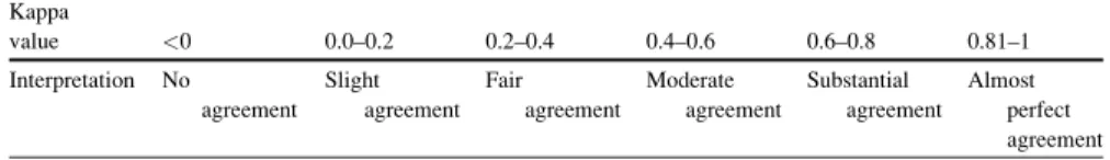
The kappa statistic is another reported evaluation measure calculated as
Kappa¼P Að Þ P Eð Þ
1P Eð Þ (1.5)
where P(A) is the percentage of observed agreement between the predictions and actual values and P(E) the percentage of chance agreement between the predictions and actual values. A typical interpretation of the values of the kappa statistic is provided in Table1.1.
1.2.2.1 Feature Selection and Ranking
A wide variety of feature (or attribute) selection methods have been proposed to identify which features are significant for a classification task [4]. Identification of significant feature subsets is important for two main reasons. First, the complexity of solving the classification problem is reduced, and data quality is improved by ignoring the irrelevant features. Second, in several domains such as medical domain, the identification of discriminative features is actually new knowledge for the problem domain (e.g., discovery of new gene markers using bioinformatics datasets or SNPs in our study using the genetic dataset).
Table 1.1 Interpretation of the kappa statistic value
Kappa value <0 0.0–0.2 0.2–0.4 0.4–0.6 0.6–0.8 0.81–1 Interpretation No agreement Slight agreement Fair agreement Moderate agreement Substantial agreement Almost perfect agreement
1.2.2.2 Single-Feature Evaluation
Simple feature selection methods rank the features using various criteria that measure the discriminative power of each feature when used alone. Typical criteria compute the correlation between the feature and the target category, such as the information gain and chi-squared measure, which we have used in our study.
Information Gain
Information gain (IG) of a feature X with respect to class Y(I(Y;X)) is the reduction in uncertainty about the value of Y when the value of X is known. The uncertainty of a variable X is measured by its entropy H(X), and the uncertainty about the value of Y, when the value of X is known, is given by its conditional entropy H(Y|X). Thus, information gain I(Y;X) can be defined as
I Yð ;XÞ ¼H Yð Þ H Y Xð j Þ (1.6)
For discrete features, the entropies are calculated as
H Yð Þ ¼ X l j¼1 P Y ¼yj log2 P Y¼yj (1.7) H Yð jXÞ ¼ X l j¼1 P X¼xj H Y X ¼xj (1.8)
Alternatively, IG can be calculated as
I Yð ;XÞ ¼H Xð Þ þH Yð Þ H Yð ;XÞ (1.9) For continuous features, discretization is necessary.
Chi-Square
The chi-square (also denoted as chi-squared orχ2) is another popular criterion for feature selection. Features are individually evaluated by measuring their chi-squared statistic with respect to the classes [21].
1.2.2.3 Feature Subset Selection
The techniques described below are more powerful but computationally expensive. They differ from previous approaches in that they do not use single-feature evaluation criteria and result in the selection of feature subsets. They aim to
eliminate features that are highly correlated to other already-selected features. The following methods have been used:
Recursive Feature Elimination SVM (RFE-SVM)
Recursive feature elimination SVM (RFE-SVM) [6] is a method that recursively trains an SVM classifier in order to determine which features are the most redundant, non-informative, or noisy for a discrimination problem. Based on the ranking produced at each step, the method eliminates the feature of the lower ranking (or more than one feature). More specifically, the trained SVM uses the linear kernel, and its decision function for a data vector xiof class yi¼{1 or + 1} is
D xð Þ ¼wx1þb, (1.10)
wherebthe bias andwthe weight vector computed as a linear combination of the Ndata vectors: w¼X N i¼1 aiyixi, (1.11) b¼ 1 N XN i¼1 yiwxi ð Þ: (1.12)
Most of aiweights are zero, while the weights that correspond to the marginal support vectors (SVs) are greater than zero and sum to the cost parameter C. These parameters are the output of the trained SVM of a step, and then the algorithm computes the w feature weight vector that describes how useful each feature is based on the derived SVs. The ranking criterion used by the RFE-SVM is the wi
2 , and the feature that is eliminated is given by r¼argmin(wi2).
Minimum Redundancy, Maximum Relevance (mRMR)
Minimum redundancy, maximum relevance (mRMR) [22] is an efficient incremen-tal feature subset selection method that adds features to the subset based on the trade-off between feature relevance (discriminative power) and feature redundancy (correlation with the already-selected features).
Feature redundancy is computed through minimizing the mutual information (information gain of one feature with respect to the others) of the selected features:
WI ¼ 1 S j j2 X i,j∈S I ið Þ;j , (1.13)
whereS is the subset of the selected features. Relevance is computed as the total information gain of all features inS:
VI¼ 1 S j j X i∈S I hð ;iÞ, (1.14)
Optimization with respect to both criteria requires to combine them into a single criterion function: max(VlWl) or max(Vl/Wl).
K-Way Interaction Information/Interaction Graphs
K-way interaction information (KWII) [30] is a multivariate measure of information gain, taking into the account the information that cannot be obtained without observ-ing all k features at the same time [25]. Feature interaction can be visualized by use of interaction graphs [31]. In such a graph, individual attributes are represented as graph nodes and a selection of the 3-way interactions as edges (Fig.1.1).
Multifactor Dimensionality Reduction (MDR)
Multifactor dimensionality reduction (MDR) [13] is an approach for detecting and characterizing combinations of attributes that interact to influence a class variable. Features are pooled together into groups taking a certain value of the class label (original target of MDR were genetic datasets, thus most commonly, multilocus genotypes are pulled together into low-risk and high-risk groups). This process is referred to as constructive induction. For low orders of interactions and numbers of attributes, an exhaustive search is possible to be conducted. However, for higher numbers, exhaustive search becomes intractable, and other approaches are neces-sary (preselecting the attributes, random searches, etc.). The MDR approach has been used for SNP selection in the genetic dataset (Fig.1.2).
AMBIENCE Algorithm
AMBIENCE [12] is an information theoretic search method for selecting combinations of interacting attributes based around KWII. Rather than calculating Fig. 1.1 Example of feature interaction graphs. Features (in this example SNPs) are represented as graph nodes and a selection of the three-way interactions as edges. Numbers in nodes represent individual information gains, and the numbers on edges represent the two-way interaction infor-mation between the connected attributes, all with respect to the class attribute
KWII in each step (a procedure which requires the computations of super-sets, thus growing exponentially), AMBIENCE employs the total correlation information (TCI) defined as
TCI Xð 1,X2, XkÞ ¼
Xk
i¼1
H Xð Þ i H Xð 1X2 XkÞ (1.15)
where H denotes the entropy.
A metric called phenotype-associated information (PAI) is constructed as PAI Xð 1;X2;. . .;Xk;YÞ ¼TCI Xð 1;X2;. . .;Xk;YÞ TCI Xð 1;X2;. . .;XkÞ (1.16)
The algorithm starts from n subsets of attributes, each containing one of the n attributes with the highest individual information gain with respect to the class label. In each step, n new subsets containing combinations with highest PAI are greedily selected, from all of the combinations created by adding each attribute to each subset from the previous step. The procedure is repeated t times. After t iterations KWII is calculated for the resulting n subsets. The AMBIENCE algorithm has been successfully employed in the analysis of the genetic dataset.
1.2.3
Treating Missing Values and Nominal Features
Missing values problem is a major preprocessing issue in all kinds of data mining applications. The primary reason is that not all classification algorithms are able to handle data with missing values. Another reason is that when a feature has values that are missing for some patients, then the algorithm may under-/overestimate its Fig. 1.2 MDR example. Combinations of attribute values are divided into “buckets.” Each bucket is marked as low or high risk, according to a majority vote
importance for the discrimination problem. A second preprocessing issue of less importance is the existence of nominal features in the dataset, e.g., features that take string values or date features. There are several methods that require numeric data vectors without missing values (e.g., SVM).
The nominal features can easily be converted to numerical, for example, by assigning a different integer value to each distinct nominal value of the feature. Dates are often converted to some kind of time difference (i.e., hours, days, or years) with respect to a second reference date. One should be cautious and renormalize the data vectors, since the differences in the order of magnitude of feature values affect the training procedure (features taking larger values will play crucial role to the model training).
On the other hand, missing values is a complicated problem, and often there is not much space for sophisticated things to do. Among the simple and straightfor-ward approaches to treat missing values are:
• The complete elimination of features that have missing values. Obviously, if a feature is important for a classification problem, this may be not acceptable. • The replacement with specific computed or default values
– Such values may be the average or median value of the existing numeric values and, for a nominal feature, the nominal value with higher frequency. This latter can also be used when the numeric values are discrete and generally small in number. In some cases it is convenient to put zero values in the place of missing values, but this can also be catastrophic in other cases. – Another approach is to use the K-nearest neighborhood for the data objects that have missing values and then try to fill them with values that are more frequent in the neighborhood objects. If an object is similar to another, based on all the data features, then it is highly probable that the missing value would be similar to the respective value of its neighbor.
– In some cases, it is possible to take advantage of the special properties of a feature and its correlation to other features in order to figure out good estimations for the missing values. We describe such a special procedure in the case study at end of the chapter.
• The conversion of a nominal feature to a single binary when the existing values are quite rare in terms of frequency and have similar meaning. In this way, the binary feature takes a “false” value only in the cases where the initial feature had a missing value.
• The conversion of a nominal feature to multiple binary features. This approach is called feature extension, or binarization, or 1-out-of-k encoding (for k nominal values). More specifically, a binary feature is created for each unique nominal value, and the value of the initial nominal feature for a data object is indicated by a “true” value at the respective created binary feature. Conversely, a missing value is encoded with “false” values to all the binary extensions of the initial feature.
1.3
Case Study: Coronary Artery Disease
This section presents a case study based on the mining on medical data carried out as a part of ARTreat project, funded by the European Commission under the umbrella of the Seventh Framework Program for Research and Technological Development, in the period 2008–2013 [32]. The project was a large, multinational collaborative effort to advance the knowledge and technological resources related to treatment of coronary artery disease. The specific work used as the background for the following text was carried out in a cooperation of Foundation for Research and Technology Hellas (Ioannina, Greece), University of Kragujevac (Serbia), and Consiglio Nazionale delle Ricerche (Pisa, Italy). Moreover, the patient databases used in our analysis were collected and provided by the Consiglio Nazionale delle Ricerche.
1.3.1
Coronary Artery Disease
Coronary artery disease (CAD) is the leading cause of death in both men and women in developed countries. CAD, specifically coronary atherosclerosis (ATS), occurs in about 5–9 % of people aged 20 and older (depending on sex and race). The death rate increases with age and overall is higher for men than for women, particularly between the ages of 35 and 55. After the age of 55, the death rate for men declines, and the rate for women continues to climb. After age 70–75, the death rate for women exceeds that for men who are the same age.
Coronary artery stenosis is almost always due to the gradual, lasting even years, buildup of cholesterol and other fatty materials (called atheromas or atherosclerotic plaques) in the wall of a coronary artery [24]. As an atheroma grows, it may bulge into the artery, narrowing the interior of the artery (lumen) and partially blocking blood flow. As an atheroma blocks more and more of a coronary artery, the supply of oxygen-rich blood to the heart muscle (myocardium) becomes more inadequate. An inadequate blood supply to the heart muscle, by any cause, is called myocardial ischemia. If the heart does not receive enough blood, it can no longer contract and pump blood normally. An atheroma, even one that is not blocking much the blood flow, may rupture suddenly. The rupture of an atheroma often triggers the formation of a blood clot (thrombus) which further narrows, or completely blocks, the artery, causing acute myocardial ischemia (AMI).
The ATS disease can be medically treated using pharmaceutical drugs, but this cannot decrease the existing stenoses but rather delay their development. A different treatment approach applies an interventional therapeutic procedure to a stenosed coronary artery, such as percutaneous coronary artery angioplasty (PTCA, balloon angioplasty) and coronary artery bypass graft surgery (CABG). PTCA is one way to widen a coronary artery. Some patients who undergo PTCA have restenosis (i.e., renarrowing) of the widened segment within about 6 months
after the procedure. It is believed that the mechanism of this phenomenon, called “restenosis,” is not related with the progression of ATS disease but rather with the body’s immune system response to the injury of the angioplasty. Restenosis that is caused by neointimal hyperplasia is a slow process, and it was suggested that the local administration of a drug would be helpful in preventing the phenomenon. Stent-based local drug delivery provides sustained drug release with the use of stents that have special features for drug release, such as a polymer coating. However, cell-culture experiments indicate that even brief contact between vascular smooth-muscle cells and lipophilic taxane compounds can inhibit the proliferation of such cells for a long period. Restenosed arteries may have to undergo another angioplasty. CABG is more invasive than PTCA as a procedure. Instead of reducing the stenosis of an artery, it bypasses the stenosed artery using vessel grafts.
Coronary angiography, or coronography, (CANGIO) is an X-ray examination of the artery of the heart. A very small tube (catheter) is inserted into an artery. The tip of the tube is positioned either in the heart or at the beginning of the arteries supplying the heart, and a special fluid (called a contrast medium or dye) is injected. This fluid is visible by X-ray and hence pictures are obtained. The severity, or degree, of stenosis is measured in the cardiac cath lab by comparing the area of narrowing to an adjacent normal segment. The most severe narrowing is deter-mined based on the percentage reduction and calculated in the projection. Many experienced cardiologists are able to visually determine the severity of stenosis and semiquantitatively measure the vessel diameter. However, for greatest accuracy, digital cath labs have the capability of making these measurements and calculations with computer processing of a still image. The computer can provide a measure-ment of the vessel diameter, the minimal luminal diameter at the lesion site, and the severity of the stenosis as a percentage of the normal vessel. It uses the catheter as a reference for size.
The left coronary artery, also called left main artery (TC), usually divides into two branches (Fig. 1.3), known as the left anterior descending (LAD) and the circumflex (CX) coronary arteries. In some patients, a third branch arises in between the LAD and the CX known as the ramus intermediate (I). The LAD travels in the anterior interventricular groove that separates the right and the left ventricle, in the front of the heart. The diagonal (D) branch comes off the LAD and runs diagonally across the anterior wall towards its outer or lateral portion. Thus, D artery supplies blood to the anterolateral portion of the left ventricle. A patient may have one or several D branches. The LAD gives rise to septal branches (S). The CX travels in the left atrioventricular groove that separates the left atrium from the left ventricle. The CX moves away from the LAD and wraps around to the back of the heart. The major branches that it gives off in the proximal or initial portion are known as obtuse, or oblique, marginal coronary arteries (MO). As it makes its way to the posterior portion of the heart, it gives off one or more left posterolateral (PL) branches. In 85 % of cases, the CX terminates at this point and is known as a nondominant left coronary artery system.
The right coronary artery (RC) travels in the right atrioventricular (RAV) groove, between the right atrium and the right ventricle. The right coronary artery then gives rise to the acute marginal branch that travels along the anterior portion of the right ventricle. The RC then continues to travel in the RAV groove. In 85 % of cases, the RC is a dominant vessel and supplies the posterior descending (DP) branch that travels in the PIV groove. The RC then supplies one or more posterolateral (PL) branches. The dominant RC system also supplies a branch to the right atrioventricular node just as it leaves the right AV groove, and the PD branch supplies septal perforators to the inferior portion of the septum. In the remaining 15 % of the general population, the CX is “dominant” and supplies the branch that travels in the posterior interventricular (PIV) groove. Selective coronary angiogra-phy offers the only means of establishing the seriousness, extent, and site of coronary sclerosis.
Extensive clinical and statistical studies have identified several factors that increase the risk of coronary heart disease and heart attack [9]. Note that coronary heart disease usually implies CAD where the stenoses are caused by atherosclero-sis; however there can be also causes other than that. Important risk factors are those that research has shown to significantly increase the risk of heart and blood vessel (cardiovascular) disease [8]. Other factors are associated with increased risk Fig. 1.3 The coronary arteries structure of the heart
of cardiovascular disease, called contributing risk factors, but their significance and prevalence have not yet been precisely specified. The more risk factors you have, the greater your chance of developing the disease. However, the disease may develop without the presence of any classic risk factor. Researchers are studying other possible factors, including C-reactive protein and omocistein. On the other way, researchers are moving to identify in risk subgroups of subjects, a decisive factor for the selection of high-risk patients to be submitted to most aggressive treatment.
Genetic studies of coronary heart disease and infarction are lagging behind other cardiovascular disorders. The major reason for the limited success in this field of genetics is that it is a complex disease which is believed to be caused by many genetic factors, environmental factors, as well as interactions among these factors. Indeed, many risk factors have been identified, and, among these factors, family history is one of the most significant independent risk factor for the disease. Unlike single-gene disorders, complex genetic disorders arise from the simultaneous contribution of many genes. Genetic variants or single-nucleotide polymorphisms (SNPs) are identified in the literature, and many candidate genes with physiologic relevance to coronary artery disease have been found to be associated with increased or decreased risks for coronary heart disease [23,26]. The frequencies of SNP alleles or genotypes are analyzed and an allele or genotype is associated with the disease if its occurrence is significantly different from that reported in the control [14]. The identification of the key complement of genes that contribute to cardiovascular diseases, in particular CAD, will lead to new types of genetic tests that can assess an individual’s risk for disease development. Subsequently, the latter may also lead to more effective treatment strategies for the delay or even prevention of the disease altogether.
1.3.2
The Main Database (M-DB)
We have considered two databases: the main database (M-DB) concerning 3,000 patients on which most of the data mining work was focused and a second database with about 676 patient records with detailed scintigraphy results.
M-DB contains detailed information for 3,000 patients who suffer from some kind of symptoms related to the ATS disease that were presented to them and made them go to the hospital. For most of the patients, these symptoms correctly indicate that they have stenosed arteries in a sensible extend, while for not quite a small number of other patients, their symptoms are a false-positive indication of impor-tant stenoses in critical arteries for the heart function. Patient’s history describes the profile of a patient when hospitalized and includes the following:
• Age when hospitalized, sex
• History of interventional treatment (bypass or angioplasty operations)
• Acute myocardial infarction (AMI) and history of previous myocardial infarction (PMI)
• Angina on effort/at rest • Ischemia on effort/at rest
• Arrhythmias, cardiomyopathy, diabetes, cholesterol, and akinesia • The presence of risk factors such as obesity and smoking
A series of medical examinations is provided: • Blood tests
• Functional examinations
• Electrocardiogram (ECG) during exercise stress test • ECG during rest
• Imaging examinations
• A first coronary angiography (CANGIO) examination
• A second CANGIO examination available only for 430 patients • Medical treatment after the entrance of patient to the hospital include, • Pharmaceutical treatment
• Interventional procedures (bypass or PTCA operations) Follow-up information reports events such as:
• Death events and a diagnosed reason for it • Events of acute myocardial infarctions
• Interventional treatment procedures (also mentioned in the medical treatment category)
• Other cardiac events (pacemaker implantation, etc.)
Genetic information that includes the expressions of 57 genes is available only for 450 patients.
Particularly for the CANGIO examination, the database reports the stenosis level on the four major coronary arteries TC, LAD, CX, and RC if that level is at least 50 %. For each of the major arteries it is also available, for many but not all cases, the exact site of the artery where the narrowing is located, namely, proximal, medial, and distal. A stenosis is more severe when sited at the proximal part of the artery and less severe at distal, since the blood flow at the early part of the artery affects the flow in larger part of the heart (Fig.1.3). Moreover, the CANGIO also provides the degree of stenosis for a number of secondary arteries, such as D, I, and MO. Table 1.2 presents some examples of CANGIO examinations, the extent of stenosis for the major and secondary vessels (luminal diameter reduction). The Max columns indicate the maximum stenosis in the length of the respective artery. For some cases the medical expert was not in position to specify the site of a stenosis, whereas he identified the extent of the functional problem, i.e., the percentage of the stenosis.
Table 1.2 Some examples of CANGIO examinations for patients included in the M-DB CANGIO date Stenosed vessels ( 50 %) Main coronary arteries Secondary coronary arteries LAD CX RC TC I S D M O D P RAV MA DP Max P M D Max P M D Max P M D 19/11/1982 2 7 5 7 5 19/01/1983 3 7 5 7 5 7 5 7 5 5 0 5 0 5 0 5 0 13/12/1978 2 9 0 100 04/02/1983 1 100 100 14/01/1983 1 9 0 9 0 09/05/1979 2 9 0 7 5 9 0 03/11/2003 3 100 100 100 100 100 16/02/1983 1 9 0 7 5 9 0 16/02/1983 0 22/04/1983 2 9 0 9 0 9 0 9 0 02/03/1983 3 9 0 9 0 5 0 7 5 5 0 5 0 5 0 7 5 06/03/2003 4 5 0 5 0 9 0 9 0 100 100 50 75 30/03/1983 3 9 0 9 0 9 0 7 5 9 0 9 0 9 0 9 0 7 5 20/04/1983 2 100 50 50 90 15/05/1979 3 100 90 75 75 100 14/11/2007 3 9 0 9 0 100 100 50 50 50 50 75 27/04/1983 3 9 0 9 0 7 5 7 5 7 5 7 5 7 5 09/03/1983 4 100
1.3.3
The Database with Scintigraphies (S-DB)
The scintigraphic dataset (S-DB) is a dataset containing records for about 440 patients with laboratory tests, 12-lead electrocardiography (ECG), stress/rest gated SPECT, clinical evaluation, and the results of CANGIO. More specifically: • Clinical Examinations
The available clinical variables include patient age, sex, and history of angina (at rest, on effort, or mixed), previous MI, and cardiovascular risk factors: family history of premature IHD, presence of diabetes mellitus, arterial hypertension, hypercholesterolemia, hypertriglyceridemia, obesity, and being a current or former smoker.
• Laboratory Examinations
The laboratory data available include erythrocyte sedimentation rate, fasting glucose, serum creatinine, total cholesterol, HDL and LDL levels, triglycerides, lipoprotein, thyrotropin, free triiodothyronine, free thyroxine, C-reactive protein, and fibrinogen.
• Electrocardiographic Data
The ECG data include 12-lead ECG results (normal/abnormal), exercise stress test results, and maximal workload on effort.
• Echocardiographic Data
Two-dimensional echocardiographic data include left ventricular ejection frac-tion (LVEF), left ventricular end-diastolic diameter, wall mofrac-tion score index, and end-diastolic thickness of the interventricular septum and posterior wall. • Scintigraphic Data
The detailed scintigraphic data available include the values of SRS, SSS, SDS, EDV on effort, ESV on effort, SMS on effort, and STS on effort.
The objectives of the analysis are the same as with the main database, i.e., to build classification models predicting the severity of ATS using the other features and mainly the scintigraphic information.
1.3.4
Defining Disease Severity
As mentioned before, the target variable needed for the present learning problem is the “correct” ground truth class, namely, severe or mild-normal, of each patient instance and this must be set in advance of any supervised model training. Next, the classification algorithms try to learn how to discriminate the patients of each category. Generally, the characteristics of the real-world problem under investiga-tion and the quality/quantity of the provided examples affect directly the level of difficulty of the learning problem.
Apart from any data quality issues, the real problem of predicting the severity of a patient’s ATS condition presents additional difficulties regarding the very
fundamental definition of the disease severity categories for the known training dataset. To define the target variable of the classification problems, we used the information of the CANGIO examinations which can express the atherosclerotic burden of a patient at the time being examined. The CANGIO indicates which arteries are stenosed, when the narrowing percentage is at least 50 %, and the stenosis is characterized by that percentage. In particular, five different percentage values are reported in the database: 0 %, 50 %, 75 %, 90 %, and 100 %.
The first issue that arises is that we need to define a way to utilize all these measurements to a single indication about disease severity. The second issue is that these indications about stenotic vessels are provided by the doctor that did the CANGIO, and the diagnosis may depend on the personal opinion of the expert (may vary for different doctors) and the technology of the hardware and the procedures used for the examination (e.g., the CANGIO back in 1970 cannot be as good as a modern diagnosis). In the following paragraphs of this section, we describe the different severity definitions we considered and how a two-class classification problem was set up.
1.3.4.1 The Number of Diseased Vessels
The number of the diseased major vessels (TC, LAD, CX, RC) and the extent of stenosis on each of them can be used to quantify the ATS disease severity. Thus, patients can be categorized by the following simple rule:
• Severely diseased having>¼A diseased vessels with >¼T stenosis • Mild, otherwise
The values of the two parameters vary: • A¼f1;2;3g
• T¼f50%, 75%, 100%g
This disease severity definition is denoted as DefA.
1.3.4.2 Angiographic Score17
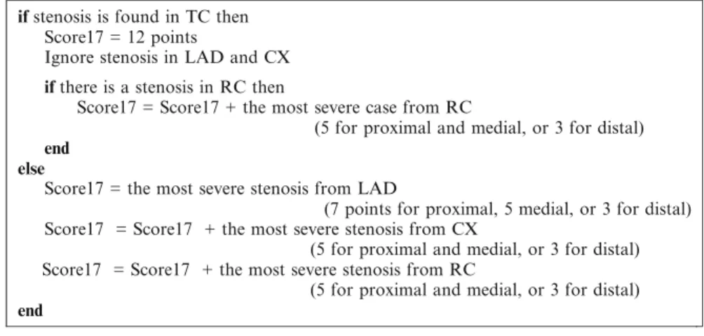
The more detailed special angiographic score proposed in [5] can be utilized for quantifying the severity of the disease. This score, herein denoted as Score17, assigns a severity level to a patient in the range of [0,. . .,17] with 17 being the most severe condition, while zero correspond to a normal patient. More specifically, this metric examines all the sites of the 4 major coronary arteries (e.g., the proximal, medial, and distal site of LAD) for lesions exceeding a predefined stenosis threshold. The exact computation of Score17 is presented in Fig.1.4.
Based on this score, four medically meaningful categories are defined: a. Score17¼0: Normal vessels
b. Score17 less or equal to 7: Mild ATS condition c. Score17 between 7 and 10: Moderate ATS condition d. Score17 between 10 and 17: Severe ATS condition
These can be used to directly set up a four-class problem denoted as S-vs-M-vs-M-vs-N. Furthermore, we defined a series of cases by grouping together the above subgroups, e.g., SM-vs-MN is the problem where the “Severe” class contains patients with severe ATS (case (a)) or moderate ATS severity (case (b)), while the mild and normal ATS diseased patients (cases (c) and (d)) constitute the “Mild” class. This definition is denoted as DefB.
1.3.4.3 HybridScore: A Hybrid Angiographic Score
Undoubtedly, Score17 gives more freedom to the specification of the target value of the problem. However, the need to define the threshold leads again in a large set of problem variants. To tackle this situation, we have developed an extension of this score that does not depend on a stenosis threshold. The basic idea is the use of a set of weights, each of them corresponding to different ranges of stenosis degree. These weights are incorporated to the score computation in order to add fuzziness to patient characterization. An example would explain the behavior of the modified Score17 denoted as HybridScore (Table1.3).
Examples:
a. Supposing that a patient has 50 % stenosis at TC, 50 % at RC proximal, 90 % at RC distal, and the rest of his vessels are normal, then the classic Score17, with a threshold at 75 % stenosis, assigns a disease severity level 3 for the DX distal stenosis.
ifstenosis is found in TC then Score17 = 12 points
Ignore stenosis in LAD and CX
ifthere is a stenosis in RC then
Score17 = Score17 + the most severe case from RC
(5 for proximal and medial, or 3 for distal)
end else
Score17 = the most severe stenosis from LAD
(7 points for proximal, 5 medial, or 3 for distal) Score17 = Score17 + the most severe stenosis from CX
(5 for proximal and medial, or 3 for distal) Score17 = Score17 + the most severe stenosis from RC
(5 for proximal and medial, or 3 for distal)
end
The developed HybridScore17 assigns 12*1/2(for TC) + max{5*1/2, 3*1}¼9. Note that for multiple stenoses at the same vessel, this score takes into account the most serious with respect to the combined weighted severity.
b. Let us examine another patient with exactly the same TC and RC findings, but having as well 90 % stenosis at LAD proximal and 90 % at CX medial. The traditional Score17 ignores these latter two, because they belong to the left coronary tree where TC is the most important part and exceeds the elementary threshold of 50 % stenosis (over which a vessel is generally considered as occluded). On the other hand, HybridScore17 would assign a severity value by computing the max {9(the previous result), 7 * 1(for LAD proximal) + 5 * 1(for CX medial)}¼12. Table1.4provides the values for the different CANGIO scores. For the Score17 the table provides the values with different stenosis thresholds: 50 % (T50), 75 % (T75), and 90 % (T90). Note also that the site of the stenosis might not reported by the medical expert during the examination. In these cases we assume that the stenosis is located at the proximal site (the most serious scenario). It is worth mentioning that the threshold of Score17 plays a crucial role in evaluating the ATS burden of a patient. In the eleventh line of Table1.4, we observe that using a threshold of 50 % stenosis, the score gives a value equal to 17 and with 75 % threshold the score is 12, while for 90 % threshold this value becomes 7. On the other hand, HybridScore is a single measurement with a value equal to 12.
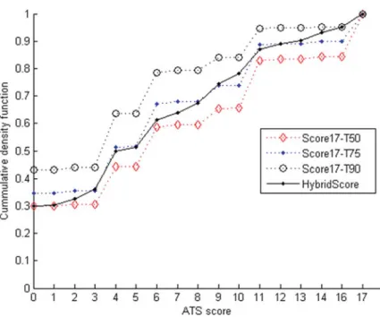
To illustrate the way the presented scores work, we provide the following graph that presents the cumulative density function (cdf) for the range of values 0–17, for the original Score17 using three different thresholds and the HybridScore. The scores have been computed for the 3,000 patient records of M-DB dataset. The value at ATS score¼0 corresponds to the number of patients that have a score value in [0,1], for ATS score¼1 a computed score in [0,1] or in [1,2], and so on. For example, looking at the Score17-T90 line, over 40 % of the 3,000 patients database are assigned with a score value equal to 0 and very few patients exist with score values larger than zero and less than or equal to 3. Apparently, there is a large group of patients (about 20 % of the total patients) that have a score over 3 and at most 4 (Figs.1.5and1.6).
Next, we present the respective figures, Figs.1.7and1.8, for the M-DB after excluding a subset of patients with a recorded history of PMI or AMI. These patients are generally cases of more serious ATS burden. This is depicted by the increased frequencies of the lower ATS scores in the cdf of Fig.1.7compared with the cdf in Fig.1.5of the full database of 3,000 patients.
To define a classification problem based on this angiographic score, a proper threshold needs to be specified. A value of HybridScore over that threshold would imply that a patient is severely diseased, and is mildly diseased, or even in normal condition, if his score is below threshold. This definition of ATS disease severity is denoted as DefC.
Table 1.3 The weights used
by the HybridScore Stenosis range <50 % 50–75 % 75–90 % 90–100 % Weight value 0 1/2 2/3 1
Table 1.4 The angiographic scores, Score17 for various stenosis thresholds and the proposed HybridScore, computed based on the CANGIO examinations of some patients of M-DB. When the site of a stenosis is not reported (e.g., for LAD and RC of the first patient), we assume that it is located at the proximal re gion of the artery CANGIO date Stenosed vessels ( 50 %) Main coronary arteries Score17 T50 Score17 T75 Score17 T90 Hybrid Score LAD CX RC TC Max P M D Max P M D Max P M D 19/11/1982 2 7 5 7 5 1 2 1 2 0 8.00 19/01/1983 3 7 5 7 5 7 5 7 5 5 0 5 0 1 3 8 0 7.83 13/12/1978 2 9 0 100 12 12 12 12.00 04/02/1983 1 100 100 7 7 7 7.00 14/01/1983 1 9 0 9 0 7 7 7 7.00 09/05/1979 2 9 0 7 5 1 2 1 2 7 10.33 03/11/2003 3 100 100 100 100 100 17 17 17 17.00 16/02/1983 1 9 0 7 5 9 0 5 5 5 5.00 16/02/1983 0 0 0 0 0.00 22/04/1983 2 9 0 9 0 9 0 9 0 1 2 1 2 1 2 12.00 02/03/1983 3 9 0 9 0 5 0 7 5 5 0 5 0 5 0 1 7 1 2 7 12.S3 06/03/2003 4 5 0 5 0 9 0 9 0 100 100 50 17 10 10 12.50 30/03/1983 3 9 0 9 0 9 0 7 5 9 0 9 0 9 0 1 5 1 5 1 3 13.33 20/04/1983 2 100 50 50 12 7 7 9.50 15/05/1979 3 100 90 75 75 17 17 12 15.33 14/11/2007 3 9 0 9 0 100 100 50 50 50 11 6 6 S.50 27/04/1983 3 9 0 9 0 7 5 7 5 7 5 7 5 7 5 1 7 1 7 7 13.67 09/03/1983 4 100 12 12 12 12.00
Fig. 1.5 The cumulative density functions of the Score17 and HybridScore for M-DB
Fig. 1.7 The cumulative density functions of the Score17 and HybridScore for M-DB, excluding the patients with PMI/AMI history
Fig. 1.8 The histogram of the different HybridScore values for M-DB, excluding the patients with PMI/AMI history (x-axis)
1.3.4.4 Discussion on Angiographic Scores
The introduction of the HybridScore proposed in this study has been proved very beneficial since it allows the complete characterization of the CANGIO examina-tion using a single numeric value, while the existing characterizaexamina-tion is using two numeric values (namely, Score17 and a stenosis threshold to compute the score). In this way it is straightforward to define the various classification problems that emerge by setting a threshold value (th) to this HybridScore (Mild class, hybrid score<th and Severe class, hybrid score>¼th). As the threshold value (th) increases from 0 to 17, we obtain a sequence of meaningful classification problems. The proposed HybridScore definition allows for the direct computation of the difference between two coronary examinations. To our knowledge, this is the first time such a difference is quantified in literature with a convenient measure which is also applicable for the quantification of ATS progression.
1.3.5
Results for Data Mining Tasks
This section will illustrate some of the results obtained during the analyses of the data in the described tasks. It should be noted that the presented results are provided as examples of the results that can be achieved by mining clinical data, and not as a facts that should be considered, or accepted, as having medical validity.
1.3.5.1 Correlating Patients’ Profile and ATS Burden
Data Preprocessing
In this task we used the information about the patients’ history and the first CANGIO examination. Initially, each patient record contains 70 features, some of them having missing values. For the nominal features that have missing values, we apply some of the feature transformations presented earlier in the chapter. • Binarize a Feature by Merging Rare Feature Values
For nominal features that take several values each of them having a very low frequency while at the same time having many missing values, we merge all existing different values to a “true” value, and the “false” value was assigned to the missing value cases. To be this transformation appropriate, the values that would be merged should express similar findings for the patient, i.e., all the values grouped into “true” should have similar medical meaning, all negative or all positive. An example is the feature describing the diagnosis for akinesia that takes values such as API (1.70 %), SET (0.97 %), INF (6.70 %), POS (0.23 %), LAT (0.13 %), ANT (0.03 %), and combinations of these values (14.96 %), while the rest 75.30 % are missing values. Apparently, all the reported values have the same negative medical meaning about negative findings diagnosed to the patients. In this case, the new
binary feature has 75.30 % the “true” value and 24.70 % the “false” value. Other similar cases are dyskinesia, hypokinesia, and AMI complications.
• Feature Extension for Nominal Features with Missing Values
Only one of the new binary features can be “true,” while a missing value is encoded as an instance where all these new features are “false.” This transfor-mation is used for features such as AMISTEMI and PMISTEMI.
Missing values are present for numeric features as well. To deal with these cases, we apply the following transformations:
• Firstly, we eliminated all such features that have a frequency of missing values over 11 %. These features were hdl (missing, 25.53 %), ldl (missing, 27.73 %), rpp (missing, 57.83 %), watt (missing, 57.87 %), septup (missing, 16.97 %), and posteriorwall (missing, 17.90 %).
• For the features that have less that 11 % missing values percentage, we filled them with the average feature value. This category of features includes hr (missing, 7.23 %), pressmin (missing, 1.20 %), pressmax (missing, 1.20 %), creatinine (missing, 9.70 %), cholesterol (missing, 6.60 %), triglic (missing, 8.63 %), and glicemia (missing, 10.53 %).
Special cases of features with missing values are the ejection fraction of the left ventricular of the heart (EF) and the diagnosis of a dysfunction of that ventricular (ECHO left ventricular dysfunction). These two findings are commonly measured by an electrocardiogram and are closely correlated since, usually, a dysfunction of the ventricle results in a low ejection fraction. The more serious a problem is diagnosed to the ventricle, the less fraction of the blood in the ventricle in end-diastole state is pumped out of the ventricle. In the M-DB, there are patient records where (a) both measurements are provided and (b) only one of the measurements is reported. We developed the heuristic procedure of Fig.1.9.
The final step of the above procedure applies feature expansion to the dysfunction of the ventricular. This is done in order to prepare the data for classification algorithms such as SVM, where the different nominal values cannot be handled. After the preprocessing we described, each patient record of the M-DB contains 92 features. This is the full set feature that we finally used.
(1) Compute the average and standard deviation for the EF values of each ventricular dys-function category (Normal, Regional, Global).
(2) Fill the missing EF values for patients without a dysfunction (Normal) cases with the av-erage EF value measured for the Normal patients. The same for the other dysfunctions (Regional and Global).
(3) Using the probability p(type of dysfunction | EF), computed assuming a Gaussian distri- bution to model the values of each dysfunction type, fill the missing dysfunction charac-terization based on the available EF value.
(4) Apply feature extension to Echo left ventricular dysfunction.
The AMI date was converted to an integer feature expressing the positive time difference in days between that date and the hospitalization date of the patient, similarly for the PMI date. The missing values of these features are filled with zeros. The results regarding the feature evaluation did not indicate that the elimination of certain features could lead to better predictions. In fact, there are some features that do not have much information associated with the value of the target variable that is predicted (the class of each patient) and are ranked in low positions, but, at the same time, when eliminated the performance of the models does not improve at all. Thus, we did not aim further on feature selection by means of computational feature evaluation. Instead, we considered a second version of each database for these two tasks where we discarded a number of features that are known to be medically high correlated with the ATS disease. This approach would force the training algorithms to use the remaining features and may reveal nontrivial connections between patient characteristics and the disease. The exact features discarded are ischemia at rest, AMI, AMI date, AMI STEMI (all the binary expansions), AMI NSTEMI, AMI complications, PMI, PMI date, PMI STEMI, PMI NSTEMI, history of CABG, history of PTCA, and ischemia on effort before (hospitalization). For AMI STEMI, AMI NSTEMI, PMI STEMI, and PMI NSTEMI, all the features of the feature expansion were eliminated. The set of features is then called “reduced.”
Evaluating the Trained Classification Models
In this task we aimed to build efficient systems that can discriminate the patients into two classes regarding the severity of their ATS disease condition that can be characterized as normal-mild or severe. In the previous section, we discussed how we can quantify the CANGIO examination into one single value using the proposed HybridScore. Based on that, we have defined the target variable for training classifiers. From the machine learning standpoint, we also need the value of the target variable for each patient, i.e., the indication about the class each patient belongs. Unfortunately, this requires medical knowledge about specific values of the ATS scores that could be used as thresholds. This cannot be provided since there are not any related studies in the literature that propose such a cutoff value. In fact one could make reasonable choices but there is no gold standard to use.
As a result, we should test all possible settings of ATS score and build classifiers for all these cases. For example, we choose to use all integer values of the HybridScore in [0,17]. Then we need to evaluate the classifiers produced for a fixed classification problem, with a specific cutoff threshold. An evaluation of the produced classifiers is also needed in a second level: to understand which classification is medically more meaningful or easier to solve based on the available data. In other words, the objectives of the analysis are both to find the interesting discrimination problems as well as to find interesting solutions for them. In fact, this is a complex procedure where the final classifiers are somehow evaluated by both supervised and unsupervised way. And this is the most challenging issue we had to deal with in this study.
Supposing we have produced all classifiers for all thresholds of HybridScore, we evaluate the produced system using multiple quality indicators. The first category of
indicators is the classification accuracy and indices such as kappa statistic. Different classifiers trained on the same target values (same threshold) can be directly compared in terms of their classification accuracy measured using cross-validation. On the other hand, if two classifiers have been trained on different values of the target variable, then it is not trivial to compare them in a strict way.
Thus a different level in which we examine how interesting each specific classifier is compared to other classifiers produced for different HybridScore thresholds is to measure the gain in classification accuracy they present with respect to an “empty-box” decision system that decides always for the largest class of patients in every case. For instance, let us consider a discrimination problem with 60 % seriously diseased patients and 40 % normal-mild cases for which a classifier gives 75 % prediction accuracy. Let us consider the second problem with 80–20 % distribution of patients and a respective classifier achieving 82 % accuracy. We can conclude that the first system with 15 % gain in accuracy retrieves a greater amount of information from the available classes compared to the 2 % of the second one.
The class distribution is also called “class balance” and is an important determi-nant for most of training algorithms. When one of the classes is overrepresented in a training set, then the classification algorithm will eventually focus on the larger data class and probably will lose the fine-detail information in the smaller class. To this end, we adopted an additional evaluation strategy for the classification problems. In particular, we selected all the patients from the smaller class and an equal number of randomly selected patients from the larger class to train a classifier. This is repeated five times and the reported accuracy is the average accuracy of the five classifiers. This approach is denoted as “Balanced.” Secondly, we select at most 200 patients from the two classes and follow the previous workflow. This strategy is called “Balanced200.” The second strategy may reveal how a classifier scales to the size of database, the number of patients provided for training, in a problem with a fixed HybridScore threshold. If the accuracy does not drop dramatically when fewer patients are used for training, then this is an indication of getting stable results. Note that this is only an evaluation methodology since the final classifiers we created were trained on the full dataset at each time, for the selected class definition.
Classification Results
Defining ATS Disease Severity Using DefA
According to the ATS severity definition DefA, which combines the number of diseased vessels and the stenosis level, we trained classifiers for all possible discrimination problems that could be set. In Fig.1.10we used the SVM classifiers to evaluate the different discriminating problems. The last one considers the normal or mildly diseased patients to be those with at most two arteries with at most 75 % stenosis. The green line indicates the size of the largest class in each definition of the mild-severe classes. The brown line is the SVM accuracy on all the data of the M-DB, and the blue is the gain in accuracy, i.e., the difference between the SVM accuracy and the largest class (green line). The large gain values indicate the settings under which the classifier managed to retrieve much more information from the data than that of the empty-box classifier.
The gain might be increased for mainly two possible reasons. The first is the fact that the problem setting we considered is more separable comparing to the other settings. Thus the data properties (the characteristics of patients) are better described by this specific class definition, and this also indicates that it is interesting to understand the properties that led to this classification grouping “preference.” The second reason might be the class balance. When classes are balanced in size, the classifier may achieve lower accuracy value, but still with remarkable gain. This is the role of the experiments we do on balanced subsets of the M-DB. The deep blue line shows the average accuracy of the SVM for the 5 balanced data subsets, and the red is the balanced case of 200 patients per class. If these two lines are close enough in performance, it is evident that the classification performance is not heavily dependent on the amount of available data (similarly one could state that the classifier retrieves as much information as the data let under the specific class definition).
Having all these in mind, we can look back in Fig. 1.10 to observe that the balanced class definitions clearly indicate the first three cases as the best out of all. In particular, the first one, defining the severe class as having all patients with at least one artery with at least 90 % stenosis level, is the overall best since the class sizes of the full DB are more balanced. Table1.5summarizes the classification results for all the patients and features of M-DB. The largest class is indicated as Fig. 1.10 Classification results using SVM for different definitions (DefA) of discrimination problems on M-DB
Table 1.5 Classification results using definition DefA for ATS disease severity. All patients and features are used Problem description Accuracy Kappa Gain Diseased arteries Largest class DT-J48 Random Linear SVM J48 RF Linear SVM number (stenosis) size (%) class All (size) Forest All Bal Bal200 All All All All Bal Bal200 > ¼ 1( > ¼ 90 %) 60.23 (S) 72.50 (06/11) 74.23 75.57 73.21 71.55 0.4102 12.27 14.00 15.34 23.21 21.55 > ¼ 1( > ¼ 75 %) 69.00 (S) 76.73 (10/19) 78.73 80.07 75.34 74.90 0.4054 08.60 09.73 11.07 25.34 24.90 > ¼ 1( > ¼ 50 %) 73.80 (S) 79.00 (09/17) 81.53 82.70 74.55 75.55 0.3910 05.90 07.73 08.90 24.55 25.55 > ¼ 2( > ¼ 90 %) 77.63 (M) 81.13 (02/03) 79.93 81.23 69.21 65.80 0.2834 02.40 02.30 03.60 19.21 15.80 > ¼ 2( > ¼ 75 %) 65.08 (M) 70.83 (09/17) 70.60 71.23 67.26 65.30 0.2560 05.45 05.52 06.15 17.26 15.30 > ¼ 2( > ¼ 50 %) 56.70 (M) 66.03 (07/13) 66.90 69.00 68.75 69.00 0.2781 10.06 10.20 12.30 18.75 19.00 > ¼ 3( > ¼ 90 %) 93.50 (M) 93.5 (01/01) 93.50 93.50 71.28 69.74 0.0000 00.00 00.00 0.000 21.28 19.74 > ¼ 3( > ¼ 75 %) 88.10 (M) 87.8 (05/09) 88.23 88.10 67.56 68.40 0.1163 00.30 00.13 00.00 17.56 18.40 > ¼ 3( > ¼ 50 %) 81.60 (M) 81.57 (16/31) 82.23 82.10 64.93 66.15 0.1271 00.03 00.63 00.50 14.93 16.15 < ¼ 2( > ¼ 75 %) 90.23 (S) 90.23 (01/01) 90.20 90.23 63.96 63.00 0.1763 00.00 00.03 00.00 13.96 13.00
Severe (S) or Mild (M); the size of a decision tree (DT) is denoted as (number of leaves/number of total tree nodes). The performance of random forest (RF) and SVM is also reported. The three different evaluation indices are denoted in the first line: accuracy, kappa statistic, and accuracy gain. “Bal” indicates the subset of the M-DB with balanced data classes, and “Bal200” are subsets that contain balanced classes with at most 200 patients each. The k-statistic also indicates that in the first three cases, the DT J48 retrieves the “real structure” of the data defined by the considered class labels for the patients.
The DT corresponding to the first line of Table 1.5is presented in Fig.1.11. The quality of a rule is indicated by the two numbers inside the rectangle leaf, the first is the number of patients that this leaf decides for and – after the “/” character – the number of patients that were incorrectly classified in the class of the leaf.
References
1. M.W. Browne, “Cross-validation methods”, Journal of Mathematical Psychologyvol. 44, Issue 1, pp. 108–132, March 2000.
2. I.H. Witten, Eibe Frank, “Data Mining: Practical Machine Learning Tools and Techniques”, Morgan Kaufmann, June 2005.
3. R. Herbrich, Learning Kernel Classifiers, MIT Press, Cambridge, MA, 2002.
4. I. Guyon and A. Elisseeff, “Variable and feature selection”, Journal of Machine Learning Research, vol. 3, March 2003.
Pos =0 >0 Sex Severe (210/11) History of CABG Pos Neg Neg Pos Neg Male Female Regional LV dysfunction Severe (998/234) Severe (240/68) Severe (522/167) Mild (278/110) Mild (752/207) PMI STEMI number Angina on effort Fig. 1.11 The DT for the
classification problem that considers the ATS condition of a patient as severe when he has at least 1 artery with at least 90 % level of stenosis
5. A. Gimelli, G. Rossi, P. Landi, P. Marzullo, G. Iervasi, A. L’Abbate, and Daniele Rovai, “Stress/Rest Myocardial Perfusion Abnormalities by Gated SPECT: Still the Best Predictor of Cardiac Events in Stable Ischemic Heart Disease”, Journal of Nuclear Medicine, vol. 50, Issue 4, April 2009.
6. I. Guyon, J. Weston, S. Barnhill, V. Vapnik, “Gene Selection for Cancer Classification using Support Vector Machines”, Machine Learning, vol. 46, Issue 1–3, pp. 389–422, 2002. 7. University of California – Irvine (UCI) Machine Learning Repository: http://archive.ics.
uci.edu/ml.
8. R. Das, I. Turkoglu and A. Sengur, “Effective Diagnosis of Heart Disease through Neural Network Ensembles”, Expert Systems with Applications, vol. 36, pp. 7675–7680, 2009. 9. M.G. Tsipouras, T.P. Exarchos, D.I. Fotiadis, A.P. Kotsia, K.V. Vakalis, K.K. Naka,
L.K. Michalis, “Automated Diagnosis of Coronary Artery Disease Based on Data Mining and Fuzzy Modeling”, IEEE Transactions on Biomedical Engineering, vol. 12, Issue 4, pp. 447–458, 2008.
10. C. Ordonez, “Comparing Association Rules and Decision Trees for Disease Prediction”, Proceedings of the ACM HIKM’06, Arlington, 2006.
11. C. Ordonez, N. Ezquerra and C. Santana, “Constraining and Summarizing Association Rules in Medical Data”, Knowledge and Information Systems, vol. 9, Issue 3, pp. 259–283, 2006. 12. P. Chanda, L. Sucheston, A. Zhang, D. Brazeau, J.L. Freudenheim, C. Ambrosone and
M. Ramanathan, “AMBIENCE: A Novel Approach and Efficient Algorithm for Identifying Informative Genetic and Environmental Associations with Complex Phenotypes”, Genetics, vol. 180, pp. 1191–1210, October 2008.
13. J.H. Moore, J.C. Gilbert, C.T. Tsai, F.T. Chiang, T. Holden, N. Barney and B.C. White, “A flexible computational framework for detecting, characterizing, and interpreting statistical patterns of epistasis in genetic studies of human disease susceptibility”, Journal of Theoretical Biology, vol. 241, pp. 252–261, 2006.
14. International HapMap Project:http://hapmap.ncbi.nlm.nih.gov/abouthapmap.html
15. J. R. Quinlan and J. R. C4.5, “Programs for machine learning”, Morgan Kaufmann Publishers, 1993.
16. C. Cortes and V. Vapnik, “Support-vector network”, Machine Learning, vol. 20, Issue 3, pp. 273–297, 1995.
17. N. Cristiannini and J. Shawe-Taylor, “An Introduction to Support Vector Machines and Other Kernel-Based Learning Models”, Cambridge University Press, 2000.
18. L. Breiman, “Random Forests”, Machine Learning, vol. 45, Issue 1, pp. 5–32, 2001. 19. P. Tan, M. Steinbach and V. Kumar, “Introduction to Data Mining”, Addison-Wesley, 2005. 20. T. Hastie, R. Tibshirani and J. Friedman, “The Elements of Statistical Learning”,
Springer-Verlag, 2008.
21. H. Liu and R. Setiono, “Chi2: Feature selection and discretization of numeric attributes”, Proceedings of the IEEE 7th International Conference on Tools with Artificial Intelligence, pp. 338–391, 1995.
22. H. Peng, F. Long, and C. Ding, “Feature selection based on mutual information: criteria of max-dependency, max-relevance, and min-redundancy”, IEEE Transactions on Pattern Anal-ysis and Machine Intelligence, vol. 27, Issue 8, pp. 1226–1238, 2005.
23. A. Reiner, C. Carlson, B. Thyagarajan, M. Rieder, J. Polak, D. Siscovick, D. Nickerson, D. Jacobs Jr, and M. Gross. “Soluble P-Selectin, SELP Polymorphisms, and Atherosclerotic Risk in European-American and African-African Young Adults”, Arteriosclerosis, Thrombo-sis and Vascular Biology, August 2008.
24. A. Timinskas, Z. Kucinskiene, and V. Kucinskas. “Atherosclerosis: alterations in cell commu-nication”, in ACTA MEDICA LITUANICA, vol. 14, Issue 1. P. 24–29, 2007
25. S. Szymczak, B.W. Igl, and A. Ziegler. “Detecting SNP-expression associations: A compari-son of mutual information and median test with standard statistical approaches”, Statistics in Medicine, vol. 28, pp. 3581–3596, 2009.