Essays on temporary migration

(1)

Essays on Temporary Migration

Josep Mestres Dom`enech

A dissertation submitted to the Department of Economics in partial fulfillment of the requirements for the degree of

Doctor of Philosophy

of the

University College London.

(2)

2

I, Josep Mestres Dom`enech confirm that:

• the work presented in this thesis is my own and it has not been presented to any other university or institution for a degree.

• where information has been derived from other sources, I confirm that this has been indicated in the thesis.

• chapter two is based on cojoint work with J´erˆome Adda (European University Institute) and Christian Dustmann (University College London).

• chapter three is based on cojoint work with Christian Dustmann (University Col-lege London).

• chapter four is based on cojoint work with Christian Dustmann (University Col-lege London).

(3)

Abstract

My thesis dissertation focuses on the temporariness of migration, its diverse effects as

well as on migration selection.

The first paper, A Dynamic Model of Return Migration analyzes the decision

pro-cess underlying return migration using a dynamic model. We explain how migrants decide whether to stay or to go back to their home country together with their savings

and consumption decisions. We simulate our model with return intentions and perform policy simulations.

The second paper, Remittances and Temporary Migration, studies the remittance behaviour of immigrants and how it relates to temporary versus permanent migration

plans. We use a unique data source that provides unusual detail on the purpose of remittances, savings, and return plans, and follows the same household over time. Our

results suggest that changes in return plans lead to large changes in remittance flows. The third paper, Savings, Asset Holdings, and Temporary, analyzes how return

plans affect not only remittances but also savings and the accumulation of assets. We show that immigrants with temporary return plans place a higher proportion of savings

in the home country and have accumulated a higher amount and share of assets and housing value in the home country (compared to the host country).

Finally, the fourth paper, Migrant Selection to the U.S.: Evidence from the Mex-ican Family Life Survey (MxFLS), studies the selection in terms of skills of recent

migrants to the United States using the MxFLS. We highlight the important age gra-dient of migration, the different education attainment between age cohorts in Mexico

and show the implications when analyzing migrant selection. Our claim is that in order to properly study the self-selection of migrants, it is necessary to compare migrants to

(4)

Acknowledgements

My deepest gratitude to my supervisors Christian Dustmann and J´erˆome Adda. I highly

appreciate their encouragement and guidance during all these years. It has been an in-valuable experience to work together on several projects and to take part in the

organi-zation of the CReAM center.

I am very grateful as well to the rest of professors at CReAM and the Economics

Department in UCL for their teaching and advice during my PhD. All the members of the UCL Economics department made my time there an exciting one.

I would also like to thank my colleagues at CReAM and fellow PhD students at UCL. Albrecht Glitz, Anna Raute, Anna Rosso, Andreas Uthemann, Carolina

Or-tega, Caroline Thomas, Ciro Avitabile, Claudia Trentini, Cristina Santos, Daniele Con-dorelli, Fabio Michelucci, Francesco Fasani, Katrien Stevens, Mario Fiorini, Matti

Sarvimaki, Matthias Parey, Panu Pelkonen, Thomas Cornelissen, Tom Rutter, Tom-maso Frattini,... all our discussions and experiences together have been very enriching.

The permanent support of all my family and friends has been as important. William has supported me unconditionally, even after leaving London. My mother

and sisters have encouraged me from the beginning until the end. And all my friends who helped me, even from abroad: Claudia Canals, Darja Debevec, Gonul Dogan,

Ju-dit Montoriol, Marta Felis, Melanie Luhrmann, Miriam Morath, Montse Duran, Pepita Miquel, Simone Kohnz,... just to name a few. Many thanks to all of you.

(5)

List of Tables

2.1 Summary Statistics . . . 31

2.2 Variations in return plans . . . 32

2.3 Differences between intention to return in 1984 and actual return (prior to 2007) . . . 35

2.4 Calibrated coefficients . . . 39

3.1 Summary Statistics - 1984-1994 . . . 64

3.2 Remittances by Household Characteristics . . . 65

3.3 Distribution of Household Remittances . . . 66

3.4 Probability to Remit and Amount Remitted - OLS . . . 67

3.5 Probability to Remit and Amount Remitted - Fixed Effects and GMM . 68 3.6 GSOEP Data Availability . . . 69

3.7 Probability to Remit - Full Set of Results . . . 70

3.8 Amount Remitted - Full Set of Results . . . 71

3.9 Amount Remitted Conditional on Remitting - Full Set of Results . . . . 72

4.1 Summary Statistics . . . 91

4.2 Savings, Home Ownership and Assets . . . 92

4.3 Savings - Home and Host Country . . . 93

4.4 Property Ownership - Home and Host Country . . . 94

4.5 Asset Holdings - Home and Host Country . . . 95

4.6 Total Savings . . . 96

4.7 Total Property and Asset Holdings . . . 97

(8)

List of Tables 8

5.2 Number of Years of Education - Distribution Among Migrant and

Non-Migrant Mexicans . . . 117

5.3 Educational Level - Distribution Among Migrant and Non-Migrant Mexicans . . . 118

5.4 Wages in Mexico in 2002 - Distribution Among Migrant and Non-Migrant Mexicans . . . 119

5.5 Raven’s Test Score - Distribution Among Migrant and Non-Migrant Mexicans . . . 122

5.6 Male Descriptives . . . 123

5.7 Female Descriptives . . . 124

5.8 Raven’s Test Score - OLS Regression . . . 125

5.9 Alternative Young Definition (12-36) - Number of Years of Education, Log Wages and Ravens Test Scores Distributions Among Migrant and Non-Migrant Mexicans . . . 126

5.10 Alternative Young Definition (20-29) - Number of Years of Education, Log Wages and Ravens Test Scores Distributions Among Migrant and Non-Migrant Mexicans . . . 127

(9)

List of Figures

2.1 Inflows and outflows of migrants in Germany by selected countries of

origin, 1968-2008 . . . 30

2.2 Changes in return intentions (difference in years) . . . 33

2.3 Intentions of migrants over time . . . 34

2.4 Difference in years between intended and actual stay durations . . . 36

2.5 Distribution of Migration Intentions . . . 37

2.6 Distribution of Migration Intentions by Duration of Stay . . . 38

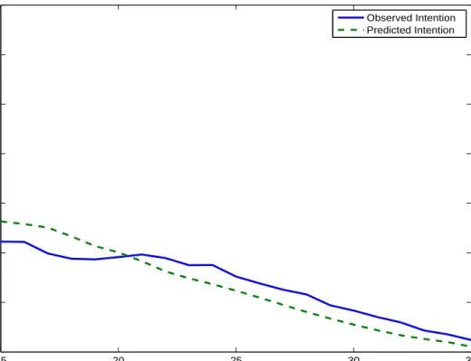
2.7 Observed Intention vs. Predicted Intention - Individual Aged 35 and 15 Years Since Migration . . . 40

2.10 Effect of subsidy to return to home country . . . 43

2.11 Effect of change in relative income . . . 44

2.12 Effect of different home country economic conditions . . . 45

5.1 Age Distribution Boxplot - Mexican Non-Migrant vs. Migrant . . . 115

5.2 Educational Attainment in Mexico over time (1970-2005), by age groups. . . 116

5.3 Wages in Mexico in 2002 - Distribution Functions of Migrant and Non-Migrant Mexicans . . . 120

5.4 Wages in Mexico in 2002 - Differences in Distribution Functions be-tween Migrant and Non-Migrant Mexicans . . . 121

(10)

Chapter 1

Introduction

Migration is the result of a rational process. Individuals decide to leave their

coun-tries after assessing the potential benefits and costs of such decision. The decision on whether to return or not is the result of a rational calculation, as the initial migration

de-cision was. We analyse in this thesis the potential temporariness of migration and study how migrants assess it. In addition, we show how migrants modify their behaviour in

the host country depending on their migration return intentions. Finally, we focus on migrants’ selection in terms of skills, its correct assessment and the implications it

might have.

Chapter 2 analyzes the decision process underlying return migration using a dy-namic model. In each period, migrants decide whether to stay in host country or to

return to home country, simultaneously with consumption and investment choices. The decisions are taken comparing the discounted flow of utility between staying for an

additional year and returning to the home country permanently, and depend on the cap-ital invested in each country as well as on a series of stochastic shocks. The dynamic

model framework allows migrants to revise their decisions in each period, given shocks in preferences for the home country and shocks in the relative income between the host

country and the home country. We use the German Socio-Economic Study (GSOEP) panel data, which allows us to follow migrants from different countries for a period of

24 years. It also reveals their return intentions in each time period and whether they return or not. We calibrate our model of return intentions and perform several policy

simulations. Our policy simulations illustrate the importance of economic prospects of the home country on modifying migrants’ intentions to return to their home country,

(11)

11

It is important to understand migrants’ intentions not only for its own sake.

Re-turn intentions modify as well migrants’ behaviour while in the host country, and this issued is analyzed in chapters 3 and 4. Chapter 3 studies how the intended stay in the

host country (or the potential return to the home country) modify migrants’ remittance behaviour. We use the GSOEP data that provides unusual detail on remittances and

return plans, and follows the same household over time. Our data allows us also to distinguish between different purposes of remittances. We analyze the association

between individual and household characteristics and the geographic location of the family as well as return plans, and remittances. The panel nature of our data allows

us to condition on household fixed effects. To address measurement error and reverse causality, we use an instrumental variable estimator. Our results show that changes in

return plans are related to large changes in remittance flows.

Return plans affect not only remittances but also savings and asset accumulation. These issues are analyzed in Chapter 4 using the GSOEP dataset. We argue that not

only the amount of savings and assets may be related to future return plans accumu-lation, but also if savings and assets are held in the home- and host country. Thus,

comparing savings and assets between immigrants and natives may lead to serious underestimation when neglecting the home country component. We show that

immi-grants with temporary return plans place a higher proportion of their savings in the home country. In addition, both the magnitude and the share of assets and housing

value accumulated in the home country are larger for immigrants who consider their migration as temporary, and lower the value of assets and property held in the host

country. These decisions might have important implications for both home and host countries’ asset and housing markets. Finally, and conditional on observable

character-istics, we find no evidence that immigrants with temporary migration plans save more than immigrants with permanent migration plans.

The last topic we analyse in this thesis is the selection in terms of skills of recent migrants to the United States in chapter 5. Migrants are self-selected in terms of skills

(12)

12

selection has important implications for both countries as the impact of migration on the non-migrant population depends on it. In this chapter we stress the important age

gradient of migration, the different education attainment between age cohorts in Mexico and show the implications when analyzing migrant selection. Our results show that

it is necessary to compare migrants to non-migrants of the same age cohort in order to properly analyse the self-selection of migrants. Our study shows that young male

migrants from Mexico are negatively selected in terms of education, wages and test scores, which affects the impact their migration has in both host and home countries.

(13)

Chapter 2

A Dynamic Model of Return

Migration

∗

(14)

2.1. Introduction 14

2.1

Introduction

The theoretical and empirical literature on migration has paid little attention to the fact

that many migrants return to their home countries after having spent a number of years in the host country. This is surprising, since many migrations today are in fact

tem-porary. For instance, labor migrations from Southern to central Europe in the 1950’s – 1970’s were predominantly temporary. Bohning (1987) estimates that ”more than

two thirds of the foreign workers admitted to the Federal Republic [of Germany], and more than four fifth in the case of Switzerland, have returned”. Glytsos (1988) reports

that of the one million Greeks migrating to West Germany between 1960 and 1984, 85% gradually returned home. Dustmann (1997) provides evidence for a substantial

out migration over that period for other European countries. Return migration is also considerable for the United States. Jasso & Rosenzweig (1982) report that between

1908 and 1957 about 15.7 million persons immigrated to the United States and about 4.8 million aliens emigrated. They found that between 20% and 50% of legal

immi-grants (depending on the nationality) re-emigrated from the United States in the 1970’s. Warren & Peck (1980) estimate that about one third of legal immigrants to the United

States re-emigrated in the 1960’s. Re-emigration rates in the United States and in sev-eral European countries were estimated to be between 20% to 60% during the 1990’s

(OECD (2008), Dustmann & Weiss (2007)).

To understand the motives of return migrations, as well as the factors which

ex-plain variation in migration durations, is important for designing optimal migration policies. The large labour migrations to Europe in the 1950’s to 1970’s were thought

to be temporary by the receiving countries and, in fact, many of these migrants did eventually return.

Most countries want to attract the best workers for their local labour markets and want to put in place migration schemes that allow them so do so. Furthermore, there

seems to be an understanding that it is desirable that these workers adopt easily to the social and economic structure of the host country. From the side of the migrant, the

in-centive for any migration, as well as the inin-centives to assimilate are heavily interrelated with the expected duration in the host region.

Little is known about the way migrants form their re-migration decisions. While

(15)

are wage differentials between regions, re-migrations occur despite persistently more favourable conditions in the host countries. Models which explain re-migrations must

therefore introduce non-monetary aspects which explain return migration, or deviate from absolute measures of monetary wealth, consider decisions taken within family

units, or take a more dynamic perspective, where intertemporal substitution is a driving force for return decisions.

The explanations found in the literature explaining why a return migration may be

optimal, despite persistently more favourable conditions in the host country, build on such considerations. Stark & Taylor (1991) uses the theory of relative deprivation and

arguments of risk spreading to explain why migrants may return to a less rich econ-omy or region. Djajic & Milbourne (1988) explain return migration by assuming that

migrants have a stronger preference for consumption at home than abroad. Dustmann (1999) shows that return migration may be optimal if the host country currency has

a higher purchasing power in the home country, and if there are higher returns in the home economy on human capital, acquired in the host country.

None of these models allow for revisions of return plans during the migrants’ migration history. They usually assume that the migrant has full information about the

host country, and that no unforseen shocks occur. Although these models give us some insight into the factors which are responsible for re-migration decisions, they seem to

leave out two very important elements. First, habituation processes, which may lead the migrant to revise former migration plans in the course of his/her migration history.

Second, shocks, or new information, which may lead the migrant to continuously revise previous migration plans. To appropriately address these issues is only feasible in a

dynamic setting, where migration plans and their revisions are modeled explicitly.

In this paper, we develop a dynamic model of return migration. Migrants make

a decision each period whether to stay in the host country or to return to the country of origin. The decisions taken are based on a comparison of the discounted flow of

utility in the two locations and depend on the capital invested in each country, as well as on a series of stochastic shocks. On the one hand there is a country specific shock

(16)

country. On the other hand, there are shocks specific to the individual, which allow for different stochastic influences across individuals. Migrants are allowed to re-optimize

their choices at every period after they have migrated. This feature is realistic: migrants revise their plans during the migration history. There are many reasons that might

mo-tivate them to do so, such as changes in his preferences for staying in host country due to habituation or unexpected changes in income.

Understanding the process of migrants’ re-migration decisions is not only

impor-tant for its own sake, though. The mere fact that some immigrants plan to return, while others do not, induces heterogeneity in their behaviour, like remittances (see chapter 3

), savings and asset accumulation (see chapter 4), labour market behaviour, skill

accu-mulation, consumption, etc. This heterogeneity is a consequence among others of the different economic situations they face after a return to their home countries, and which

they take into account when making current economic decisions. These differences in plans may help to explain, for instance, differences in assimilation patterns between

immigrant populations with different origin, as found in a number of empirical studies1.

There is some research on the effect of return plans on migrants’ behavior. Djajic (1989) emphasizes that in a guest worker system, changes in wages and prices in the

home country affect the migrant’s consumption and labor supply in the host country. Galor & Stark (1990), Galor & Stark (1991) show that a return probability different

from zero affects migrants’ behavior and performance in the host country, if wages in the home country differ from those in the host country. These models assume that

re-turn decisions are exogenous, and not optimally chosen by the immigrant. Dustmann (1999) builds a model where human capital accumulation in the host country, and

re-turn migrations, are both chosen simultaneously. Dustmann (2000) explores the conse-quences for the empirical analysis of migrants’ wage growth. If re-migration is chosen

optimally, then empirical models which do not condition on the migration duration are misspecified, and may lead to biased parameter estimates.

Again, the process of forming return plans is modeled in a simplistic way. In our framework, where migrants may constantly revise their return plans, it is possible to

(17)

2.2. Data and Some Evidence on Return Migration 17

update past return plans given new information or shocks. In this way, return plans are optimally chosen every period. From the perspective of the migrant and the host

country, this revision is desirable to avoid an incorrect assessment of migrants’ planned duration of stay in the host country.

2.2

Data and Some Evidence on Return Migration

Many migrations nowadays are temporary. On average, four in ten long-term migrants leave their host countries and re-migrate after five years of residence (OECD (2008)).

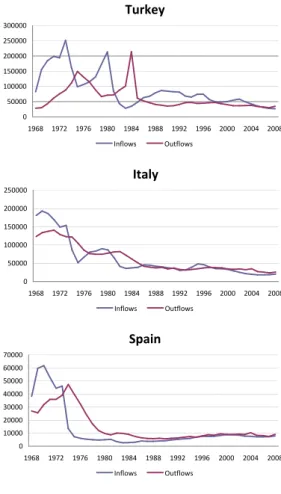
For the case of Germany, a large number of migrants enter the country and a large number also leave it. Figure 2.1 shows inflows to and outflows from Germany during

the last forty years (1968-2008) for migrants from different countries of origin. The fluctuation patterns of both inflows and outflows are different for migrants from

dif-ferent countries of origin. This might suggest that home country specific economic conditions matter in migration decisions, both to emigrate from the home country but

also to return to it.

In this paper, we use data from the first 24 waves of the German Socio-Economic Panel (GSOEP) for the years 1984 until 2007. This data set contains a boost sample of

immigrants (including some 1500 households in the first wave) from the former labour migration countries Spain, Italy, Greece, Yugoslavia, and Turkey. Migrants from these

countries were actively recruited during the late 1950’s - early 1970’s. Migrations were intended to be temporary both by the immigrant, as well as by the German authorities.

However, no temporary residence permits were imposed, and migrants could stay per-manently, if they wanted.

Our data has detailed information on individual characteristics, family back-ground, and economic activities of migrants over the 24 years period. Furthermore,

each year there was a complementary survey addressed to immigrants about various immigrant specific issues. One question refers to the migrant’s return plans. We define

as a temporary migrant those who want to return to their home country at some point in the future. The migrant is asked whether s/he intends to return to the home country,

(18)

do you want to live in Germany?” and the respondent can answer ”I want to remain in Germany permanently”, ”I want to return within the next 12 months” or ”I want to

stay several more years in Germany”. For the last option, he can state the ”number of years” he wishes to stay in Germany. Thus, in addition to the information regarding the

intention whether or not to return home, the sample also contains information about the intended remaining time in the host country, in case migrants would like to return2_{, and}

the completed migration spells until year 2007 for those who returned.

We provide some descriptive information about our data in table 2.1. In 1984, im-migrants are on average 35 years old and have stayed in Germany for about 13 years.

More than 70 percent intend to stay in Germany only for a temporary period of time (on average, 18 years) and return afterwards to their home country. The proportion of

individuals in the sample that wants to return decreases over time, due to both sam-ple selection and changes in return intentions. Of those who were in the samsam-ple in

1984, almost one quarter returned back to their home country at some point during the observational period (1984-2007).

Migrants change their return plans also during their stay in Germany. In table 2.2

we display cross-tabulations of intentions in subsequent years, where vertical entries refer to yeart and horizontal entries to yeart−1. Of those who intended to return in yeart−1, about 82% still have the same intention in yeart, but about 18% do not intend to return any more in yeart. Of those who did not want to return int−1, almost one quarter want to return in yeart. This indicates the existence of substantial fluctuations in return plans over the migration cycle.

In addition, the intended duration of stay changes over the migration experience.

If a deterministic model was appropriate for explaining return plans, then responses should be updated each year in a mechanical manner. For instance, if an individual

responds in yeart to have the intention to remain for 5more years abroad, then s/he should respond in yeart+ 1that s/he intends to remain only 4 more years, etc. This

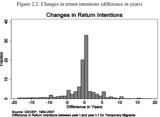
pattern does clearly not occur in our sample. Figure 2.2 shows the changes in the length of stay in the host country between one year and the following for those migrants

that declare their intention to return in both dates. We should observe all observations

2_{In case migrants intend to remain permanently, we will define the intended remaining time in the}

(19)

concentrated around −1 if intentions were updated in a deterministic way. This is clearly not the case for everyone. Only 20 percent update their intended stay in a

deterministic manner, while more than 30 percent declare the same intended stay int andt+ 1 and almost 50 percent update their intentions in a different manner. Those

individuals that declare the same intended stay intand int−1might include individuals who do not update their intentions because they answered quickly a probable return date

using an heuristic information process (instead of a systematic one), without making a proper assessment when to return analyzing all alternatives, etc.

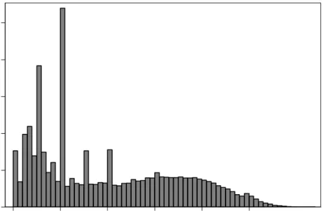
An additional example of how intended duration of stay is updated over the migra-tion experience can be observed in Figure 2.3. The figures shows the intended duramigra-tion

of stay of individuals who were still in Germany in 2007 during the migration history. We can see how the intended duration of stay is modified during the stay in the host

country and not in a deterministic way. In fact, the average intended stay even increases in the first years since migration, to start decreasing over time afterwards.

As mentioned previously, GSOEP also has information on completed migration

spells. If migrants drop out of the panel because they return to their home country, this information is recorded in the next wave of the panel. This allows us to compare return

intentions in 1984 (the first year the data is collected) and the actual returns until 2006 - see table 2.3. Of those who planned to return in 1984, almost 30 percent did indeed

go back over the next 23 years. Of those who did not intend to return, 14 percent did in fact go back over the next 23 years period. These numbers indicate that intentions and

realizations may vary quite considerably over the migration cycle.

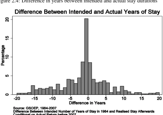
We can compare as well the difference in years between intended and actual stay

durations for those who returned before 2007. The differences between their intended return date and their actual return date are remarkable (figure 2.4). More than half

of the migrants who returned before 2007 declared in 1984 an intended time of stay Germany close to their actual stay (plus or minus three years). However, almost half

of the migrants either underestimated or overestimated their stay by more than three years.

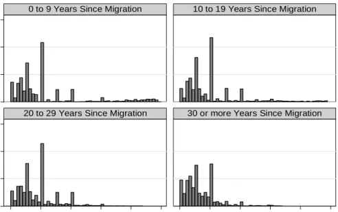
The distribution of intended stay in the host country is shown in Figure 2.5. Around 75 percent of those individuals that want to return intend to do so in the

(20)

2.3. The Model 20

of stay (e.g., 5 years, 10 years, 15 years, etc), as they might not know with certainty at which exact date they plan to return. The distribution of intended stay in the host

coun-try varies as well with duration of stay (Figure 2.6). Those individuals that recently arrived to the home country (between 0 to 9 years since migration) are more likely to

report longer intended stays than those who have already stayed in the host country for longer and still want to return to their home country. In all categories, nevertheless,

migrants are more likely to give round numbers as intended stay durations.

2.3

The Model

In our model, the agent has in every period a choice of location between his country of origin and the host country. Returning to his/her country of origin is a permanent

decision. In either of these locations, he derives a specific utility, which depends on expenditures in that location, and the time spent there. At each period in time, the

agent allocates his income into consumption,cand savings,s. The stock of savings,S is transferable across countries.

LetV(A, G, Y, λ, S, ηS, ηR) be the lifetime value of an individual of ageA, who

has been in the host country forGyears and with a stock of assetS. Y is the GDP in

the home country, relative to the host country. λis a shock to preferences, while in the host country. ηS andηR are two taste shocks, assumed to be iid and which follow an

extreme value distribution. LetVStay(A, G, Y, λ)be the value of staying one additional period in the host country andVReturn_{(A, G, Y, S)}_{the value of going back to the home}

country permanently at the beginning of the period. The value is then defined as:

V(A, G, Y, λ, S, ηS, ηR) = max

VStay(A, G, Y, λ) +ηS, VReturn(A, G, Y, S) +ηR

(2.1)

The agent compares at each period the value of staying for one additional period and the value of returning at the beginning of the period. The value of staying is defined

as:

VStay(A, G, Y, λ) =uStay(G, λ, cS) +βEY´,λ0_|_Y,λ,η

S,ηRV(A+ 1, G+ 1, Y

0

(21)

2.3. The Model 21

and the value of returning as:

VReturn(A, G, Y, S) = max

cR u

Return

(A−G, cR) +βEY0_|_YVReturn(A+ 1, G, Y0, S0)

(2.3)

The utility derived in the host country uStay, depends on the time spent in this country, G, on the realization of the taste shock, λ and on the consumption in this

country,cS. The consumption in host is fixed atcR = 1−ρ, asρ is the percentage of income devoted to savings in host country. The taste shock follows a Markov process,

and the agent has rational expectation over future realizationsλ0. In the home country, the agent derives utility from consumptioncS _{and from the time spent in that country}

A−G.

The agent migrates to the host country, either because he has a strong preference

for the host country (a highλ), or because the host country offers a better technology to increase his savingsS. Given the stochastic nature of the taste shocks, the agent does

not know with certainty the date at which he plans to return. Changes on its migration status or on the type of permit he holds in the host country could enter in the model

as a shock to the preference parameterλ. For example, after an amnesty, the relative preference for staying one year longer in the host country will be higher (due to the

lower risk deportation, etc.).

This fact can have important consequences on the optimal strategy. If the agent has a preference for the host country, he would still need to accumulate some savings

S, at least in the early years whenGis not high enough to offset any big shocks onηR.

Conversely, an agent might stay in the host country for longer than he had planned for

after a negative shock, increasing his duration in the host country,G. This increased stay in the host country, due to an habituation effect, might then modify his previous

plans and the updated optimal plans for the migrant will be to stay longer than initially planned. For some agents, this might even lead to a permanent settlement in the host

country, although their first intention was to go back to their country of origin after a small number of years. The model is able to produce a probability of leaving the

country which are either decreasing or increasing in the number of years spent in the host country.

(22)

2.3. The Model 22

migrant cannot decide to re-migrate again to the host country). This feature is realistic for the case of guest-workers in Germany, that were hired on a temporary basis and with

a foreseen return to the home country. It does not allow however for other situations, like seasonal workers that might migrate to the host country every year for some time

and return back home afterwards, or other types of migrants that might also go back and forth between home and host countries.

Specification of Preferences:The utility functions are expressed as:

 



uStay(G, λ, cS) =λcS αGγ

uReturn_(A₋_{G, c}R_{) =}_cRα_(A₋_G)γ

whereGis the duration in the host country andA is the age of the agent. The utility function has two main components: the utility derived from consumption times the

utility derived from longer stay in each location. The duration of stay in the host coun-try G is at least one year whenever comparing the utilities between staying or returning

by definition, and it increases during the stay in the host country. The duration of stay in the home country prior to migration (A-G) could be however permanently low for

those migrants that entered the host country at very young age, which implies very low potential utility levels in the home country. The utility functions are such that the the

marginal utility of consumption is reinforcing in the stocks. This is similar to addiction or habit formation.

λ measures the relative taste for German life. λ is restricted to have zero or

positive values. No upper bound is imposed, if a migrant receives a positive schock that increases their relative preference for the host country greatly, he will decide to

stay longer in the country, maybe even not to return back home. Nevertheless, most individuals that want to return will have relative preference parameters between [0,1)

in order to have incentives to go back to the host country.

The taste shock is assumed to follow an autoregressive process of order 1:

λt= (1−ρλ)µλ+ρλλt−1+ut with ut∼ N(0, σu2)

which we will approximate by a first order Markov process (see Tauchen & Hussey

(23)

2.3. The Model 23

Income Shocks: The income processes is modelled as an AR(1) process

Y0 = (1−ρY)µY +ρYY +Y

Y ∼N(0, σY2)

This modelisation imposes an income process that is the same for all immigrants

from the same country of origin. In this sense, this variable should be interpreted as a measure of relative economic prospects of the home country relative to the host country,

rather than the individual relative income.3

Intentions:We can compute the probability of returning to the home country at ageAt,

conditional on still being in the country at ageAt−1as :

P_tR=PR(At, Gt, Yt, λt, St) = exp(VReturn_(A t, Gt, Yt, St)) exp(VReturn_(A t, Gt, Yt, St))) +exp(VStay(At, Gt, Yt, λt)) (2.4)

due to the extreme value distribution of the shocksηRandηS.

We denoteTR_{as the random variable representing time until return. The}

proba-bility at datetthat the agent returns afterk periods is :

P(TR =t+k) =P_tR₊_k

k−1 Y

l=0

(1−P_tR₊_l) (2.5)

We interpret the intention as the expected time the migrant will be willing to stay

in the host country until return:

It =E{λt+k,Yt+k}∞k=0|λt,Yt

∞

X

l=0

lP(TR=t+l) (2.6)

where the expectation is taken over all possible future paths for the taste shockλtand

the relative wageYt. This expectation is non trivial to evaluate as it requires to calculate

an infinite integral. Instead, we approximate it by simulations:

It(At, Gt, Yt, St, λt) = 1 S S X s=1 ∞ X l=0 lP_sR(TR=t+l) (2.7)

3_{An alternative would be to model using the individual income of the individual in the host country,}

which would take into account specific income shocks occurring to individuals. In that case, it will allow for changes in the relative position of the individual in the host country and the variable will have a different interpretation.

(24)

2.4. Calibration 24

wherePR

s (TR = l)is the probability of returning in periodl, computed with a given

path indexed bys,{λt+k, Yt+k}∞k=0, for the taste shock and the relative wage.

From Intentions to Preferences: Finally, we denote I−1 _{the inverse of the} in-tention function, which maps a given inin-tention to a taste shock, conditional on ageA, years since migrationG, incomeY and savingsS.

λt=I−1(At, Gt, Yt, St, it) (2.8)

We approximate the AR(1) processλwith a Markov chain with two values,λhigh andλlow, following Tauchen (1986) procedure. Then, doing a linear interpolation, we

define theλthat rationalizes the intentionI as

λt=I−1(At, Gt, Yt, St, it)≈

It(At, Gt, Yt, St,λ)¯ −It(At, Gt, Yt, St, λ)

(¯λ−λ) +λ (2.9)

LikelihoodThe likelihood of observing a sequence of intended durations is

P(i0, i1, ..., it) = P(it|it−1)...P(i1|i0)P(i0) (2.10)

as the probability of observingitintis conditional on observingit−1 int−1. The probability of observing an intention ofitat arrival is

P(i0) = P(I(0, At, Y0, λ0)) =P(λ0 =I−1(0, At, Y0, i0)) = = _q1 σ2 u 1−ρ2 λ ϕ(λ0−_q(1−ρλ)µλ σ2 u 1−ρ2 λ ) (2.11) P(it|it−1) = P(λt =I−1(At, Gt, Yt, it)|λt−1 =I−1(At−1, Gt−1, Yt−1, it−1)) = = 1 σu ϕ(λt−(1−ρλ)µλ−ρλλt−1 σu ) (2.12)

2.4

Calibration

For each year the individual is present in the sample, we observe the number of years

(25)

2.4. Calibration 25

relative mean income in his home country with respect to Germany. This data forms the basis for our calibration.

For a given vector of parameters θ, the probability that the individual will stay I

years in Germany is computed, conditional on having been there n years. The inten-tion is stochastic as the individual faces taste shocks in each period. Let’s denote that

probabilityπ(I, n). These probabilities are computed numerically, by calculating all possible sequences for the taste shocks.

Obviously, individuals are different. We allow for one type of heterogeneity in the model. Given the shocks to preferences, agents are ex post different in terms of

intention to stay.4

As time in Germany pass on, immigrants face different realizations for their pref-erence shocks. Those who draw adverse taste shocks revise their intended time in

Germany downwards and return earlier. Those who face good shocks revise their in-tended length of stay upwards. This arises for two reasons. First, the preference shocks

are persistent so a good shock today means that future shocks will be good as well. Second, as our model display habit formation, the longer the individual have been in

Germany, the higher are his intentions to remain there.

Table 2.4 displays the calibrated coefficients for our the data. We included all migrants born in Turkey, Greece, Yugoslavia, Italy or Spain aged 17-65 during the

period 1984-2007. The savings rate ρ used is equal to the average savings observed for those groups of migrants in the data (estimated in Dustmann & Mestres (2010b)).

The income process is predicted as an AR(1) process using the observed relative per capita GDP between the host country and migrant’s home countries for the period

1984-2007.5 The rest of parameters γ, α, µλ, ρλ and σu are calibrated such that the

4_{However, there could be as well an ex ante heterogeneity in the data. Prior to emigrating, immigrants}

could have different views on how long they want to stay in Germany. Those with a high taste for German life, will eventually stay longer. To accommodate this heterogeneity, we should allow different types of individuals in the model as in Heckman & Singer (1984). However, this heterogeneity is not taken into account in this calibration exercise, as the share (and number) of types will imply an additional ad-hoc estimation.

5_{In this sense, this variable should be interpreted as a measure of relative economic prospects of the}

(26)

2.4. Calibration 26

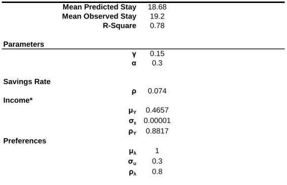
percentage of variation explained by the model is as close as possible to the total varia-tion. The percentage of explained variations by the model is 78 percent. The calibration

results predict in a mean stay of 18.86 years, compared to a observed mean stay of 19.2.

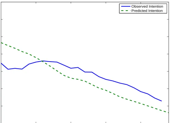
Figure 2.7 compares the observed intention of stay with the predicted one from our model. Predicted intentions refer to the average individual observed in our data

(who is 35 years old and has stayed already 15 years in Germany in 1984). Observed intentions refer to the intentions of those individuals with same age and years of

res-idence in Germany (plus minus two years) observed in the data. Migrants that stay in Germany revise their expected intentions upwards during their migration period. The

model captures fairly well this updating of expectations observed in the data.

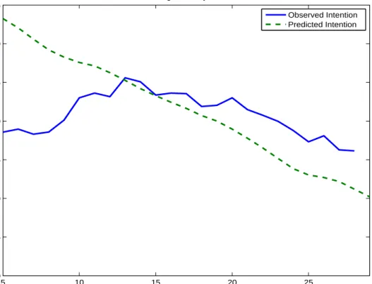
Figure 2.8 and Figure 2.9 perform a similar comparison between predicted and observed intentions for younger individuals with shorter stays and older individuals

with longer stays. Figure 2.8 shows the intentions of individuals aged 25 and that have stayed only 5 years in Germany in 1984. For those younger individuals with shorter

stays, the model does not predict as accurately the observed intentions, in particular on the first years of residence in Germany. For older individuals with longer stays, the

model does seem to predict pretty closely the observed intentions in the data (see figure 2.9).

The predicted intentions obtained using the calibration exercise are sensitive to

the parameters chosen to different degrees. On the one hand, predicted intentions are not very sensitive to the chosen savings rate parameterρ or to the relative income

pa-rameters (to a smaller extent). On the other hand, preference papa-rameters do modify significantly the predicted intentions in the calibration. A higher average relative

pref-erence for staying in Germany µλ reduces the probability of return and increases the

duration of stay in the host country. In addition, the results are sensitive to the relative

weight ofα and γ. Those combinations of parameters where α has a higher relative weight thanγ (like for the chosen calibrated parameters) have a much higher

explana-An alternative would be to use the actual individual income of the individual in the host country, which would take into account specific income shocks occurring to them.

(27)

2.5. Policy Analysis 27

tory power than the opposite.

2.5

Policy Analysis

The construction and calibration of the dynamic model allows to study the effect of

dif-ferent policies on migrant return intentions, our main objective. This section develops different policy scenarios and the effects they have on migrant intentions following the

model developed earlier.

The first policy simulation consists on a policy that gives a subsidy to those indi-viduals who return to their home country6_{. The subsidy should induce those}

individu-als who want to return to anticipate their return. The real effect should be to help those migrants who want to return but have not reach yet their savings target in Germany.

The effects of giving a subsidy equivalent to the income earned during half a year and during one year are shown in Figure 2.10. As in the previous section, the intentions

correspond to the average individual observed in our data in terms of age and length of residence in Germany. The figure shows that the effect of a subsidy modifies only

slightly the intentions to return of migrants at any point of their migration. On average, a subsidy equivalent to the income earned during half a year induces the individual to

reduce their intended stay in Germany by 100 days. A subsidy equivalent to one year income will induce a reduction on their intended stay of 208 days. In both cases, and

at different durations of stay, migrants only reduce slightly their intended stay in Ger-many. Thus only those migrants that were intending to return in the very near future

will anticipate their return, and the impact of such the policy will be very limited.

The second policy simulation corresponds to the impact of a change in the

eco-nomic conditions in the home country. A 20 % increase in the relative income of the home country increases the probability of return to the home country and reduces

the intended duration of stay in Germany (see Figure 2.11). The increase in relative income shown is equivalent to the increase in Spanish gdp per capita with respect to

the German gdp observed from 1984 to 2007, the period of study of the data 7. On average, the model predicts that the average migrant will reduce their intended stay by

6_{The subsidy could be offered either by the host country or by the home country.}

7_{During this period, the Spanish gdp per capita converged from 74.2% to 88.1% of the German gdp}

(28)

2.6. Conclusions 28

980 days (over two and a half years). The effect is heterogenous along the migration experience, being much larger at younger age and shorter stays. A migrant aged 35

and who stayed 15 years in Germany will reduce his intentions to stay in Germany by 1237 days (almost three and a half years shorter intended stay). At older age and longer

residence in Germany, the intentions however are almost unchanged.

Not only the average economic conditions of the home country, but also its

eco-nomic stability affects migrants intentions. Figure 2.12 compares the effect of home country economic conditions in our model between an average of all home countries

in the data versus Turkey’s economic conditions during the period studied. During that period, Turkey has a lower mean income, lower persistence and higher income

volatility 8. A Turkish migrant will have a longer intended stay in Germany than the average migrant due to the different economic conditions in his home country. This

difference in intended duration of stay in Germany is reduced the closer the migrant is to retirement age.

2.6

Conclusions

This study has developed a dynamic model to explain migrants’ plans to return to their

home country and how those are updated during the migration experience.

The policy simulations shown in the previous section have highlighted the

dif-ferent impacts that difdif-ferent policies and changes in the economic conditions of home countries can have in migrant return intentions.

Many countries have developed assisted voluntary return programs to incentivate

migrants to return to their home countries. However, those programs have had only moderate success (OECD (2008)). The policy simulations performed in this chapter

help explaining the small take-up rate of these return programs. The monetary subsidy offered is not sufficient to reduce migrants’ intended stay in the host country to a level

on which their return will be immediate. As migrants’ intentions are only reduced slightly, subsidy programs have only a limited effect on anticipating actual returns.

The policy simulations using our model show as well that an important aspect

mi-8_{More precisely, Turkish relative gdp during the period observed, modeled as AR(1), is equal to}

(29)

2.6. Conclusions 29

grants take into account are the economic conditions of the home country. Migrants’ in-tentions to return to their home country are substantially increased when the economic

conditions of their home countries improve. Migrants are more likely to consider an early return to their home country when it can offer them economic prosperity. If not,

they might not consider to return there, or at least not until retirement age.

This first chapter has considered the formation of migrants’ intentions to stay in

the host country and how they might be altered. The next two chapters will analyze the effect of changes in migrant’s intentions to stay in the host country on migrant’s

be-haviour there. In particular, chapter 3 will analyze the effect of intentions on remitting behaviour and chapter 4 on saving and asset holding behaviour.

(30)

Graph 1: Inflows and outflows of migrants in Germany by selected countries of origin, 1968-2008

Note: Statistisches Bundesamt, 1968-2008. Yugoslavia includes from 1992 to 2008 all the countries that previously formed Yugoslavia.

Turkey 0 50000 100000 150000 200000 250000 300000 1968 1972 1976 1980 1984 1988 1992 1996 2000 2004 2008 Inflows Outflows Yugoslavia 0 50000 100000 150000 200000 250000 300000 350000 400000 450000 1968 1972 1976 1980 1984 1988 1992 1996 2000 2004 2008 Inflows Outflows Italy 0 50000 100000 150000 200000 250000 1968 1972 1976 1980 1984 1988 1992 1996 2000 2004 2008 Inflows Outflows Greece 0 20000 40000 60000 80000 100000 1968 1972 1976 1980 1984 1988 1992 1996 2000 2004 2008 Inflows Outflows Spain 0 10000 20000 30000 40000 50000 60000 70000 1968 1972 1976 1980 1984 1988 1992 1996 2000 2004 2008 Inflows Outflows

Figure 2.1: Inflows and outflows of migrants in Germany by selected countries of ori-gin, 1968-2008

(31)

Mean St.Dev. Mean St.Dev. Mean St.Dev.

Age 35.2 13.0 41.3 12.9 45.7 11.0

Age at arrival 22.0 10.7 20.2 10.0 17.4 9.0

Years since migration 13.1 5.6 21.1 8.6 28.3 9.9

Year of arrival in Germany 1970.9 5.6 1974.9 8.6 1978.7 9.9

Intention to return (1=Yes; 0=No) 71.5% 45.1% 51.3% 50.0% 37.5% 48.5%

Intended stay duration (years) 18.1 16.5 20.6 14.0 18.7 11.2

Actual return (1=Yes; 0=No) 24.8% 43.2% 14.1% 34.8% 0.9% 9.5% Country of origin: Turkey 36.7% 48.2% 42.6% 49.5% 49.1% 50.0% Yugoslavia 18.5% 38.8% 23.2% 42.2% 23.3% 42.3% Italy 18.4% 38.7% 16.4% 37.1% 16.4% 37.0% Greece 14.0% 34.7% 11.7% 32.2% 7.7% 26.7% Spain 12.5% 33.1% 6.1% 23.9% 3.5% 18.4% Number Observations

Table 1. Descriptive Statistics

1984 1996 2007

Note: GSOEP, 1984-2007.

2946 1468 660

Table 2.1: Summary Statistics

(32)

Table 2: Variations in return plans Intention to Return in t Intention to Return in t-1 No Yes Total Yes 2753 12135 14888 % 18.49 81.51 100 No 7991 2568 10559 % 75.68 24.32 100 Total 10744 14703 25447 42.22 57.78 100 Note: GSOEP, 1984-2007.

Table 2.2: Variations in return plans

(33)

Graph 2: Changes in return intentions (difference in years)

Note: GSOEP, 1984-2007.

Figure 2.2: Changes in return intentions (difference in years)

(34)

Graph 4: Intentions of migrants over time

Note: GSOEP, 1984-2007.

Figure 2.3: Intentions of migrants over time

(35)

Table 3: Differences between intention to return in 1984 and actual return (prior to 2007)

Year of return No Yes Total

No return 654 1,353 2,007 1985 19 137 156 1986 5 47 52 1987 8 43 51 1988 12 55 67 1989 3 37 40 1990 10 24 34 1991 5 19 24 1992 11 13 24 1993 2 23 25 1994 7 29 36 1995 3 22 25 1996 6 21 27 1997 4 14 18 1998 5 15 20 1999 0 15 15 2000 1 12 13 2001 5 13 18 2002 0 8 8 2003 1 8 9 2004 3 8 11 2005 1 7 8 2006 1 3 4 Total 766 1,926 2,692 Note: GSOEP, 1984-2007. Intention to Return in 1984

Table 2.3: Differences between intention to return in 1984 and actual return (prior to 2007)

(36)

Graph 3: Difference in years between intended and actual stay durations

Note: GSOEP, 1984-2007.

Figure 2.4: Difference in years between intended and actual stay durations

(37)

Note: GSOEP, 1984-2007. Intended number of years of stay in the host country before return. 0 2 4 6 8 1 0 P e rc e n ta g e 0 10 20 30 40 50

Intended Years of Stay

Figure 2.5: Distribution of Migration Intentions

(38)

Note: GSOEP, 1984-2007. Intended number of years of stay in the host country before return. 0 1 0 2 0 3 0 0 1 0 2 0 3 0 0 10 20 30 40 50 0 10 20 30 40 50

0 to 9 Years Since Migration 10 to 19 Years Since Migration

20 to 29 Years Since Migration 30 or more Years Since Migration

P e rc e n ta g e

Intended Years of Stay

Graphs by ysmcat

Figure 2.6: Distribution of Migration Intentions by Duration of Stay

(39)

Table 4: Calibrated coefficients

Mean Predicted Stay 18.68 Mean Observed Stay 19.2

R-Square 0.78 Parameters γ 0.15 α 0.3 Savings Rate ρ 0.074 Income* µY 0.4657 σε 0.00001 ρY 0.8817 Preferences µλ 1 σu 0.3 ρλ 0.8

Observed savings rate during the period equal to 7.4% - see Table 4.2, chapter 2. * Income coefficients: coefficients from an estimated AR(1) process of the relative gdp between home and host country (1984-2007).

Rest of coefficients chosen such that predicted stay as close as possible to observed stay.

Table 2.4: Calibrated coefficients

(40)

Graph 5: Observed Intention vs. Predicted Intention

Note: GSOEP, 1984-2007.

Predicted intentions of an individual aged 35 and who stayed in Germany for 15 years in 1984. Average observed intentions of individuals aged 35 (+/- 2 years) and who stayed 15 (+/- 2 years) years in 1984. N=192 in 1985, N=47 in 2006. 15 20 25 30 35 0 5 10 15 20 25 30 35

Years Since Migration

Expected Intention till Return

Individual aged 35, 15 ysm in 1984

Observed Intention Predicted Intention

Figure 2.7: Observed Intention vs. Predicted Intention - Individual Aged 35 and 15 Years Since Migration

(41)

Graph 5b: Observed Intention vs. Predicted Intention - 25th

Note: GSOEP, 1984-2007.

Predicted intentions of an individual with 25th percentile characteristics, that is, aged 25 and who stayed in Germany for 5 years in 1984. Average observed intentions of individuals aged 25 (+/- 2 years) and who stayed 5 (+/- 2 years) years in 1984. N=91 in 1984, N=14 in 2006. 5 10 15 20 25 0 5 10 15 20 25 30 35

(42)

Graph 5c: Observed Intention vs. Predicted Intention - 75th

Note: GSOEP, 1984-2007.

Predicted intentions of an individual with 75th percentile characteristics, that is, aged 45 and who stayed in Germany for 25 years in 1984. Average observed intentions of individuals aged 45 (+/- 2 years) and who stayed 25 (+/- 2 years) years in 1984. N=138 in 1984, N=7 in 2006. 15 20 25 30 35 0 5 10 15 20 25 30 35

(43)

Graph 5: Effect of subsidy to return to home country

Note: GSOEP, 1984-2007. Calibrated coefficients (table 2.4.). Individuals with average age (35) and years since migration (15) in 1984.

15 20 25 30 35 40 0 0.1 0.2 0.3 0.4 0.5 0.6 0.7 0.8 0.9 1

Probability

Without Subsidy

With Half Year Income Subsidy With One Year Income Subsidy

15 20 25 30 35 40 0 5 10 15 20 25

Intended Duration of Stay

Figure 2.10: Effect of subsidy to return to home country

(44)

Graph 6: Effect of change in relative income

15 20 25 30 35 40 0 0.05 0.1 0.15 0.2 0.25 0.3 0.35 0.4 0.45 0.5

Probability

No Change

20% Increase Relative Income

15 20 25 30 35 40 0 5 10 15 20 25

Figure 2.11: Effect of change in relative income

(45)

Average economic conditions in home country versus Turkey's economic conditions during 1984 - 2007 (lower mean income, lower persistence and higher income volatility).

Graph 7: Effect of different home country economic conditions: average versus Turkish economic conditions (lower mean income, lower persistence and higher income volatility) 15 20 25 30 35 40 0 0.05 0.1 0.15 0.2 0.25 0.3 0.35 0.4 0.45 0.5

Probability

Average Y Home Country

Turkish Y:lower mu, lower rho, higher sigma

15 20 25 30 35 40 0 5 10 15 20 25 30

Figure 2.12: Effect of different home country economic conditions

(46)

Chapter 3

Remittances and Temporary

Migration

∗

∗_{This chapter has been co-authored with Christian Dustmann and has been published in}_{Journal of}

Development Economics, Volume 92, pages 62-70, 2010. We are grateful to two anonymous referees

(47)

3.1

Introduction

The amount of remittances sent by immigrants back to their home countries has

in-creased steadily over the last decades. Currently, the volume of remittances to devel-oping countries using formal channels is estimated to be over $240 billion (Ratha et al.

(2007)). Their level is higher than official development aid and close to foreign di-rect investment and other capital inflows for developing countries. Remittances help

economic development and are a major factor in poverty reduction1. In addition, re-mittances are now one of the primary sources of foreign exchange for many receiving

countries.

For immigration countries, remittances constitute a non-negligible outflow of cap-ital. Recent figures suggest that the outflow of remittances from high income OECD

countries is over $136 billion (Ratha et al. (2007)). For instance, in Germany the vol-ume of remittances was about 0.31% of GDP in 2003 (Bundesbank (2008)).2 _This

was equivalent to 150 % of Germany’s total budget for official development aid in that year3_.

It is therefore not surprising that a large literature has developed on the subject,

see Docquier & Rapoport (2006) for an excellent survey. Key issues to understand are which migrant populations remit, for which purpose, and what determines the amount

of remittances. Answers to these questions may help to create migration schemes that affect the way remittances are channeled into different purposes, thus supporting their

optimal efficiency for economic development, and raising awareness about how differ-ent policies will lead to differdiffer-ent incdiffer-entives to remit.

A number of papers develop models for the different motives that may trigger

remittances, and explore some of their empirical implications.4 This research has pro-vided us with a wealth of insight. Yet, on the empirical level we still know relatively

1_{See e.g. Adams (2006}_a_{), Adams (2006}_b_{) and Acosta et al. (2006) for analysis.}

2_{Germany is the third largest source country of remittances payments, after United States and Saudi}

Arabia, see Ratha (2003).

3_{Official Development Assistance accounted for 0.21% of GDP in Germany in 2003, see OECD}

(2005).

4_{See e.g. Lucas & Stark (1985), Lucas & Stark (1988), Hoddinott (1994), Funkhouser (1995), Poirine}

(1997), Agarwal & Horowitz (2002), de la Briere et al. (2002), Faini (2006), Okonkwo Osili (2007), Amuedo-Dorantes & Pozo (2006) and Hanson (2007).

(48)

3.2. Remittances and return migration 48

little about the determinants of remittances, the various forms remittances may take, and how these interact with migrant behavior and the forms of migration. One

partic-ular aspect, which is in our view important, is the way the permanency of a migration affects the magnitude and purpose of remittance flows.

We address these questions in this paper. We analyze how remittance flows are

related to the permanency of migration, and to the residential location of the family. Our empirical analysis is based on a panel data set of immigrants over the period from

1984-1994. This data contains repeated information about whether, and what amount of remittances is sent. It also distinguishes between remittances for family support,

savings, and for a residual category ”other purposes”. Due to the information our data provides us about the return plans of immigrants, we are able to distinguish between

in-dividuals who consider their migration as temporary, and who consider their migration as permanent. The panel nature of our data, and repeated information on remittances

as well as return intentions, allows us to explore and isolate the way the permanence of migration, as well as the locational distribution of the family, affect remittance flows,

conditional on observed characteristics and unobserved fixed differences across house-holds in their remittance propensity. We address measurement error problems and

pos-sible feedback of past remittances on current return plans by combining a fixed effects

estimator with an IV strategy.

The structure of the paper is as follows: in section 2 we discuss the way remit-tances may be affected by return plans, and introduce our estimation strategy. In

sec-tion 3 we provide some background informasec-tion and discuss the data and our sample. In section 4 we show our estimation results, and section 5 concludes.

3.2

Remittances and return migration

A difficulty with remittances is its measurement and exact definition. If we define re-mittances as all transfers from the immigration country to the immigrant’s home

coun-try (a definition which we will follow below), then remittance flows consist of both transfers to support family and kinship in the origin country, as well as savings or

in-vestments for future consumption at home. The motivation for both types of transfers is different. While the first requires altruistic behavior and/or influence through the

(49)

Dustmann (1997)).

Transfers for both family support and savings purposes may differ according to

whether the migration is considered as temporary or as permanent. Remittances to sup-port family and kinship can be viewed as intra-family transfers across national borders.5

Thus, if temporary migrants have more of their (extended) family living abroad, they may remit more. Further, remittances may also respond to expectations about

fulfill-ment of family and social commitfulfill-ments. Satisfying these expectations can be seen as a price to be paid for the option to return back home at a later stage, or as an ”insurance”

to be welcomed in the home community after returning. Also this motive would result in higher remittances of temporary migrants.6

Remittance flows may further be motivated by the wish to hold assets or savings

in the home country. These may take the form of housing stock, capital investments, or simply savings. Thus, remittances motivated in this way are not different from an

intertemporal allocation of consumption, or investment into durable consumption goods across national borders.7 _{A positive probability of return may affect these transactions}

either by inducing a preference to holding assets and savings in the home country, or by inducing immigrants to shift more consumption from the present to the future, or

both.

3.2.1

Empirical specification

Our main interest is in determining how the level of remittances is affected by house-hold characteristics, and by immigrants’ return plans. We estimate regressions of the

following type:

Yit =a0+a1Xit+ξRit+i+uit, (3.1)

where Yit measures remittances, and the indices i and t denote households and

5_{See Lucas & Stark (1985) for an early discussion. See Cox (1987), Cox et al. (1998) for empirical}

analysis of altruistic motives for private transfers. For a recent survey on the private transfer literature see Laferrere & Wolff (2000).

6_{Azam & Gubert (2006) stresses the role of the extended family and the village in migration and}

remittance decisions. Amuedo-Dorantes & Pozo (2006) investigates this motive empirically.

7_{As Durand et al. (1996) recognizes, ”sending monthly remittances (...) and returning home with}

savings are interrelated behaviors that represent different ways of accomplishing the same thing: repa-triating earnings”.

(50)

time. The key variable of interest isRit, which is a measure of the temporariness of

the migration. As we explain below in more detail, we obtain this variable from survey

questions on the migrant’s intention to return home, which we observe in every wave of the panel that we use. These intentions may change over the migration history, and

they may not always correspond to whether the migration has finally been permanent. But it is exactly theseplansabout a future return that determine remittance behavior.

The vectorXitcollects characteristics of the household and the head of household.

We include here the log of disposable household income, the number of adults and the

number of children (below the age of 16) living in the household, and the number of employed household members. We also include characteristics of the head of

house-hold, like the gender, the employment status, the years since migration and its square, the number of years of education, and whether the partner is native born or the

house-hold head is single. Further, we include variables about whether the spouse or children are living abroad, and an indicator variable whether the head of household grew up in

a rural area.

3.2.2

Identification

There are a number of problems with the estimation of equation (3.1). First, individu-als who tend to return may at the same time have a higher (lower) propensity to send

remittances. In this case, our estimate ofξ will be possibly upward (downward) bi-ased, as the individual effect i will be correlated with return intentions Rit, so that

E(i|X, R) 6= 0.8 Some of this bias is likely to be eliminated by conditioning on the

variables inX.

A further problem is that return intentions are likely to be measured with (possi-bly considerable) measurement error, thus creating an attenuation bias. In this case the

”observed” return intention equals R∗_it = Rit +Mit. We assume here that the

mea-surement errorMit has the ”classical” properties of being uncorrelated with the true

intention and being serially uncorrelated (E(Rit, Mit) = 0, E(Mit, Mis) = 0, t 6= s).

The downward bias is greatly exacerbated when estimating the model in differences or

using fixed effects (see e.g. Hsiao (1986) for a detailed discussion).

8_{If on the other hand, these individuals tend to save more in the host country rather than to remit,}

(51)

Finally, remittances in previous periods may affect later return plans. For instance, past remittances, invested into assets or durable consumption goods, may have created

returns that lead immigrants to change their current return intentions. This would imply that Rit =b0+b1Xit+ t−1 X s=1 dsYis+φ i+vit. (3.2)

If a positive shock to past remittances positively affects present return plans (ds>

0), then this would lead to a downward bias when using a difference or a fixed effects estimator. We deal with these problems by combining a fixed effect type estimation strategy (using within household variation for estimation only) with an instrumental

variable estimator. The idea of our estimation strategy is as follows. In a first step, we eliminate the fixed effects by using a ”forward orthogonal deviations” transformation

(Arellano (2003)). This transformation removes the fixed effects by subtracting from each observationt = 1, ..., T−1the mean of the remaining future observations (rather than the mean of all observations, as does the standard FE estimator) in the sample. The forward orthogonal deviations transformation of a variableXitis defined asXit0 = p

(T −1)/(T −t+ 1)(Xit− _T1₋₁PT_s₌_t₊₁Xis)(see Arellano (2003) a