R E S E A R C H A R T I C L E Open Access
Is there any gender gap in the production of legumes
in Malawi? Evidence from the Oaxaca
–
Blinder
decomposition model
Uzoamaka Joe-Nkamuke1 &Kehinde Oluseyi Olagunju2&
Esther Njuguna-Mungai3&Kai Mausch4
Received: 22 July 2018 / Accepted: 9 September 2019/ #The Author(s) 2019
Abstract
Understanding the gender differences in agricultural productivity is crucial for formu-lating informed and effective policies to sustainably improve low productivity which characterises agriculture in Sub-Sahara Africa. Using a panel dataset from the ICRISAT
led Tropical Legumes project III (2008–2013), we analyse the gender gap in the
production of legumes in Malawi. Employing the Oaxaca–Blinder decomposition
method allows decomposition of gender gap into the following: (i) the portion caused by observable differences in the factors of production (endowment effect) and (ii) the unexplained portion caused by differences in return to the same observed factors of production (structural effect). We conducted the empirical analysis separately for pigeonpea and groundnut. Our findings reveal that for groundnut cultivated plots, women are 28% less productive than men after controlling for observed factors of production; however, the gender gap estimated in the pigeonpea cultivated plots are not statistically significant. The decomposition estimates reveal that the endowment effect is more relevant than the structural effect, suggesting that access to productive inputs contributes largest to the gender gap in groundnut productivity, and if women involved had access to equal level of inputs, the gap will be reduced significantly. The variation in the findings for groundnut and pigeon plot suggests that policy orientation towards reducing gender productivity gap should be crop specific.
Keywords Agricultural productivity . Gender differences . Decomposition . Malawi
Introduction
Low productivity characterises the agricultural sector in sub-Saharan African (SSA) which informs major agricultural intervention programmes in this region focusing on
https://doi.org/10.1007/s41130-019-00090-y
* Uzoamaka Joe-Nkamuke uzosecond@gmail.com
changing the prevailing circumstance. The barriers female farm managers' face resulting in their reduced productivity compared to their male counterparts can be said to be a major contributor to low productivity in the region. Despite high-priority roles that women play in SSA agriculture, accounting for approximately 50% of the agri-cultural labour force involved in all levels and types of agriagri-cultural activities, several empirical studies have identified that female farmers are disadvantaged in production process and have lower yields than their male counterparts, thereby creating a produc-tivity gap that ranges from 20 to 30% and, as such, further mitigating agricultural
productivity potential in SSA.1According to the report of the Food and Agriculture
Organization in2011and the World Bank in2014, productivity potentials of African
women in agriculture are constrained in several ways. First, from a political and socio-cultural point of view, women perhaps have unequal access to farmland compared with men, and in case they do, they are weakened by land tenure security (Arturo et al.
2015). Another reason is that female farmers have limited channels through which they
can access productive inputs; for instance, their access to improved varieties and agricultural extension services are less compared with that of their male counterparts subjecting them to inadequate use of fertilisers, labour, seeds and other inputs needed
for optimal production. Also, women membership in farmers’ organisation, such as
labour-saving cooperatives, producers’organisation and marketing group, is limited,
thereby curtailing their access to product markets and more importantly, resource allocation potential. Finally, the gender gap in productivity, at the disadvantage of
women, may also be adduced to women’s dual commitments as farm managers and
household managers constraining their allocative efficiency which becomes more severe with low levels of their education, when compared with their male counterparts. A reasonably genuine attempt to raise agricultural productivity in SSA is therefore contingent upon effectively reducing and or eliminating the productivity gap which exists between male and female farmers. Food and Agricultural Organization asserts in their report in 2011 that developing countries of the world have the potential of
increasing their aggregate agricultural output by 2.5–4.0% provided that they are able
to reduce productivity gap between male and female farmers to its least minimum. Studies on the factors explaining productivity differences between male and female
farmers across SSA are well established in the literature. For example, Kilic et al. (2015)
find that female plot managers in Malawi devote less time to productive activities, as a result of high child dependency ratio, resulting to being about 25% less productive compared with their male counterparts. A similar investigation was carried out by
Gbemisola et al. (2015) who further empirically establish the gender productivity gap
in Nigeria by region. In the Northern region of Nigeria, women are 28% less productive with a large proportion of the gap attributed to structural/unexplained effect, while no significant gender productivity differences in the Southern part of the country. Notably
from the findings of Gbemisola et al. (2015), the gender gap in productivity within a
country may differ across different regions in the country. In another empirical study
conducted by Ali et al. (2016), the difference in the yield between male and female
cultivated plots was estimated to be 17.5%, also to the disadvantage of female managers in Uganda largely attributed to difficulty in accessing productive inputs, negligible
households endowments, ‘double-edged’ childcare and farming responsibilities, and
1
difficulty in accessing output markets. Nonetheless, all these early empirical studies are limited by the methodological approach, geographical data coverage and little attention given to the specificity of different farming enterprises. Gender gap estimates differ with different geographical locations and farming enterprises, perhaps because of different socio-economic needs and agro-economic and environmental challenges, amongst other
factors (Gbemisola et al. 2015). Therefore, generalising gender gap of productivity
differences may not be appropriate for informed and effective sub-sectoral agricultural
and gender policies. To our knowledge, only Gbemisola et al. (2015) have been able to
empirically validate the gender gap in agricultural productivity by region in Nigeria; however, the study did not extend its investigation to different farming enterprises; therefore, recommendations from this study may only be applicable to regional produc-tivity and gender policies but not sub-sectoral policies.
Our article contributes to the existing debate on the gender gap in productivity by providing evidence for productivity gap not only at the national level but also for farmers that produce two major crop legumes in Malawi, thereby proffering a better understanding of gender gap by farming enterprise. Also, we take advantage of our household panel dataset to explore the most appropriate unit of analysis for this present
study—the individual plot—while also controlling for other characteristics of the plot
manager with other explanatory variables. According to Doss (2001), the use of sex of
household head as gender indicator is problematic as it does not reflect the actual economic unit that makes decisions in respect to what to cultivate, with an unclear assumption that production decision within the household is solely taken by the household head. Our study differs from this unclear assumption as we base our definition of gender indicator on the notion that production decisions are mainly taken by the plot manager; therefore, we employ gender of plot managers, instead of the gender of the household head, as the gender indicator. The use of gender of plot
manager was adopted by Gbemisola et al. (2015), Kilic et al. (2015) and Arturo et al.
(2015). Regarding the analytical approach, we go beyond providing insight on the
factors that explain productivity differences between male and female, conventional practice in existing studies, but also provide estimates of the relative contribution of these factors to productivity gaps between male and female-managed plots using the
Oaxaca–Blinder decomposition model. The use of the model allows us to partition the
mean difference in yield between male-managed plot and female-managed plot into two parts. The first part constitutes the portion that is driven by gender differences in levels of observable attributes (i.e. the endowment effect), and the second part consti-tutes the portion that is motivated by gender differences in return to the same set of
observables (i.e. the structure effect) (Jann2008). By doing this, we have been able to
provide estimates of the relative contribution of the different drivers of productivity differences between male and female groundnut and pigeonpea plot managers in Malawi. We are not aware of any previous study that applied this method to analyse the gender gap in the production of crop legumes in agriculture. Finally, this study is of importance to Malawian agricultural and gender policies considering the statistical joint
report of the UNEP and the World Bank (2015) which reveals that women farmers in
Malawi are older by over 5 years on average and also have lower levels of education as compared with male farmers, suggesting that Malawian women are approaching less economic active years with low social and human capital than men. With legumes
Njuki et al. 2011), we explore two major leguminous crops in Malawi, namely, groundnuts and pigeonpea, and by doing this, we have been able to provide a better understanding of gender gap in productivity analyses with respect to crop specificity and farm decision-making.
The presentation of the remaining sections of the papers is as follows. The“
Pro-duction of legumes and gender issues in Malawi”section provides background on the
production of legumes and gender issues in Malawi, while the“Data and descriptive
statistics”section details the data utilised and the summary statistics of the variables
used in the empirical estimation. The“Methodology”section explains the methodology
used. The estimated results are reported and discussed in the “Empirical results”
section. We conclude in the“Conclusion”section.
Production of legumes and gender issues in Malawi
Agriculture remains a very important sector in the Malawian economy, accounting for about one-third of overall gross domestic product (GDP) in the year 2016 and 2017 (see
Fig.1). Its contribution to economic growth is immense in terms of employment, export
earning, livelihood support, food and nutrition security and gender equality. Poverty trends in the country are largely driven by poor productivity performance of the agricultural sector evidenced in the falling share of agriculture in the GDP. In Malawi, the majority of smallholder farmers have shifted to the cultivation of leguminous crops in the last 10 years. Groundnuts and pigeonpea are the most important crop legumes cultivated in the country.
Groundnut is the most important legume and oilseed crop in terms of total produc-tion and area under cultivaproduc-tion in Malawi. The average annual cultivated area for
groundnuts for the period 1991–2006 (171 thousand hectares) accounted for 27% of the
total legume land cultivated (ICRISAT2013). It thrives under low rainfall and poor
soil, hence requiring minimum capital investment (Hamidou et al.2013). Its multiple
uses make it a very important food and cash crop. In Malawi, similar to many SSA countries, groundnut is predominantly grown and managed by women and considered a
women’s crop (Naidu et al.1999; Orr et al.2015); its cultivation, therefore, has a direct
10 15 20 25 30 35 40 45 50 55 19 60 19 62 19 64 19 66 19 68 19 70 19 72 19 74 19 76 19 78 19 80 19 82 19 84 19 86 19 88 19 90 19 92 19 94 19 96 19 98 20 00 20 02 20 04 20 06 20 08 20 10 20 12 20 14 20 16 % o f GDP Year
effect on overall economic, financial and nutritional well-being of women and children
(Mbeiyererwa et al. 2012). Also, it is regarded as a valuable crop, contributing
tremendously to improving household food security, nutrition, soil health and fertility, while being an important source of cash income for smallholder farmers
(Chiyembekeza et al.1998) making up over 25% of their agricultural cash income
(Dorward and Chirwa2011). However, due to numerous constraints, its productivity
still remains low.
Another very important crop legumes in Malawi is pigeonpea; it is‘dubbed’welfare
crop for smallholder farmers because they can be intercropped with maize, sorghum or
groundnuts without significantly reducing their yields (Kanyama-Phiri et al. 2008).
They are also drought-resistant and like other legumes improve soil fertility through nitrogen fixation and decay of fallen leaves. As a source of protein in many African and Asian countries, its immature seeds and pods are consumed as green vegetables, its leaves, stems, husks and pod wall form quality animal feed and its dried stems are a
good source of fuel food (Simtowe et al.2009). Malawi remains one of the largest
producers of pigeonpea on the continent producing about 80,000 metric tonnes per
annum and exporting about 25% of its produce (Malawi Ministry of Agriculture2016).
In Malawi, similar to other SSA countries, women play significant roles in agricul-tural production and are exclusively involved in homemaking. Women labour partic-ipation in Malawian agriculture is slightly higher compared with some selected SSA
countries. For example, Palacios-Lopez et al. (2017) estimated the average female
labour share in crop production in Malawi to be 50%, higher than Nigeria (37%), Ethiopia (29%) and Niger (24%). This is suggestive of the importance of women in agricultural production in Malawi. A number of studies have argued that African women work longer hours than men, engaging in both domestic and economic activities. Malawian women are actively involved in agricultural value chain activities ranging from planting through to harvesting, processing and marketing. Unfortunately, they are mostly confined to work in small fields with less yield potential. This is mainly because they have limited access to productive resources compared with their male counterparts. This gap also exists in other socio-economic characteristics that affect agricultural productivity such as level of education and membership of cooperative groups. In the same vein, most African traditions, Malawi inclusive, coupled with the socio-cultural architect in most local communities restrict land rights to men, in most
cases, after marriage dissolution (Fafchamps and Quisumbing2002), which has further
widened productivity gap between men and women. Notably, in recent years, women participation in agricultural production has witnessed some changes as a result of changing sociopolitical and economic situations in most African countries (Saito
et al.1994). In response to this, the Malawian government has put together a national
gender policy in March 2015 which focuses on improving women’s access to soft and
hard infrastructure such as credit services, extension services, public markets and education. Similarly, the policy aims at promoting overall active participation of women in Malawian agricultural economy targeted at improving agricultural yield
and in particular cereal yield. As shown in Fig.2, cereal yield in Malawi has lagged
behind the world’s cereal yield in the last five decades. In spite of the implementation of
the policy, female is still by far less productive in Malawi (Kilic et al.2015). This may
likely in part be attributed to lack of farm enterprise specificity in the 2015 National Gender Policy. In this study, we provide up-to-date evidence of the gender gap in the
production of legumes in Malawi by analysing the factors that drive these differentials and provide policy recommendations that are specific to each of the two main cereal crops to bridge this gap.
Data and descriptive statistics
The empirical analysis of the study is based on a cross-section of data for three planting
seasons—2008, 2010 and 2013, from the Malawian national household surveys
con-ducted within the Tropical Legumes III (TL-III) project. The survey was concon-ducted in the two main agricultural regions in Malawi, namely, central and southern regions. Data was collected from the two regions and 4 districts within these regions. In the central region, data was collected from Mchinji district while in the Southern region data was collected from Balaka, Chiradzulu and Thyolo districts. Thyolo, Chiradzulu and Balaka are major pigeonpea-growing areas and grow groundnut moderately while Mchinji is a major groundnut-growing area. The information collected in the survey includes household and farmer characteristics, plot characteristics, inputs and outputs used, household asset ownership and knowledge of improved crop varieties. A total of 594, 439 and 208 households were surveyed in 2008, 2010 and 2013 respectively. Following data cleaning, we arrive at 582, 423 and 149 observations from the 3 time periods generating an unbalanced panel dataset.
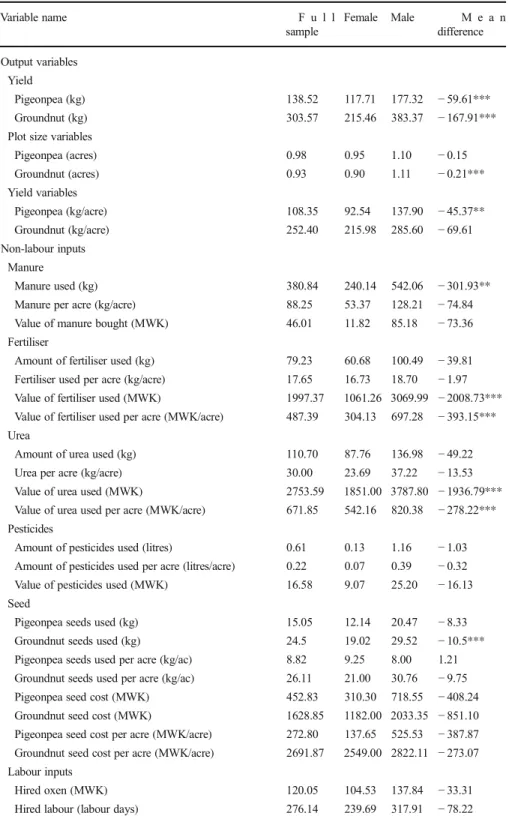
In Table 1, we present the summary statistics of all the variables used in the
empirical analysis which include the outcome variables (groundnut and pigeonpea yield), the relevant independent variables and the test of the mean difference between the male and female managers. The table provides the first foretaste of the gender gap that exists in the aggregate production and yield of both pigeonpea and groundnut, revealing that male managers have more aggregate production and are may be more productive than female managers. A similar gap is also observed in the plot size cultivated, with female-managed plots 14% and 19% less on average for both
pigeonpea and groundnut respectively than male cultivated plots. In Fig.3, we present
the kernel density plots of the log of the yield of pigeonpea and groundnut per acre of 200 700 1200 1700 2200 2700 3200 3700 4200 4700 19 61 19 63 19 65 19 67 19 69 19 71 19 73 19 75 19 77 19 79 19 81 19 83 19 85 19 87 19 89 19 91 19 93 19 95 19 97 19 99 20 01 20 03 20 05 20 07 20 09 20 11 20 13 20 15 20 17 Cereals y ield (Kg/h a) Year Malawi World
Table 1 Summary statistics for the full sample and by gender of the plot manager Variable name F u l l sample Female Male M e a n difference Output variables Yield Pigeonpea (kg) 138.52 117.71 177.32 −59.61*** Groundnut (kg) 303.57 215.46 383.37 −167.91*** Plot size variables
Pigeonpea (acres) 0.98 0.95 1.10 −0.15 Groundnut (acres) 0.93 0.90 1.11 −0.21*** Yield variables Pigeonpea (kg/acre) 108.35 92.54 137.90 −45.37** Groundnut (kg/acre) 252.40 215.98 285.60 −69.61 Non-labour inputs Manure Manure used (kg) 380.84 240.14 542.06 −301.93** Manure per acre (kg/acre) 88.25 53.37 128.21 −74.84 Value of manure bought (MWK) 46.01 11.82 85.18 −73.36 Fertiliser
Amount of fertiliser used (kg) 79.23 60.68 100.49 −39.81 Fertiliser used per acre (kg/acre) 17.65 16.73 18.70 −1.97 Value of fertiliser used (MWK) 1997.37 1061.26 3069.99 −2008.73*** Value of fertiliser used per acre (MWK/acre) 487.39 304.13 697.28 −393.15*** Urea
Amount of urea used (kg) 110.70 87.76 136.98 −49.22 Urea per acre (kg/acre) 30.00 23.69 37.22 −13.53 Value of urea used (MWK) 2753.59 1851.00 3787.80 −1936.79*** Value of urea used per acre (MWK/acre) 671.85 542.16 820.38 −278.22*** Pesticides
Amount of pesticides used (litres) 0.61 0.13 1.16 −1.03 Amount of pesticides used per acre (litres/acre) 0.22 0.07 0.39 −0.32 Value of pesticides used (MWK) 16.58 9.07 25.20 −16.13 Seed
Pigeonpea seeds used (kg) 15.05 12.14 20.47 −8.33 Groundnut seeds used (kg) 24.5 19.02 29.52 −10.5*** Pigeonpea seeds used per acre (kg/ac) 8.82 9.25 8.00 1.21 Groundnut seeds used per acre (kg/ac) 26.11 21.00 30.76 −9.75 Pigeonpea seed cost (MWK) 452.83 310.30 718.55 −408.24 Groundnut seed cost (MWK) 1628.85 1182.00 2033.35 −851.10 Pigeonpea seed cost per acre (MWK/acre) 272.80 137.65 525.53 −387.87 Groundnut seed cost per acre (MWK/acre) 2691.87 2549.00 2822.11 −273.07 Labour inputs
Hired oxen (MWK) 120.05 104.53 137.84 −33.31 Hired labour (labour days) 276.14 239.69 317.91 −78.22
male- and female-managed plot samples which also provide evidence of gender differences in the production of legumes. The average pigeonpea plot size managed by the female is 0.95 acre, while that of the male is 1.10 acre. In the case of groundnut, on average, males manage 1.11 acre while females manage 0.90 acre.
According to Gbemisola et al. (2015), differences in productivity between male- and
female-managed plots may in part be due to input use. In Table1, we observe a gender
Table 1 (continued)
Variable name F u l l
sample
Female Male M e a n difference Hired labour days per acre (labour days/acre) 64.46 56.70 73.36 −16.66 Labour (labour days/acre) 20.91 15.25 27.98 −12.73** Family labour days per acre (labour days/acre) 4.42 3.71 5.31 −1.60 Manager characteristics
Age (years) 44.16 44.71 43.54 1.17 Education (years) 4.45 3.76 5.17 −1.41*** Number of months on the farm in the last 12 months
(months)
9.64 9.62 9.66 −0.04 Number of years in village (years) 33.05 35.98 29.7 6.28*** Groundnut experience (years) 9.88 10.04 9.69 0.35 Pigeonpea experience (years) 14.76 16.29 12.28 4.01*** Responsibility in the community (1 = yes, 0 = otherwise) 0.26 0.18 0.37 −0.18*** Divorced (1 = yes, 0 = otherwise) 0.09 0.15 0.02 0.13*** Married (1 = yes, 0 = otherwise) 0.75 0.61 0.92 −0.31*** Never married (1 = yes, 0 = otherwise) 0.02 0.01 0.02 −0.01 Widow/widower (1 = yes, 0 = otherwise) 0.13 0.22 0.03 0.09*** Household head (1 = yes, 0 = otherwise) 0.70 0.46 0.97 −0.52*** Spouse of household head (1 = yes, 0 = otherwise) 0.29 0.52 0.01 0.51*** Casual labourer on the farm (1 = yes, 0 = otherwise) 0.01 0.03 0.02 −0.01** Main occupation
Farming (1 = yes, 0 = otherwise) 0.95 0.97 0.92 0.05*** Off-farm salaried-employment (1 = yes, 0 = otherwise) 0.02 0.01 0.03 −0.02** Off-farm self-employed (1 = yes, 0 = otherwise) 0.01 0.01 0.02 −0.01 Farm labour participation
Full time worker (1 = yes, 0 = otherwise) 0.94 0.96 0.92 0.04*** Not a worker (1 = yes, 0 = otherwise) 0.01 0.01 0.00 0.01 Part-time worker 0.05 0.03 0.07 −0.04** Plot ownership
Borrowed (1 = yes, 0 = otherwise) 0.02 0.01 0.02 −0.01 Owned (1 = yes, 0 = otherwise) 0.88 0.87 0.89 −0.02 Rented (1 = yes, 0 = otherwise) 0.10 0.11 0.09 0.02
Observations 1154 618 536
Notes: Significant mean differences are indicated with ***p< 0.01, **p< 0.05, *p< 0.1; MWK is Malawian kwacha (1000 MWK = 1.35USD)
gap in the use of labour and labour productive inputs. The quantities of all non-labour productive inputs used by male managers are larger than the female managers. Specifically, female managers use 56% less than the average quantity of manure used by the male managers, but the difference becomes insignificant after normalising for plot size. The value of fertiliser used by female managers is 65% less than that used by male managers and even when normalized by plot size, female managers still use 56% less than male managers per acre of land. Value of urea used by female managers is 32% less than the average of the pooled sample and 51% less than that used by male managers. Surprisingly, we do not observe any significant difference in the quantity of pigeonpea seeds used between the male and female manager, but we find a significant difference in the groundnuts seeds used between male and female managers. Male managers use 29.5 kg (36%) more groundnuts seeds than female managers (19.02 kg) but this difference becomes insignificant after normalising seeds used by plot size. As
for labour inputs, Table1 shows that male-managed plots use more hired and family
labour than their female counterparts although the differences are not significant for all the labour input variables except for family labour days when we normalise by plot size.
Turning to the characteristics of the plot managers, female managers are slightly older than male managers; spend less time on the farm, since some of them largely engaged in processing and marketing compared with male managers. The male man-agers attain more years of schooling than female manman-agers. This difference is quite significant which is in line with the 2015 United Nations report. Also, female managers have spent years more on average in the village, have more years of farming experience with pigeonpea than their male counterparts and are assigned fewer responsibilities in their communities. There are more divorced and less married female plot managers since most of the female managers are widowed. Unsurprisingly, in line with African tradition, female managers are less likely to be household heads and participate less in off-farm employment compared with male managers. Finally, female managers partic-ipate lesser in land markets in terms of renting, borrowing and land ownership.
Methodology
OLS estimation with fixed effect
Following the canonical approach in the literature for examining the existence and magnitude of the gender gap in productivity, we construct a yield function framework which models the quantity of output per acre as a function of the gender of the plot
manager and other factors that affect production.2We employ this approach because it
can be used to determine if any other factors can explain the gender productivity gap other than the gender indicator. In deciding the gender indicator, we explore the provision from our dataset that contains the gender of the plot manager rather than the gender of the household head who may have less decision-making influence on the
2
The framework assumes a Cobb–Douglas constant return to the scale production function in which the dependent and the input variables per unit of land can be transformed into logarithmic forms (Barrett et al.
plot. Conventionally, a simple yield function according to Udry et al. (1995) is
presented in Eq. (1) below.
Yab¼θþβGabþαZabþδbþμab; ð1Þ
whereYabis the natural logarithm of value of yield of plotaunder managerb;θis the
unknown constant;Gab is a dummy variable capturing the gender of the manager of
plota;Zabcontains vectors of covariates other than gender including the plot manager’s
characteristics (age, education, marital status), plot characteristics (distance to market, waterlogging on plot), cropping strategies (irrigation, use of improved seeds) and set of labour and non-labour inputs used on the plot (hired oxen, hired labour, seeds,
fertilisers, manure);δb is a fixed effect that captures all time-invariant characteristics
of the managerb; andμabis the stochastic error term. In recent empirical studies, the
model is extended to include longitudinal data and fixed effects. The specification in
Eq. (1) is for cross-sectional dataset. The use of panel data helps to control for
unobserved heterogeneity. Based on the aforementioned and our panel dataset, we
estimate Eq. (2).
Yabt¼βGabtþαZabtþδbþωetþμabt; ð2Þ
whereYabtis the natural logarithm of value of yield of plotaunder managerbduring
seasont;Gabtis a dummy variable capturing the gender of the manager of plotaduring
seasont;Zabt contains vectors of covariates other than gender for plota in seasont
which includes the plot manager’s characteristics (age, education, marital status), plot
characteristics (distance to market, waterlogging on plot), cropping strategies (irriga-tion, use of improved seeds) and set of labour and non-labour inputs used on the plot
(hired oxen, hired labour, seeds, fertilisers, manure);δbis a fixed effect that captures all
time-invariant characteristics of the managerb; ωet is a fixed effect that captures all
time-variant characteristics of the regionsein seasont; andμabtis the stochastic error
term. In the analysis, we include the season (time) fixed effect to account for season-specific error that may arise from the systemic shock.
(a) (b) 0 .1 .2 .3 yti s n e D 0 2 4 6 8
Female managers Male managers
0 .1 .2 .3 .4 0 2 4 6 8
Female managers Male managers
Fig. 3 Kernel density plots of the log of the yield of pigeonpea (a) and groundnut (b) per acre of male- and
The purpose of the model in Eq. (2) is to test the hypothesis that yield of the plots that are managed by the female is not significantly different from the yield of the plots
that are managed by the male (β= 0).
Our estimation is in six steps using a progressive approach. The first step (naïve regression) considers only the gender of the plot manager as only the independent variable. In the next steps, more control variables are included. The characteristics of the plot managers are included in the second step, plot characteristics and plot size in the third step, cropping strategies adopted in the fourth step, labour inputs used in the fifth step and non-labour inputs used in the sixth which is the final step. We decided to
run our analysis in this way, following Gbemisola et al. (2015), with the motivation that
the approach is able to answer the question of ‘if’ and ‘how’ each of the set of
covariates affects the gender productivity gap.
Oaxaca–Blinder decomposition approach
The OLS-fixed effect analysis presented in the previous section is able to examine the factors that influence productivity gap that exists between the plots managed by male and those by the female; however, the approach does not help us understand the relative contribution of these factors to the productivity gap. To help achieve this objective by highlighting the relative importance of these factors on productivity gap, we follow the decomposition
approach employed in the studies of Kilic et al. (2015), Gbemisola et al. (2015) and Arturo
et al. (2015) by using the Oaxaca–Blinder approach, a standard decomposition technique in
gender and labour wage studies (Arturo et al.2015). This decomposition approach requires a
set of assumptions, and it follows a partial equilibrium approach, in which the observable outcomes of a particular group can be employed to construct various counterfactual
situations for the other group (Fortin et al.2010). Although decompositions are relevant
for estimating the relative contribution of different factors to a difference in the outcome across the group, they are based on correlation and therefore cannot be interpreted as causal
inference (Fortin et al.2010). The starting point of the Oaxaca–Blinder approach is
modelling the expected value of yield on gender of plot manager (either male (m)or female
(f)) as presented in Eq. (3).
E yg ¼αgþE Xg ’βg; ð3Þ
wheregis the gender of the plot manager (m) or (f),Xis a vector of all explanatory variables,
αis the intercept andβis the vector of slope coefficients. Following Eq. (3), the gender gap
G, which is the mean difference in the outcome between male and female-managed plot, is
now expressed as:
G¼E yð Þm –E yf ¼αmþE Xð mÞ’βm–αf–E Xf ’βf: ð4Þ
The difference in Eq. (4) can be categorised in two parts by including
non-discriminatory coefficients which will be used to determine the contribution of the
differences in predictors (Jann2008). This results in a‘twofold’decomposition:
The first part (Q) of Eq. (5) is the part which accounts for differences in the endowment of explanatory variables (evaluated at the mean of the estimated coefficients for the
male and female samples) (Arturo et al.2015) and is referred to as the‘explained’or
‘endowment’effect. It is estimated as:
Q¼ E Xð mÞ
0
−E Xf 0
h i
β*; ð6Þ
whereβ∗is the vector of non-discriminatory coefficients. The second part of Eq. (5),U,
is referred to as the‘unexplained’or‘structural’effect, reflects the differences in returns
to the endowment for female and male plot managers. It is estimated as:
U¼ðαm−αÞ þ E Xð mÞ 0 βm−β* h i þ α−αf þ E Xf 0 β*−β f h i : ð7Þ This equation can be further divided into two parts. One part which estimates the structural advantage (discrimination in favour) of one group:
Um¼ðαm−αÞ þ E Xð mÞ 0 βm−β* h i : ð8Þ
And another part which estimates the structural disadvantage (discrimination) against the other group:
Uf ¼ α−αf þ E Xf 0 β*−β f h i : ð9Þ
The aggregate contribution of endowments (Eq.6) is‘equal to the difference between
the raw productivity gap and the remaining gap once all characteristics in the decom-position are accounted for. This term can be interpreted as the change in the value of
output that would occur if female plot managers had the same values ofXas male plot
managers. The aggregate unexplained contribution (Eq.7) is equal to the remaining gap
once all characteristics in the decomposition are accounted for’(Ali et al.2016). The
sum of these terms can be interpreted as the change in the value of output from the female-managed plot that would occur if men and women had the same returns to the
coefficient vectorX. Decomposition results should not be interpreted as a causal effect
but can show how each variable contributes to the gender gap. Explained and endow-ment effect will be used interchangeably from here on as they mean the same thing. Also, the structural and unexplained effect will also be used interchangeably for a similar reason.
Empirical results
In this section, we present the results of our empirical analysis. First, we report the estimates from the OLS-fixed effect model employed to examine the factors determin-ing the yield gap between male- and female-managed plots. We then proceed to present
the results of the Oaxaca–Blinder decomposition which reveals the relative contribution
OLS estimation with fixed effect results for groundnut plot
The result of the naïve regression in step (1) column of Table 2 shows that in the
absence of control variables, the conditional gender gap between male- and female-managed plots is 24.8% and is statistically significant at 5%. However, as more control variables are added, the statistical significance of the conditional gender gap disappears as seen in step (5) and step (6). In step 2, the level of education has a significantly negative effect on productivity, but this disappears in subsequent steps when more control variables are added. Also, the number of months the farmer has spent on the farm and responsibility in the community both have a significantly positive effect on productivity, and this positive effect persists even after other control variables have been added. In step (3), plot size has a negatively significant effect on productivity, suggesting that yield from the plot reduces as plot size increases. This opposite relationship between farm size and productivity is in line with findings of previous
studies (Arturo et al.2015; Gbemisola et al.2015). In step 4, none of the cropping
strategies considered (irrigation and use of improved seeds) has a significant effect on productivity. In step (5), the use of groundnut improved seeds becomes significantly positive, and this effect remains in the step (6) as well. This follows the regular highly significant and positive relationship between adoption of improved agricultural tech-nologies and productivity outcomes established in other studies (for example, Ogunniyi
et al. (2017) and Ogunniyi et al. (2018)). Hired oxen have a significantly positive effect
on productivity and sustain this positive significant effect in the final step. In step 6, the quantity of seed used per acre has a significantly positive effect on productivity and is the only non-labour input variable that has a significant effect.
In columns (7) and (8), we separately report the results of female-managed plot sample and that of the male-managed plot sample which explains the factors that affect the productivity of male-managed plot and female-managed plots disjointedly. The number of months spent on the farm, responsibility in the community and quantity of seed used have a significantly positive effect while plot size has a significantly negative effect on the productivity of both male and female-managed plots. Additionally, for the male-managed plot, we find that age, use of improved groundnut seed, fertiliser used and hired oxen used have significantly positive effects on the productivity of male farmers. It is important to note that maize was the main crop on the plots.
OLS estimation with fixed effect results for pigeonpea plot
Empirical results from estimating the factors that explain the differences between the
productivity of male and female-managed pigeonpea plots are presented in Table3.
Starting with the naïve regression in step (1), the gender gap between male- and female-managed plots in the absence of any control variables is 21.9%, which is significant.
Similar gender gaps are reported in the studies of Gbemisola et al. (2015) and Ali et al.
(2016). The gap and the statistical significance diminish as more control variables are
added similar to groundnut plots. In step 2, the number of months the farmer spent on the farm and responsibility in the community have a significantly positive effect on productivity respectively. In step 3, the distance to the nearest main market and distance
to farmer’s collection centre have significant positive effects while plot size has a
Tabl e 2 OLS-fi xe d ef fe ct re sul ts o f g en d er d if fe re n ce s in g ro und nut pr odu cti v ity in Ma lawi (d ep end en t va ri ab le, log va lue o f o utpu t p er ac re ) V ari ables P ooled sample F em ale m an ag er M al e m an ag er St ep (1) S tep (2) Step (3) S tep (4) Step (5) S tep (6) St ep (7) S tep (8) Ge nde r − 0.2 48* * (0 .1 16 ) − 0. 237 * (0 .1 38) − 0 .27 4** (0. 140 ) − 0 .24 6* (0 .143 ) − 0. 223 (0 .1 42) − 0.0 9 0 (0 .12 2 ) Age 0 .003 (0.0 04) 0.0 0 7 (0. 005 ) 0. 0 0 8 (0 .005 ) 0 .008 (0.0 05) 0. 010 ** (0 .00 4 ) 0.0 0 2 (0 .00 7 ) 0 .01 4** * (0 .0 05) Education − 0. 034 ** (0 .0 18) 0.0 1 1 (0. 020 ) 0. 0 1 0 (0 .020 ) 0 .008 (0.0 20) 0. 021 (0 .01 7 ) 0.0 0 9 (0 .03 1 ) 0. 0 2 5 (0 .0 20) Mo nth s on the far m in th e la st 12 mon ths 0 .1 1 1** * (0 .0 21) 0.1 30* ** (0. 025 ) 0 .14 6** * (0 .026 ) 0 .142 *** (0 .0 26) 0. 095 *** (0 .02 3 ) 0.0 86* * (0 .03 9 ) 0 .08 5** * (0 .0 30) Res ponsibi lity in th e community 0.523*** (0.1 25) 0.5 70* ** (0. 127 ) 0 .55 0** * (0 .131 ) 0 .542 *** (0 .1 31) 0. 488 *** (0 .1 15 ) 0.5 93* ** (0 .21 3 ) 0 .43 7** * (0 .1 34) Mari tal status 0 .062 (0.2 31) − 0. 0 5 1 (0. 217 ) − 0. 0 2 5 (0 .231 ) 0 .035 (0.2 29) 0. 221 (0 .20 1 ) 0.1 9 7 (0 .24 6 ) 1. 0 8 * (0 .6 23) Oc cup at ion 0 .245 (0.4 74) 0.5 0 9 (0. 497 ) 0. 4 8 4 (0 .498 ) 0 .484 (0.4 92) 0. 158 (0 .43 0 ) − 0.8 7 0 (1 .01 ) 0. 5 1 4 (0 .4 64) Dist an ce to the n ea re st ma rk et 0.0 0 7 (0. 009 ) 0. 0 0 5 (0 .009 ) 0 .002 (0.0 09) 0. 002 (0 .00 8 ) 0.0 0 3 (0 .01 5 ) − 0. 004 (0 .0 10) Nu mb er of mo n ths whe n th e roa d to th e m ain m ar k et is p ass ab le − 0. 0 2 0 (0. 015 ) − 0. 0 2 5 (0 .016 ) − 0. 027 * (0 .0 15) − 0.0 2 0 (0 .01 4 ) − 0.0 1 6 (0 .02 5 ) − 0. 026 (0 .0 16) Dist an ce to fa rm er cl ub ’ s collect ion centre 0 .028 (0.020 ) 0. 0 2 1 (0 .021 ) 0 .017 (0.0 21) 0. 003 (0 .01 8 ) − 0.0 1 3 (0 .02 9 ) − 0. 021 (0 .0 26) Dista n ce to ag ri cu ltu ral field o ff ic er − 0. 0 0 4 (0. 017 ) − 0. 0 0 5 (0 .018 ) − 0. 003 (0 .0 18) 0. 001 (0 .01 6 ) 0.0 4 0 (0 .02 9 ) − 0. 022 (0 .0 20) Plot owne rs hip 0 .1 92 (0. 245 ) 0. 0 8 4 (0 .256 ) 0 .091 (0.2 53) 0. 040 (0 .22 0 ) − 0.1 3 1 (0 .36 1 ) 0. 4 5 0 (0 .2 88) Soil water conservati o n − 0. 0 4 7 − 0. 0 5 8 − 0. 041 − 0.0 5 6 0 .1 62 − 0. 274 *
Tabl e 2 (c o n tin ue d) V ari ables P ooled sample F em ale m an ag er M al e m an ag er St ep (1) S tep (2) Step (3) S tep (4) Step (5) S tep (6) St ep (7) S tep (8) (0. 126 ) (0. 137 ) (0.1 36) (0 .12 1 ) (0 .21 0) (0 .1 54) W ater logging o n p lot − 0. 0 8 0 (0. 182 ) − 0. 1 4 0 (0 .194 ) − 0. 140 (0 .1 91) − 0.0 5 6 (0 .16 9 ) 0.1 8 1 (0 .34 6 ) − 0. 151 (0 .1 96) Log (plot size) − 0 .78 2** * (0. 098 ) − 0 .77 0** * (0 .105 ) − 0. 770 *** (0 .1 04) − 0.5 54* ** (0 .09 3 ) − 0.6 36* ** (0 .15 0 ) − 0. 461 *** (0 .1 25) Ir rig atio n 0. 2 0 8 (0 .390 ) − 0. 074 (0 .3 98) 0. 061 (0 .35 4 ) 0.6 8 6 (0 .77 4 ) − 0. 237 (0 .4 01) Use o f g ro u ndn ut im pr ove d see d 0 .42 5 (0 .132 ) 0 .400 *** (0 .1 30) 0. 316 *** (0 .1 14 ) 0.1 2 2 (0 .19 9 ) 0 .27 3** (9 .1 41) Hire d o x en p er ac re 0 .001 *** (0 .0 04) 0. 001 ** (0 .00 4 ) 0.0 0 1 (0 .00 1 ) 0 .00 1** (0 .0 01) T o tal h ired labour p er acre 0 .000 3 (0 .0 002 ) 0. 000 3 (0 .00 03) 0.0 0 2 (0 .00 1 ) 0 .00 02 (0 .0 003 ) Ma nu re pe r ac re 0. 000 1 (0 .00 02) − 0.0 001 (0 .00 1 ) 0 .00 01 (0 .0 003 ) Fertili ser u se per acre − 0.0 004 (0 .00 1 ) − 0.0 0 1 (0 .00 1 ) 0 .01 6** * (0 .0 05) Log (g rou ndn ut see d u se d pe r ac re ) 0. 540 *** (0 .05 3 ) 0.5 92* ** (0 .09 4 ) 0 .49 6** * (0 .0 64) Stan da rd er ro rs in p ar en the se s. * * * p <0 .0 1 , * * p <0 .0 5 , * p < 0 .1 ; reg io n al an d tim e fix ed ef fect in clud ed
Tabl e 3 OLS-fi xe d ef fe ct re sul ts o f g en d er d if fe re n ce s in p ig eon p ea p ro duc tiv ity in M ala wi (d ep ende nt va ria b le , log v al u e o f out put pe r acr e) V ar ia b le s P o o le d sam p le F em al e m an ag er Ma le m an ag er Step (1) S tep (2) Step (3) S te p (4) Step (5) S tep (6) Ste p (7) S tep (8) Ge nde r − 0 .21 9* (0 .1 19 ) − 0. 129 (0 .1 60) − 0. 2 0 7 (0 .188 ) − 0.1 6 5 (0 .18 9 ) − 0. 207 (0 .1 93) − 0.1 1 5 (0 .177 ) Age 0 .006 (0.0 05) 0. 0 0 5 (0 .006 ) 0.0 0 7 (0 .00 6 ) 0. 0 0 6 (0 .0 06) 0.0 0 7 (0 .006 ) 0. 009 (0 .0 08) − 0. 006 (0 .0 09) Education 0 .003 (0.0 23) − 0. 0 0 1 (0 .027 ) 0.0 0 3 (0 .02 7 ) − 0. 008 (0 .0 27) − 0.00 4 (0 .025 ) − 0. 056 (0 .0 39) 0. 0 0 6 (0 .0 37) Nu mb er of mo n ths on the fa rm in the last 1 2 m onths 0. 059 ** (0 .0 25) 0 .13 0** * (0 .030 ) 0.1 28* ** (0 .03 0 ) 0 .13 9** * (0 .0 31) 0.1 1 2** * (0 .029 ) 0. 139 *** (0 .0 38) 0. 0 6 5 (0 .0 52) Res ponsibi lity in th e community 0. 383** (0 .1 74) 0 .42 5** (0 .187 ) 0.4 42* * (0 .19 2 ) 0 .51 8** (0 .1 88) 0.4 04* * (0 .174 ) 0. 504 ** (0 .2 56) 0. 4 0 1 (0 .2 61) Mari tal status 0 .350 (0.2 36) 0 .111 (0.244 ) 0.1 6 0 (0 .24 4 ) 0. 0 6 3 (0 .2 43) 0.0 8 7 (0 .223 ) 0. 206 (0 .2 42) 1. 5 0 (1 .0 72 ) Occupat ion − 0. 130 (0 .4 44) − 0. 1 1 4 (0 .503 ) − 0.1 2 6 (0 .50 1 ) − 0. 015 (0 .5 1 1 ) 0.1 1 2 (0 .470 ) 0. 231 (1 .0 7 ) 0. 4 6 1 (0 .5 77) Dist an ce to the n ea re st ma rk et 0 .03 3** (0 .013 ) 0.0 41* ** (0 .01 3 ) 0 .03 9** * (0 .0 13) 0.0 30* * (0 .013 ) 0. 012 (0 .0 20) 0 .06 1** * (0 .0 20) Nu mb er of mo n ths whe n th e roa d to th e ma in mar k et is pa ssa ble 0. 0 3 7 (0 .025 ) 0.0 3 5 (0 .02 6 ) 0. 0 3 8 (0 .0 25) 0.0 3 5 (0 .023 ) 0. 077 ** (0 .0 36) 0. 0 2 3 (0 .0 31) Dist an ce to fa rm er cl ub ’ s collect ion cen tr e 0 .30 8** * (0 .062 ) 0.2 83* ** (0 .06 6 ) 0 .23 4** * (0 .0 65) 0.2 09* ** (0 .061 ) 0. 225 (0 .1 84) 0. 1 7 1 (0 .0 70) Dista n ce to ag ri cu ltu ral field o ff ic er 0. 0 2 3 (0 .021 ) 0.0 2 0 (0 .02 1 ) 0. 0 2 2 (0 .0 21) 0.0 1 7 (0 .019 ) 0. 091 ** (0 .0 39) − 0. 008 (0 .0 25) Plot owne rs hip − 0. 4 1 9 (0 .353 ) − 0.4 2 9 (0 .36 1 ) − 0. 232 (0 .3 59) − 0.14 1 (0 .332 ) − 0. 338 (0 .4 54) 0. 5 2 5 (0 .5 73) Soil water conservati o n − 0. 1 9 8 − 0.2 4 0 − 0. 205 − 0.12 6 − 0. 289 0 .30 7
Tabl e 3 (c o n tin ue d) V ar ia b le s P o o le d sam p le F em al e m an ag er Ma le m an ag er Step (1) S tep (2) Step (3) S te p (4) Step (5) S tep (6) Ste p (7) S tep (8) (0 .180 ) (0 .20 1) (0 .1 98) (0 .185 ) (0.2 42) 0 .37 1) W ater logging o n p lot − 0. 2 0 5 (0 .230 ) − 0.2 5 8 (0 .24 4 ) − 0. 123 (0 .2 44) − 0.16 1 (0 .224 ) − 0. 469 (0 .3 19) 0. 0 0 2 (0 .3 77) Log (plot size) − 0 .44 3** * (0 .1 14 ) − 0.4 60* ** (0 .12 1 ) − 0. 446 *** (0 .1 19 ) − 0.33 7** * (0 .111 ) − 0. 396 *** (. 14 5) − 0. 247 (0 .2 01) Ir rig atio n − 0.6 1 9 (0 .69 2 ) − 0. 640 (0 .6 88) − 0.76 1 (0 .632 ) − 1. 14 (0 .8 07) 0. 2 2 5 (1 .1 9 ) Use o f g ro u ndn ut im pr ove d see d 0 .0 58 (0 .22 0 ) − 0. 021 (0 .2 20) − 0.21 5 (0 .207 ) 0. 005 (0 .2 99) − 0. 436 (0 .3 14) Hire d o x en p er ac re 0 .01 4** (0 .0 07) 0.0 13* * (0 .007 ) 0. 012 (0 .0 09) − 0. 761 (0 .6 32) T o tal h ired labour p er acre 0 .00 07 (0 .0 04) 0.0 0 3 (0 .004 ) 0. 001 (0 .0 01) − 0. 001 (0 .0 01) Ma nu re pe r ac re 0.0 02* ** (0 .005 ) 0. 002 (0 .0 02) 0 .00 1** (0 .0 01) Fertili ser u se per acre − 0.00 1 (0 .001 ) − 0. 001 (0 .0 01) 0. 0 1 3 (0 .0 10) Log (p ige onp ea se ed us ed pe r acr e) 0.3 94* ** (0 .077 ) 0. 469 *** (0 .1 12 ) 0 .39 4** * (0 .1 20) Stan da rd er ro rs in p ar en the se s. * * * p <0 .0 1 , * * p <0 .0 5 , * p < 0 .1 ; reg io n al an d tim e fix ed ef fect in clud ed
Table 4 Oaxaca decomposition of log value of groundnut output per acre (A) Mean Gender differential
Mean male-managed plot agricultural productivi-ty
4.78*** (0.087) Mean female-managed plot agricultural
produc-tivity
4.50*** (0.114) Mean gender differential in agricultural
productivity
0.280** (0.143) (B) Aggregate decomposition Endowment
effect Male structural advantage Female structural disadvantage Total 0.213** (0.111) 0.027 (0.043) 0.041 (0.060) Share of gender differential 76% 10% 14% (C) Detailed decomposition Endowment
effect Male structural advantage Female structural disadvantage Age 0.037* (0.021) 0.150 (0.153) 0.382* (0.212) Education 0.038 (0.025) 0.002 (0.060) 0.056 (0.084) Number of months on the farm in the last
12 months −0.066** (0.031) −0.097 (0.218) 0.116 (0.333) Responsibility in the community 0.086***
(0.031) −0.024 (0.036) −0.022 (0.038) Marital status 0.050* (0.029) 0.795*** (0.261) 0.063 (0.109) Occupation −0.001 (0.005) 0.375** (0.198) 0.0964** (0.424) Distance to the nearest main market 0.007
(0.011)
−0.067 (0.063)
0.017 (0.100) Number of months when the road to the main
market is passable 0.007 (0.010) −0.055 (0.098) −0.008 (0.192) Distance to farmer club’s collection centre 0.000
(0.002)
−0.030 (0.025)
0.019 (0.022) Distance to agricultural field officer 0.000
(0.002) −0.118 (0.077) −0.203** (0.093) Plot ownership 0.001 (0.004) 0.382* (0.219) 0.177 (0.291) Soil water conservation −0.005
(0.010) −0.160* (0.089) −0.151 (0.115) Waterlogging on plot −0.003 (0.010) −0.011 (0.016) −0.018 (0.018) Log (plot size) −0.027
(0.037) 0.134 (0.156) 0.158 (0.150) Irrigation 0.002 (0.005) −0.009 (0.007) −0.009 (0.008) Use of groundnut improved seed 0.011
(0.016)
−0.025 (0.063)
0.109 (0.097) Hired oxen per acre 0.009
(0.013)
0.006 (0.010)
−0.003 (0.005) Total hired labour per acre 0.007 −0.004 −0.020
strategies have no significant effect on productivity. In step 5, hired oxen have a positive significant effect on productivity and in step 6, the quantity of manure and the quantity of seed used per acre both have significant positive effects on productivity. As in groundnut plot, the number of months spent on the farm, responsibility in the community and the quantity of seed used are positively significant to the productivity of the female-managed plot while plot size has a significantly negative effect on produc-tivity. For the productivity of the male-managed plot as presented in column 8, the quantity of manure and seed used have a significantly positive effect on productivity.
This finding is in line with Quisumbing (1996) and Gbemisola et al. (2015).
Results of the Oaxaca decomposition by gender of groundnut plot manager
The estimates in Table4are in three parts. The first part (A) presents the mean gender
differential results which show that the observed mean gender gap of approximately 28%, at the disadvantaged of female-managed groundnut plots. It implies that male plot managers are 28% significantly more productive than female plot managers. The second part (B) reports the aggregate decomposition components which constitute the endow-ment effect, which defines that part of the gender gap due to the differences in average
characteristics as in Eq. (6). The second part also reports the male structural advantage
and the female structural disadvantage. Based on the estimates in Table4, 21.3% of the
observed mean gender gap is accounted for by the endowment effect which is statisti-cally significant and explains 76% of the mean gender differential while 6.7% of this difference is the structural/unexplained (portion due to differences in returns) effect. Gender disparity is driven more by the endowment than the structural effect. Similar
findings are reported by Gbemisola et al. (2015), Ali et al. (2016) and Kilic et al. (2015).
In part C—the detailed decomposition—in Table4, we capture how much each factor
contributes to or reduces the disparity. Positive coefficient widens the gap while a negative coefficient reduces the gap. For the explained gender gap which accounts for most of the disparity, the factors which contribute significantly to widening it are age, responsibility in
the community and marital status. The summary statistics reported in Table1shows that
female farmers tend to be older than male farmers, and the estimates in Table2show that
age makes a significant positive contribution to the productivity of male-managed plot.
For marital status, Table1indicates that male farmers are more likely to be married and
female farmers are 86% more likely to be widows; this could have a relationship with age
as widows tend to be older and from the estimates in Table2. We observe that being
married makes a significant positive contribution to the productivity of male-managed
Table 4 (continued)
(0.007) (0.005) (0.022) Manure per acre 0.003
(0.005)
−0.002 (0.007)
0.0063 (0.012) Fertiliser per acre 0.006
(0.007)
0.159*** (0.051)
0.0098 (0.010) Log (groundnut seed used per acre) 0.051
(0.064)
−0.132 (0.143)
−0.117 (0.262) Standard errors in parentheses. ***p< 0.01, **p< 0.05, *p< 0.1; regional and time fixed effect included
Table 5 Oaxaca decomposition of log value of pigeonpea output per acre (A) Mean gender differential
Mean male-managed plot agricultural productivi-ty
4.21*** (0.146) Mean female-managed plot agricultural
produc-tivity
3.914*** (0.118) Mean gender differential in agricultural
productivity
0.291 (0.187) (B) Aggregate decomposition Endowment
effect Male structural advantage Female structural disadvantage Total 0.216 (0.152) 0.044 (0.085) 0.030 (0.056) Share of gender differential 74% 15% 11% (C) Detailed decomposition Endowment
effect Male structural advantage Female structural disadvantage Age (years) 0.043 (0.032) −0.664** (0.294) −0.015 (0.244) Education (years) 0.004 (0.029) 0.015 (0.145) 0.251* (0.137) Number of months on the farm in the last
12 months −0.032 (0.046) −0.466 (0.376) −0.243 (0.254) Responsibility in the community 0.062*
(0.035) 0.011 (0.065) −0.025 0.032 Marital status 0.035 (0.045) 1.33*** (0.325) −0.039 (0.094) Occupation −0.002 (0.020) 0.392 (0.275) −0.185 (0.433) Distance to the nearest main market (km) 0.065*
(0.038)
0.216* (0.115)
0.169 (0.103) Number of months when the road to the main
market is passable −0.023 (0.023) −0.138 (0.232) −0.434 (0.279) Distance to farmer club’s collection centre (km) 0.037
(0.042)
−0.011 (0.013)
−0.004 (0.021) Distance to agricultural field officer (km) 0.022
(0.024) −0.141 (0.114) −0.332** (0.132) Plot ownership −0.004 (0.009) 0.739** (0.355) 0.083 (0.230) Soil water conservation −0.015
(0.022)
0.369 (0.249)
0.119 (0.107) Water logging on plot −0.008
(0.014)
0.035 (0.047)
0.032 (0.032) Log (plot size) −0.055
(0.038) 0.164 (0.266) 0.074 (0.134) Irrigation 0.003 (0.013) 0.012 (0.014) 0.006 (0.009) Use of pigeonpea improved seed 0.014
(0.017)
−0.196 (0.185)
−0.167 (0.189) Hired oxen per acre −0.018
(0.018)
0.001 (0.007) Total hired labour per acre 0.001 −0.033 −0.014
plot. Although having a responsibility in contributing to higher returns in the productivity
of female-managed plot as reported in Table3, we observe from Table1 that female
farmers are 49% less likely to have responsibilities in the community. Only the number of months spent on the farm in the last 12 months reduces the gender gap significantly, and
Table1indicates that male and female farmers spent about the same amount of months on
the farm, while Table4indicates that this factor contributes about the same returns to
productivity for male- and female-managed plot.
Considering the unexplained part of the gender gap, we still observe that age and marital status significantly widening the gender gap. Other factors which widen the
gender gap are plot ownership, fertiliser used and occupation. Table1shows that male
farmers use 11% more fertiliser/acre and 40% more fertiliser overall than female farmers, and this makes a significant contribution to the productivity of
male-managed plot as in Table4. Finally, we find that distance to agricultural field officer
reduces the unexplained gap.
Results of the Oaxaca decomposition by gender of pigeonpea plot manager
In Table5, we present the Oaxaca decomposition estimates for the differential in log
values of pigeonpea output per hectare between plot managed by male and plot managed by a female. The results show that the gender gap is 29% in favour of the male managers, suggesting that pigeonpea plot managed by a male is more productive than female-managed plot, although not statistically significant. We also find that 21.6% (not statistically significant) of this difference is accounted for by the endow-ment effect which explains 74% of the mean gender differential, while 7.5% of this difference is the structural (unexplained) effect. Similar to the groundnut plot, the gender differences are also driven by endowment effect.
Turning to the detailed decomposition in part C of Table5, the estimates indicate that
the only factor which widens the explained gender gap is the responsibility in the community, and there are no statistically significant factors that reduce the gap. Moving on to the unexplained gender gap, education, marital status, distance to the nearest main market and plot ownership have significantly positive effects on its increase. The summary
statistics in Table1indicates that female farmers are 27% less educated than male farmers.
Factors that significantly decrease the gap are age and distance to agricultural field officer.
Table4shows that even though not significant, both factors have a negative effect on the
productivity of male pigeonpea farmers in Malawi with distance to agricultural field officer having a significant positive effect on the productivity of the female-managed plot.
Table 5 (continued)
(0.005) (0.026) (0.015) Manure per acre 0.021
(0.035)
−0.012 (0.016)
−0.006 (0.023) Fertiliser per acre 0.006
(0.007)
0.113 (0.071)
0.012 (0.010) Log (pigeonpea seed used per acre) 0.061
(0.062)
−0.006 (0.182)
−0.103 (0.128) Standard errors in parentheses. ***p< 0.01, **p< 0.05, *p< 0.1; regional and time fixed effect included
Conclusion
In this paper, we study the productivity differences amongst male and female plot managers as well as factors that contribute to these differences in Malawi as part of
ICRISAT’s tropical legume project. Considering the importance of legumes in
Malawi-an agricultural production Malawi-and differences in production processes Malawi-and ecological requirements of different leguminous crops, especially the two main legumes in Malawi,
namely—groundnut and pigeonpea, we provided analysis for these two crops
separate-ly. Using panel data from the TL-III project, we controlled for unobserved heterogeneity by including time and regional fixed effects in our analysis.
Our empirical findings show that there is statistically significant productivity gap of 28% between female and male groundnut plot managers in Malawi. We also find that the endowment effect (explained portion) accounted for about 76% of this gap, much more than the structural effect (unexplained portion), suggesting that access to productive input is responsible for the largest proportion of this gap. Similar results were reported by Kilic
et al. (2015) with femanaged plots found to be less productive (25%) than
male-managed plots with 82% of this gap accounted for by the endowment effect. The implication of this is that if female groundnut plot managers had equal access to productive inputs as their male counterparts, the gap would be reduced. With regard to the endow-ment effects, the analysis suggests that age of plot managers, number of months spent on the farm in the last 12 months, marital status and responsibility in the community are the most important factors. These findings are of policy importance in a number of ways especially in achieving equity and inclusive development through women empowerment. First, given the relevance of age of groundnut plot managers, a proxy for economic activeness of women, programmes in Malawi that are targeted at encouraging younger female farmers to get involved in agriculture, should be put in place. Second, given the contribution of responsibility of women in the community to the gap in groundnut productivity which reflects the social capital of women in the communities, Malawian gender and agricultural programmes should prioritise interventions that will encourage women to participate in community activities. For example, establishing and encouraging women to join and participate in a cooperative organisation can be useful for the acquisition of productive inputs. To effectively put these in place, it is germane to
implement effective agricultural extension programmes (Adebayo et al.2018).
For pigeonpea, our estimates revealed that there is no statistically significant productivity gap between male- and female-managed plots. Although the gap observed is not statistically significant, our decomposition estimates revealed that the endowment effect is more important than the structural effect, suggesting that provision of inputs may be instrumental in improving pigeonpea yield of female farmers. The insignificance productivity gap amongst pigeonpea farmers may likely be attributed to two main reasons. First, the introduction of several seed schemes, such as seed revolving fund scheme and the Malawian Christian Aid Pigeonpea Project, has provided access to seeds for all pigeonpea farmers whether male or female. This is evidenced in our study as there is no a significance difference between pigeonpea seeds used per acre between managed and
female-managed plots. Similarly, Kilic et al. (2015) asserted access to seeds to be one of the most
important reason. On this basis, prospective improved pigeonpea seed program in Malawi should prioritise female farmers during dissemination. Second, anecdotal evidence, which
less cultivated by male, suggesting that women may not be disadvantaged in terms of access to productive inputs because women face less discrimination in the production process of pigeonpea in Malawi.
Finally, the findings of this study provide empirical support for the proposition that the productivity gap between male and female farmers differs by different crops. While this paper found that there are about 28% gender gap in groundnut productivity and no significant gender gap in pigeonpea and a 25% gender gap in maize productivity
according to Kilic et al. (2015), it is safe to suggest that policy direction towards improving
productivity of female farmers in Malawi should be farming enterprise-specific. Our research only covered the two main leguminous crops in Malawi; we therefore suggest further research to look into productivity gap in other crops and livestock animals.
Funding information This work was undertaken as part of, and funded by the CGIAR Research Program
on Grain Legumes and Dryland Cereals (GLDC). Funding support was provided by the Bill and Melinda Gates Foundation through the Tropical Legumes (TL) III project.
Compliance with ethical standards
Conflict of interest The authors declare that they have no conflict of interest.
Open AccessThis article is distributed under the terms of the Creative Commons Attribution 4.0 International
License (http://creativecommons.org/licenses/by/4.0/), which permits unrestricted use, distribution, and repro-duction in any medium, provided you give appropriate credit to the original author(s) and the source, provide a link to the Creative Commons license, and indicate if changes were made.
References
Adebayo, O., Bolarin, O., Oyewale, A., & Kehinde, O. (2018). Impact of irrigation technology use on crop yield, crop income and household food security in Nigeria: a treatment effect approach.AIMS Agriculture and Food, 3(2), 154–171.
Ali, D., Bowen, D., Deininger, K., & Duponchel, M. (2016). Investigating the gender gap in agricultural productivity: evidence from Uganda.World Development, 87(10), 152–170.
Arturo, A., Eliana, C., Markus, G., Talip, K., & Gbemisola, O. (2015). Decomposition of gender differentials in agricultural productivity in Ethiopia.Agricultural Economics, 46(3), 311–334.
Barrett, C. B., Bellemare, M. F., & Hou, J. Y. (2010). Reconsidering conventional explanations of the inverse productivity–size relationship.World Development, 38(1), 88–97.
Chiyembekeza, A., Subrahmanyam, P., Kisyombe, C., Nyirenda, N. (1998). Groundnut: a package of recommenda-tions for production in Malawi. Groundnut: a package of recommendarecommenda-tions for production in Malawi. Dorward, A., & Chirwa, E. (2011). The Malawi agricultural input subsidy programme: 2005/06 to 2008/09.
International Journal of Agricultural Sustainability, 9(1), 232–247.
Doss, C. R. (2001). Designing agricultural technology for African women farmers: lessons from 25 years of experience.World Development, 29(12), 2075–2092.
Fafchamps, M., & Quisumbing, A. R. (2002). Control and ownership of assets within rural Ethiopian households.Journal of Development Studies, 38(6), 47–82.
FAO. (2019).Annual statistical publication. Rome: Food and Agricultural Organization.
Food and Agriculture Organization of the United Nations (FAO). (2011).The state of food and agriculture 2010–2011. Women in agriculture: closing the gender gap for development. Rome: FAO.
Fortin, N., Lemieux, T., & Firpo, S. (2010). Decomposition methods in economics, NBER working papers series 16045. Gbemisola, O., Paul, C., Markus, G., & Paul, W. (2015). Explaining gender differentials in agricultural
production in Nigeria.Agricultural Economics, 46(3), 285–310.
Hamidou, F., Halilou, O., & Vadez, V. (2013). Assessment of groundnut under combined heat and drought stress.Journal of Agronomy and Crop Science, 199(1), 1–11.
ICRISAT. (2013).A bulletin of the tropical legumes II project. Malawi: International Center for Tropical Agriculture (CIAT).
Jann, B. (2008). The Blinder-Oaxaca decomposition for linear regression models.The Stata Journal, 8(4), 453–479.
Kanyama-Phiri, G.Y., Snapp, S., Wellard, K., Mhango, W., Phiri, A.T., Njoloma, J.P., Msusa, H., Lowole, M., Dakishon, L. (2008). Legume best bets to improve soil quality and family nutrition. Conference proceedings: Mc Knight Foundation S/E African Community of Practice Meeting Lilongwe, Malawi. Kilic, T., Palacios-López, A., & Goldstein, M. (2015). Caught in a productivity trap: a distributional
perspective on gender differences in Malawian agriculture.World Development, 70(6), 416–463. Malawi ministry of Agriculture. (2016).Malawi guide to agriculture 2015 edition. Lilongwe: Malawi
Ministry of Agriculture.
Mbeiyererwa, A.G., Katundu, M.A., Kumburu, N.P., Mhina, M.L. (2012).Agronomic factors limiting groundnut production: a case of smallholder farming in Tabora region.
Naidu, R., Kimmins, F., Deom, C., Subrahmanyam, P., Chiyembekeza, A., & Van der Merwe, P. (1999). Groundnut rossette: a virus disease affecting groundnut production in sub-Saharan Africa.Plant Disease, 83(8), 700–709. Nakazi, F., Njuki, J., Ugen, M. A., Aseete, P., Katungi, E., Birachi, E., Kabanyoro, R., Mugagga, I. J., &
Nanyonjo, G. (2017). Is bean really a women’s crop? Men and women’s participation in bean production in Uganda.Agriculture & Food Security, 6(1), 22.
Njuki, J., Kaaria, S., Chamunorwa, A., & Chiuri, W. (2011). Linking small holder farmers to markets, gender and intra-household dynamics: dose the choice of the commodity matter? European Journal of Development Research, 23(3), 426–443.
Ogunniyi, A., Oluseyi, O. K., Adeyemi, O., Kabir, S. K., & Philips, F. (2017). Scaling up agricultural innovation for inclusive livelihood and productivity outcomes in sub-Saharan Africa: the case of Nigeria.African Development Review, 29(S2), 121–134.
Orr, A., Kambombo, B., Roth, C., Harris, D., & Doyle, V. (2015). Adoption of integrated food-energy systems: improved cookstoves and pigeonpea in southern Malawi.Experimental Agriculture, 51(2), 191–209. Palacios-Lopez, A., Christiaensen, L., & Kilic, T. (2017). How much of the labor in African agriculture is
provided by women?Food Policy, 67, 52–63.
Quisumbing, A. R. (1996). Male-female differences in agricultural productivity: methodological issues and empirical evidence.World Development, 24(10), 1579–1595.
Saito, K. A., Mekonnen, H., & Spurling, D. (1994).Raising the productivity of women farmers in sub-Saharan Africa. The World Bank.
Simtowe, F., Zeller, M., & Diagne, A. (2009). The impact of credit constraints on the adoption of hybrid maize in Malawi.Review of Agricultural and Environmental Studies, 90(1), 5–22.
Udry, C., Hoddinott, J., Alderman, H., & Haddad, L. (1995). Gender differentials in farm productivity: implications for household efficiency and agricultural policy.Food Policy, 20(5), 407–423.
UN Women, UNDP, UNEP and the World Bank Group (2015).The cost of gender gap in agricultural productivity in Malawi, Tanzania and Uganda.
World Bank, 2019.World development indicators. The World Bank WDC (Ed.). World Bank.
World Bank(WB). (2014).World development report 2012: levelling the field: improving opportunities for women farmers in Africa. Washington, DC: The World Bank.
Publisher’s note Springer Nature remains neutral with regard to jurisdictional claims in published maps and
institutional affiliations.
Affiliations
Uzoamaka Joe-Nkamuke1&Kehinde Oluseyi Olagunju2&Esther Njuguna-Mungai3&Kai Mausch4
1 International Fund for Agricultural Development (IFAD), Abuja, Nigeria 2
Agrifood and Biosciences Institute, 18a Newforge Lane, Belfast BT9 5PX, UK 3
International Crops Research Institute for the Semi-Arid Tropics, Nairobi, Kenya 4 World Agroforestry (ICRAF), Nairobi, Kenya