This is a postprint version of the following published document:
Basco, C. (2016). Switching bubbles: From Outside to Inside
Bubbles.
European Economic Rewiev
, v. 87, pp. 236-255.
Available in:
https://doi.org/10.1016/j.euroecorev.2016.05.009
© Elsevier
This work is licensed under a Creative Commons
Attribution-NonCommercial-NoDerivatives 4.0 International License.
Switching bubbles: From Outside to Inside Bubbles
Sergi Basco
Universidad Carlos III, Spain
a b s t r a c t
The United States has recently experienced two asset price bubbles: the Dot Com and the Housing Bubbles. These bubbles had very different effects on investment and debt of manufacturingfirms. In this paper I develop a framework to understand the differential effect of two types of rational bubbles. I distinguish between (i)Outside Bubbles, which I define as savers purchasing and selling costless assets not attached to inputs of produc tion and (ii)Inside Bubbles, which I define as savers buying an input of production (e.g., land or houses) only as a store of value. The model is an OLG economy with savers and entrepreneurs. Savers save to consume when they are old. Entrepreneurs can borrow to invest but they face a collateral constraint. In this environment, rational bubbles can emerge. I show that the size of an Inside Bubble is larger. I also find that when the economy switches from an Outside to an Inside Bubble, manufacturing (or non housing) investment and debt is lower, consistent with the U.S. experience. Finally, I show that even though steady state consumption is higher with an Outside Bubble, a social planner would prefer an Inside Bubble when the productivity of entrepreneurs is low.
1. Introduction
The United States experienced a large and sudden drop in both the stock market and house prices in the last decade.
Fig. 1 shows these drops using the S&P 500 and the Case Shiller house price indices (in real terms). There is a growing consensus that the large drop in the stock market in 2000 was the burst of the Dot Com Bubble and the sharp fall in house prices in 2006 was the crash of the Housing Bubble.1
The behavior of the economy was different during these two episodes.Fig. 2represents the evolution of residential and non residential investment in the lastfifteen years. Residential investment largely increased during the Housing Bubble. However, this increase in residential investment coincided with a decline in non residential investment. A possible channel through which the expansion of residential investment affected non residential investment is the credit supply. That is, manufacturingfirms were able to borrow relatively less during the Housing Bubble. As anecdotal evidence,Fig. 3represents the evolution of (detrended) liabilities of the manufacturing industry. Note that liabilities during the Housing Bubble were relatively lower than during the Dot Com Bubble. This suggestive evidence hints to the importance of considering a model with two bubbles.2
E-mail address:[email protected]
1See, for example,Case and Shiller (2003),Shiller (2005),Kraay and Ventura (2007)orLaibson and Mollerstrom (2009), for a discussion on these bubble episodes in the United States.
2
to be stylized representations of the Housing and the Dot Com Bubbles, respectively. The goal of this paper is to provide a framework to understand why the effects of rational bubbles depend on the type of bubble.3
I consider an overlapping generation economy with two agents: savers and entrepreneurs. Savers have an endowment but they do not have the technology to produce output. Entrepreneurs have a production technology but they may not have enough money to invest as much as they would like. I assume thatfinancial markets are imperfect (e.g., there is limited enforcement). Given this financial market imperfection, entrepreneurs can only borrow a fraction of the value of their collateral (land or capital). Note that this is the same collateral constraint as inKiyotaki and Moore (1997). The only non bubble financial instrument available to savers are bonds backed by the collateral of entrepreneurs. In this setting, if
financial markets were perfect, rational bubbles could not emerge. That is, the borrowing constraint is not binding and the economy generates enough assets to fulfill the demand of assets (savings of savers). However, when thefinancial constraint is tight enough, the borrowing constraint binds, which limits the supply of assets. In this case, there is a shortage of assets and rational bubbles may emerge in equilibrium.4
The main contribution of the paper is to study the differential effects of the two types of bubbles. When there is an Outside Bubble, savers still purchase bonds, but a fraction of their savings (the bubble) is devoted to buy a costless asset, which is not used by entrepreneurs. Savers purchase this asset only as a store of value. That is, young savers buy this asset because they think that they will be able to sell it to the next generation of young savers when they will be old. In this sense, the bubble is kept outside the production side of the economy. When there is an Inside Bubble, savers, instead of purchasing this costless asset, they decide to purchase the input of production (capital). Note that savers buy capital only as a store of value. One rationale for why savers buy capital, even though the costless asset is still available, is that they do not think that they will be able to sell this asset to the next generation of young savers.
The paper yields three main results. Thefirst result is that when the economy switches from an Outside to an Inside Bubble, both productive investment and debt decline. The intuition is that borrowing and, thus, investment of entrepreneurs depend on the value of their collateral (capital). When the economy switches from an Outside to an Inside Bubble, it has two effects on investment. On the one hand, the price of capital increases because there is more demand for capital, which increases investment. On the other hand, the capital that entrepreneurs can purchase declines because they are competing with savers, which reduces investment. I show that the second effect always dominates.
The second result is that the size of an Inside Bubble is larger. The reason is that when there is an Inside Bubble, the amount that entrepreneurs can borrow declines (as explained above). This fall in borrowing reduces the supply of assets in the economy. Since a bubble is defined as the difference between the supply and the demand of assets, an Inside Bubble is larger than an Outside Bubble.
The third result is that even though steady state consumption is higher with an Outside Bubble, a social planner would choose an Inside Bubble when productivity is low. Steady state consumption is higher with an Outside Bubble because this bubble is less distorting. However, a social planner also needs to take into account the welfare of thefirst generation. There is a trade off between thefirst and next generations. Thefirst generation prefers an Inside Bubble because they have already made their investment decisions and the bubble only increases the value of their capital. The next generations prefer an Outside Bubble because it is less distorting. When productivity is low, the loss of next generations for having an Inside Bubble is small and, thus, the Inside Bubble is better.
Section 2presents the model and characterizes the steady state equilibrium without bubbles. After solving the funda mental equilibrium, I show that rational bubbles can emerge in this model. In particular, rational bubbles can appear if the fraction of capital that can be collateralized is sufficiently low.Section 3solves the steady state equilibrium with the Outside and the Inside Bubbles.
Section 4analyzes the effects of switching from the Outside to the Inside Bubble. The economy starts in the steady state equilibrium with the Outside Bubble. However, young savers suffer an unexpected“sentiment”shock and become pessi mistic. They do not think that they will be able to sell the costless asset to the next generation of savers. Thus, they decide to purchase capital as a store of value (Inside Bubble), which has higher expected return than the bond. I show that investment and debt of entrepreneurs decline. Young entrepreneurs invest less because the price of capital increases. Middle aged entrepreneurs increase their investment at impact (if I assume that they are leveraged) but they invest less in the new steady state. The reason is that net worth changes in two opposite directions. On the one hand, it increases because the price of capital rises. On the other hand, it falls because when they were young they could invest less. The second effect dominates and, thus, investment falls. Debt of entrepreneurs also declines. The reason is that the borrowing of middle aged entrepreneurs has the same dynamics as investment.
Section 4.3provides suggestive evidence consistent with the predictions of the model. First, I document thatfirms were able to borrow relatively less during the Housing Bubble. This result holds for both the manufacturing industries and the median sector. This is consistent with the empiricalfindings ofChakraborty et al. (2014). They show that U.S. banks in regions with a larger housing bubble reduced relatively more the amount of commercial lending. In addition, I show that
3
Note that the definition of Outside and Inside Bubbles is similar to the concept of outside and inside liquidity inFarhi and Tirole (2012). 4
This is a well known result in the rational bubbles literature. See, for example, the seminal paper ofSamuelson (1958)or, in a more modern setting, Martin and Ventura (2012).
recent housing bubble episodes have been characterized by a relative decline in both the share of non residential invest ment and total non residential investment.
Finally, I perform welfare analysis inSection 5. First, I show that the size of the Inside Bubble is larger. The size of the bubble is defined as the difference between the demand and the supply of assets. When there is an Inside Bubble, entre preneurs can borrow less, this reduces the supply of assets, which increases the size of the bubble. Then, I show that the steady state consumption is higher with an Outside Bubble. The intuition is that an Outside Bubble creates less distortions than an Inside Bubble. Lastly, I show that a social planner would prefer an Inside Bubble over an Outside Bubble when productivity is low. The intuition is that an Inside Bubble is inefficient because some capital, instead of being used to produce output, is purchased by savers as a store of value. When productivity is very low, this inefficiency is offset by the capital gains of thefirst generation of old entrepreneurs.
Related literature: This paper relates to different strands of the literature. There exists a large literature on the efficiency of the market equilibrium and the role of assets without fundamental value. It includes, among others, the seminal paper of
Samuelson (1958),Diamond (1965)andCass (1972). As discussed in these papers, under certain conditions, the market equilibrium may be inefficient and assets without fundamental value, bubbles, may improve the market allocation.
The literature on rational bubbles is rich and diverse. I consider an overlapping generation economy as in the seminal paper ofTirole (1985). However, as emphasized inSantos and Woodford (1997), the distinction between an infinitely lived agent and an overlapping generation is not crucial for the existence of rational bubbles. In my model, bubbles are possible because of thefinancial market imperfection represented by the collateral constraint.
The interaction betweenfinancial market imperfections and bubbles was also studied in, for example,Azariadis and Smith (1993), Caballero and Krishnamurthy (2006), Farhi and Tirole (2012),Arce and López Salido (2011), Martin and Ventura (2012),Bao (2015)andAoki and Nikolov (2015). The closest paper isArce and López Salido (2011), which also have two bubbles.5They build a housing model and show that bubbles can appear in borrowing constrained economies. They
perform welfare analysis with two bubbles: a pure asset price and a housing bubble. The only agents in their economy are households that can buy or rent houses (the stock of houses is fixed). My model features savers and entrepreneurs. By having entrepreneurs, I can study how different bubbles have different effects on investment and debt offirms. Another difference is that whereas in their setup the size of the bubble does not depend on the type of bubble, I show that the size of an Inside Bubble is always larger.
Finally, there is a large literature that studies the relationship between pure asset price bubbles (Outside Bubbles in the model) and investment. This list includes, among others,Tirole (1985),Caballero et al. (2006),Farhi and Tirole (2012)and
Martin and Ventura (2012). Standard models of bubbles, like inTirole (1985),find a negative relationship between bubbles and investment. The reason is that bubbles are possible when the economy is investing too much. Therefore, the emergence of bubbles reduces this inefficiency and investment declines. New models of bubbles have tried to find a positive comovement. For example, inMartin and Ventura (2012)bubbles increase investment because inefficient entrepreneurs buy the bubble, which favors efficient entrepreneurs. Therefore, another departure from the related literature is to show that Inside and Outside Bubbles have different effects on investment and debt of manufacturingfirms, as observed in the data.6
2. Model
This section develops the model and solves the fundamental steady state equilibrium. I also derive the conditions under which rational bubbles can appear in equilibrium.
2.1. Setup
I consider an OLG economy with two types of agents: entrepreneurs and savers. Entrepreneurs are an OLG version of the farmers inKiyotaki and Moore (1997). I assume that there are three generations of entrepreneurs: young, middle aged and old. Each generation consists of a continuum of mass one. When they are young, they receive an endowment, which they use to purchase capital. Middle aged and old entrepreneurs do not receive any endowment. Both the endowment and population of entrepreneurs are constant over time. I also assume, without loss of generality, that entrepreneurs only consume when they are old.7
5
Basco (2014)also studies the differential effect of two bubbles. The goal in that paper is to study how the effect of globalization on house prices depends on the type of bubble.
6In my paper, the Outside Bubble is just trading among savers. There exist other papers in which stock market bubbles have additional effects on the economy. For example,Olivier (2000)assumes that asset price bubbles encourage R&D investment and it increases the growth rate of the economy.
7
In this model, entrepreneurs live for three periods. As it will become clear in the next section, the behavior of middle-aged entrepreneurs, which are
equivalent to the farmers inKiyotaki and Moore (1997), is the key of the model. They have some initial debt and capital, they produce output and make
investment choices. My results would hold if I assumed that there were only two generations of entrepreneurs and young entrepreneurs were born with some exogenous amount of capital and debt. I choose to assume that there are three generations of entrepreneurs and young entrepreneurs only have
The life time utility of an entrepreneur born at timetis Ut¼uðcE;o
tþ2Þ;
whereE;ostands for old entrepreneur. I assume thatu0ðcÞ40.
The timing of events of an entrepreneur born at timetis as follows.
1. At timet, the entrepreneur is born. She receives an endowmentEand purchases capitalkEt;þm1 to produce output when
middle aged.
2. The young entrepreneur can borrow against the future value of her capital. However, I assume that there is limited enforcement. At timetþ1, the entrepreneur should payRtdEt;y. However, the entrepreneur could avoid repayment by paying a fraction
θ
of the value of capital. The lender will anticipate this and she will lend to the borrower only up to the point whenRtdEt;yrθ
ptþ1ktþ1.83. At time tþ1, the entrepreneur is middle aged, she repays the debt, produces output and purchases more capital to produce when she is old. She can also borrow and she faces the same collateral constraint,Rtþ1dEt;þm1r
θ
ptþ2ktþ2.4. At timetþ2, the entrepreneur is old, she repays the debt, produces output and consumes the rest. Therefore, the budget constraints for young, middle aged and old entrepreneurs, respectively, are
EþdEt;yZptk E;m tþ1; ð1Þ dEt;þm1þFðk E;m tþ1Þþptþ1k E;m tþ1ZRtd E;y t þptþ1k E;o tþ2; ð2Þ FðkEt;þo2Þþptþ2k E;o tþ2ZRtþ1dEt;þm1þc E;o tþ2; ð3Þ
and the collateral constraints for young and middle aged entrepreneurs, respectively, are
RtdEt;yr
θ
ptþ1ktþ1; ð4ÞRtþ1dEt;þm1r
θ
ptþ2ktþ2: ð5ÞI assume, for simplicity, that the production function is linear. In particular, I assume thatFðkÞ ¼
α
k, whereα
40 is the productivity. I also assume that capital does not depreciate.9Savers live two periods. Each generation consists of a mass of one. Only young savers receive an endowmentW. Both the endowment and population of savers are constant.
I assume that the life time utility of a saver born at timetis Ut¼lncI
tþ
β
lncItþ1;whereIdenotes saver.
The timing of events of a saver born at timetis as follows.
1. At timet, the saver is born, she receives an endowmentWand she chooses how much to save dIt. 2. At timetþ1, the saver is old, she consumes the returns on her savings, RtdIt, and she dies.
Therefore, the budget constraints of young and old savers can be written as WþdItZcIt;
0ZcItþ1þRtd I t:
Capital market equilibrium requires that the demand of capital of entrepreneurs equals the supply of capital. I assume, without loss of generality, that the supply of capitalKt
S
isfixed,10
KS
t¼K8t:
The onlyfinancial asset in this economy are the collateralized bonds, which are in zero net supply. Therefore, in equi librium, savings of savers must equal borrowings of entrepreneurs.
8This borrowing constraint is the same as inMonacelli (2009). It is also similar toKiyotaki and Moore (1997)with the difference that they assume
θ 1. 9
I assume, without loss of generality, that there is no rental market. There is limited enforcement in my economy. In this context, entrepreneurs are able to borrow because they own the capital. Even with their own capital, they can only borrow a fractionθof the value of their capital. If they were only renting capital, the limited enforcement problem would be more severe (entrepreneurs need to have“skin in the game”). Thus, entrepreneurs would prefer to purchase capital. Savers would not want to rent capital because they do not have the production technology to use it.
10
2.2. Bubbleless equilibrium
In this section I solve the steady state bubbleless equilibrium of the model.
Definition. A competitive equilibrium is a sequence of prices of capitalpt, interest rateRt, choices of capitalkt, debtdit, consumption ct
i
foriAfI;Egfor all t40, given initial endowments of savers and entrepreneurs and exogenous supply of capital, such that entrepreneurs maximize their utility given their income, savers maximize their utility given their income and all markets clear.
The problem of entrepreneurs is max dE y t ;d E;m tþ1;k E;m tþ1;k E;o tþ2;c E;o tþ2 Ut¼uðcEt;þo2Þ s:t:ð1Þtoð5Þ:
I solve the equilibrium by assuming that the collateral constraint is binding and then I check that this is the optimal choice.11Therefore, the optimal choices of entrepreneurs are
kEt;þm1¼ E pt
θ
Rtptþ1 ; dEt;y¼θ
ptþ1 Rtptθ
ptþ1 E; kEtþ;o2¼ ðα
þptþ1Þk E;m tþ1 Rtd E;y t ptþ1θ
Rtptþ2 ; dEt;þm1¼Rtθ
ptþ1k E;o tþ2; cE;o tþ2¼α
k E;o tþ2þð1θ
Þptþ2k E;o tþ2:Thefirst line is the investment and borrowing choices of young entrepreneurs. Their only income is the endowmentE and they use it to invest. The key equation is the investment of middle aged entrepreneurskEt;þo2. Note that this equation is
almost identical to the investment of farmers inKiyotaki and Moore (1997). The only difference is that
θ
o1. However, it is still the case that if they are leveraged (i.e.,α
kEt;þm1oRtdE;y
t ), a proportional increase in the present and future price of capital raises investment. Finally, consumption of old entrepreneurs depends on the productivity of their technology (
α
) and the value of their capital.Next, I turn to the problem of savers. A saver born at timetsolves the following program max cI t;cItþ1 Ut¼lncI tþ
β
lnc I tþ1 s:t:cI tþ cI tþ1 Rt ¼W:Therefore, the optimal choices of the saver are given by cI t¼ 1 1þ
β
W; d I t¼ 1þβ
β
W; cI tþ1¼ Rtβ
1þβ
W:Young savers save a constant fraction of their endowment and they will consume the return of their savings the next period.
Having solved the problems of entrepreneurs and savers, I can nowfind the steady state equilibrium. There are three markets in this economy. By Walras' Law I can focus on only two of them. I choose the capital and bond markets. For ease of notation, I drop the subindextto denote steady state values (e.g., the borrowing of savers in the steady state isdI).
The capital market clears when the supply of capital equals the demand of capital of entrepreneurs. Therefore, the capital market clearing condition is
KmðR;
θ
ÞþKoðR;θ
Þ ¼K:Since there is a zero net supply of bonds, the aggregate borrowing demand must be zero. Thus, the bond market clearing condition can be written as
dE;yþdE;mþdI¼0:
11
Investment is better than saving whenptþ1þα
pt ZRt. Given assumption A1 (below), in the steady-state we will haveRr1. Thus, since we have
Using the two market clearing conditions, it follows that the unique equilibrium interest rateRNB¼rð
θ
;β
;W;E;KÞ is implicitly defined by12 RNBθ
1þβ
β
W K¼Φ
R NB ;θ
;KE ! :It is easy to check that the equilibrium interest rate is increasing with
θ
,EandK and decreasing withWandβ
. The reason is that an increase in either the endowment of savers (W) or their patience (β
) directly increases the demand of bonds, which reduces the interest rate. Analogously, an increase in either how much can be collateralized (θ
) or the endowment of entrepreneurs (E) directly increases how much entrepreneurs can borrow. The supply of bonds is equal to the borrowings of entrepreneurs, therefore, the interest rate raises. The more subtle comparative statics is onK. As the supply of capital increases, the price of capital falls, which increases how much entrepreneurs can borrow.Once I have found the interest rate, all the other equilibrium outcomes can be derived. p¼R NB
θ
1þβ
β
W K; kE;m¼ E 1θ
RNB pNB ; kE;o¼α
þð1θ
ÞpNB 1θ
RNB pNB kE;m; cE¼α
þð1θ
ÞpNBkE;o ; cI¼RNBβ
1þβ
W:To guarantee that this is a solution and to allow the possibility of rational bubbles to emerge in equilibrium, I make the next assumption on the pledgeable fraction of capital
θ
.Assumption A1:
θ
oθ
where 1θ
β
1þβ
W K ¼Φ
1;θ
;KE ! :This assumption implies that there is a shortage of assets in equilibrium. The intuition behind this assumption is that the problem of limited enforcement is severe enough to make lenders ask a fraction higher than 1
θ
of capital as collateral. Given assumption A1,RNBo1 and the collateral constraint is binding. I have a negative real interest rate because there is no growth in the economy. In this type of economies it is not unusual to have a negative real interest rate (see, for example,Kocherlakota, 2009).
Note also that
θ
depends onW. It easy to check thatθ
increases with the endowment of saversW. It means that for a givenθ
, the larger is the endowment of savers, the more likely is that A1 holds. Therefore, with a constantθ
4θ
, if the economy experiences a capital inflow (an increase inW), A1 may hold. In this paper I abstract from the reasons behind A1 and I consider a closed economy.13
3. Equilibrium with bubbles
In this section I show that if assumption A1 holds, rational bubbles can appear in equilibrium. In particular,Section 3.1
computes the steady state equilibrium with an Outside Bubble andSection 3.2with an Inside Bubble.
3.1. Outside bubble
In this subsection I find the steady state equilibrium with an Outside Bubble. I define an Outside Bubble as savers engaging in a Ponzi game. Young savers buy a useless and costless asset and they sell it when they are old to the next generation of savers.
As shown inTirole (1985), rational bubbles are possible if the next two conditions are satisfied. Thefirst condition is the arbitrage condition. Savers must (weakly) prefer investing in the bubble to buying the bond (i.e.,Btþ1=BtZRt) . The second
condition is that there must be a shortage of assets. That is, the supply of assets must be smaller than the demand of assets, at this interest rate,dE;yðRtÞþdE;mðRtÞo dIðRtÞ.
12The capital market clearing condition can be written as R
R θEp
h i
1þ R
R θαþ ð1p θÞp
h i
K, which defines a relationship between price of capital and interest rate, p ΦR;θ;K
E
. It is easy to check thatΦð:Þis decreasing withR. Similarly, the bond market clearing condition can be written asp R θ1þββWK, which is increasing withR. Therefore, there is a unique equilibrium interest rateRNB.
13
Since both the endowment of savers and population are constant, the return on the bubble in the steady state is one. Thus, an Outside Bubble is possible in the steady state when,
dE;yðR¼1ÞþdE;mðR¼1ÞþdIðR¼1ÞþB¼0 andB40:
I solve the equilibrium assuming that these two conditions are satisfied and then I check that, indeed,B40.
The capital market clearing condition in steady state can be written as Kmð1;
θ
ÞþKoð1;θ
Þ ¼K:The bond market clearing condition in steady state is dE;yðR¼1ÞþdE;mðR¼1ÞþdIðR¼1ÞþB¼0:
Plugging the optimal choices of entrepreneurs and savers into the market clearing conditions, wefind that
B¼
β
ð1θ
ÞW ð1þβ
Þθψ
E ð1þβ
Þð1θ
Þ 40; p¼ 1 1θ
E Kψ
; whereψ
¼1þ 1þα
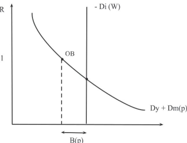
K E h i1=2 .The intuition for the existence of the Outside Bubble can be seen inFig. 4. Thisfigure represents the steady state bond
market. The vertical line is the demand of assets. The downward slopping line is the supply of assets. Given assumption A1, the equilibrium interest rate without bubbles is below one. Therefore, when the interest rate is one the supply of assets is lower than the demand of assets and a bubble may appear. In other words, the size of the bubble is the horizontal distance
between the demand of funds (savings of savers) dIand the supply of funds (borrowings of entrepreneurs)dE;yþdE;m
whenR¼1.
Finally, the equilibrium capital and consumption allocations are Km¼1
ψ
K; Ko¼ψ
ψ
1K; Co¼ψ
1ψ α
Kþψ
E: 3.2. Inside bubbleIn this subsection I compute the steady state equilibrium when there is an Inside Bubble. When there is an Inside Bubble, I assume that savers, instead of coordinating among themselves, decide to purchase capital. Since savers do not have any production technology, they just store the capital and sell it when they are old.
The return on investing on capital is the price appreciation. Therefore, the two conditions under which an Inside Bubble can appear are the same as for an Outside Bubble.
dE;yðR¼1ÞþdE;mðR¼1ÞþdIðR¼1ÞþB¼0 andB40:
I proceed in the same manner as in Subsection 3.1. I claim that the bubble exists and then I check that it is indeed the case. Note that the bond market clearing condition is the same as with the Outside Bubble,
dE;yðR¼1ÞþdE;mðR¼1ÞþdIðR¼1ÞþB¼0:
However, the capital market clearing condition is different. When there is an Inside Bubble, savers use a fraction of their savings (the bubble) to purchase capital. That is, savers demand B
punits of capital. Thus, the market clearing condition becomes
Km1;
θ
þKo1;θ
þB p¼K:By plugging the optimal choices of entrepreneurs and savers into the market clearing conditions, wefind that14
p¼
ϕ θ
;KE;WE ! ; B¼β
1þβ
Wθ
p K mð 1;θ
ÞþKoð1;θ
Þ ; Km¼ E ð1θ
Þp; K o¼α
þð1θ
Þp ð1θ
Þp K m :It is easy to check that the size of the bubble is also positive. However, I defer this discussion until the next section, where I compare the two bubbles.
Discussion of the model: Before deriving the main results of the paper, I discuss some features and assumptions of the model.
First, the source of rational bubbles in the model is thefinancial market imperfection. Entrepreneurs arefinancially constrained, which limits how much they can borrow and it constrains the supply of assets. This market incompleteness creates the shortage of assets that makes bubbles possible. Thus, to eliminate the emergence of bubbles or reduce their size, the best policy option would be to improvefinancial markets (i.e., increase
θ
). This is exemplified by the need to make assumption A1. Indeed, ifθ
were higher thanθ
, bubbles would not be possible in equilibrium.Given this shortage of assets, savers need to look for alternative ways to transfer wealth to the future. This problem was highlighted in the seminal paper ofSamuelson (1958). My Outside Bubble is analogous to his solution to this problem (money). That is, the Outside Bubble is a costless asset that savers can use to transfer wealth to the next period. Since its gross return is one (there is no population nor endowment growth), it will be purchased in equilibrium only when there is a shortage of assets that drives the interest rate below one. The second option, Inside Bubble, is that savers purchase capital (houses). Savers do not derive utility from owning capital. The only reason why savers purchase capital is to transfer wealth to the next period. Young savers buy this asset only to sell it when they will be old.
Finally, given the above reasoning, it is straightforward to see that adding a renting option would not help savers. In other words, since savers only purchase capital (houses) for the capital gains, they would not want to rent it. Thus, to incorporate renting into the model, I would need to assume that savers have to live in a house. In the Appendix, I briefly sketch how the shortage of assets could be exacerbated in this case.
4. Switching bubbles: from Outside to Inside Bubbles
In this section, I study the effects of switching from an Outside Bubble to an Inside Bubble.
Following with the motivation of the paper, it could be argued that the U.S. was in a steady state with a Dot Com Bubble in the late 1990s. However, investors realized in 2000 that they would not be able to sell the stocks of these Dot Com companies at a higher price. Thus, they decided to buy houses instead (Housing Bubble). That is, there was a shortage of assets in the economy that needed to befilled and the Dot Com Bubble was replaced by the Housing Bubble.15
To translate this narrative into the model, I proceed as follows. I assume that the economy starts in the steady state equilibrium with an Outside Bubble. In this equilibrium, young savers are happy to buy the costless asset because they think that they will be able to sell it to the next generation of young savers in the next period. In other words, savers coordinate to the Outside Bubble equilibrium.
However, all of the sudden, there is an unexpected“sentiment”shock. Young savers become pessimistic and decide not to buy the costless asset.16Instead of buying the costless asset, they coordinate to purchase capital. Given that without bubbles the interest rate is below one (assumption A1), purchasing capital is better than purchasing bonds (Inside Bubble).
14
It can be shown thatp ϕ θ;K
E;WE ð1 θÞbþ ð1 θÞ2b2þ4 1ð θÞαK E 1=2 2 1ð θÞK E whereb 2þ1βþβW E. 15
The idea that the bust of the Dot-Com Bubble was the origin of the Housing Bubble was present in both the economic media (e.g,Krugman, 2005)
and policy circles (e.g,Caballero, 2006). 16
Thus, the Outside Bubble gets replaced by the Inside Bubble.17It would be very interesting to endogenize this switch,
instead of assuming“sentiment”shocks. However, this is beyond the scope of this paper and I leave it for future research.
I make two additional assumptions to characterize the effects of the switch. Thefirst assumption is that prices are fully
flexible. It implies that the price of capital immediately adjusts to the new steady state. The second plausible assumption is
that entrepreneurs are leveraged. It means that the value of production is lower than the debt (i.e.,
α
KmoDE;y).18We are now ready to analyze how the economy is affected by switching from an Outside to an Inside Bubble. 4.1. Investment
In this subsection I study the effect of the switch on the productive investment. PanelaofFig. 5shows that prices
immediately adjust to the new steady state. Prices with an Inside Bubble are higher than those with an Outside Bubble because now there is an extra demand for capital (savers purchase capital as a store of value).
Panelbrepresents the evolution of investment of young entrepreneurs,
Km¼ E
ð1
θ
Þp: ð6ÞNote that it falls at impact to the new steady state level. The reason is that young entrepreneurs do not have capital. Thus, all the effects are through the user cost of capital: investment falls because prices are higher.
Panelcrepresents the evolution of the investment of middle aged entrepreneurs,
Ko¼ð
α
þpÞK mDy
ð1
θ
Þp : ð7ÞIt increases at impact and then it converges to the new lower steady state. At impact, the amount of capital that they
purchased when they were young,Km, and the debt,Dy, arefixed. Thus, higher prices raise investment because the increase in
net worth (the numerator) is higher than the increase in the user cost of capital (denominator). This result is due to the
assumption that entrepreneurs are leveraged (i.e.,
α
KmoDE;y). Nonetheless, investment is lower in the new steady state. TheFig. 5.Switching bubbles: From Outside to Inside Bubbles. Notes: In this exercise I assume that the price of capital directly adjusts to new steady-state.
17
Note that there exists an indeterminacy of different types of bubbles. Since both bubbles have the same return, the saver is indifferent between the
two and the two could coexist. However, I assume, consistent with the data, thatfirst there was the Outside Bubble and then the Inside Bubble. For a
further discussion on indeterminacy of bubbles, see, for example, the equilibrium with“bubble substitution”inTirole (1985)or Example 4.1 inSantos and
Woodford (1997).
18
reason is that there are two effects. On the one hand, a higher price of capital raises the net worth of entrepreneurs. On the other hand, a higher price reduces the investment that the entrepreneur made when she was young. The second effect dominates.
Therefore, the investment of middle aged entrepreneurs is lower with an Inside Bubble.19Note that if I did not assume that the
net worth of entrepreneurs is negative, the only difference would be that, at impact, investment would also fall.
To summarize, after switching from the Outside to the Inside Bubble, the capital used by entrepreneurs (both middle
aged and old) declines. In the Appendix I show that this result does not depend on the capital supply elasticity.Section 4.3
provides suggestive evidence consistent with this prediction. 4.2. Debt and size of the bubble
This section describes the effect on the debt of entrepreneurs and the size of the bubble.
Debt: PaneldofFig. 5represents the debt of youngDyand middle aged entrepreneursDm. Borrowing of entrepreneurs is limited by the collateral constraint, therefore, it is proportional to the value of their future capital. Note that the borrowing
of young entrepreneurs is the same with the two types of bubbles. From Eq.(6), it is clear that the future income of young
entrepreneurs,pKm, is constant.
The amount that middle aged entrepreneurs borrow increases at impact. However, in the steady state, the borrowing with
the Inside Bubble is lower than that with the Outside Bubble. From Eq.(7), we can see that the pledgeable capital of middle aged
entrepreneurs has two components. The value of capital purchased when youngpKmand the leverageð
α
Km DyÞ. At impact,KmandDyare constant. Thus, an increase in the price raises the value of capital purchased when young, which increases borrowing.
Note that, in contrast to the real investmentKo, this result does not depend on the sign of the second component (leverage). In
the new steady state, the debt of middle aged entrepreneurs is lower. The intuition is that the value of capital purchased when
young is constant but the leverage decreases (
α
Kmis lower with the Inside Bubble, whileDyis the same)Therefore, the borrowing of entrepreneurs falls with the Inside Bubble. This is consistent with Fig. 3. Next section
provides additional evidence consistent with this prediction.
Size of the bubble: PaneleofFig. 5represents the change in the size of the bubble. The size of the bubble is the difference between the demand and the supply of bonds. The demand of bonds (savings) is a fraction of the endowment of savers, which is constant. The supply of bonds is the total debt of entrepreneurs. Given that the demand of bonds does not change when the economy switches between bubbles, the change in the size of the bubble is the mirror image of the change in the debt of middle aged entrepreneurs. Therefore, the size of the bubble drops at impact (it looks like a bust instead of a switch between bubbles). However, in the new steady state, the bubble is larger than in the old steady state. The next proposition shows this last result.
Proposition 1. The Inside Bubble is larger than the Outside Bubble.
Proof. To prove this result note that the size of bubble can be written as Bj¼1þββW
θ
Eξ
pj for j¼fIn;Outg, whereξ
pj ¼pj Km;jð1;
θ
ÞþKo;jð1;θ
Þh i
¼2ð1θÞpjþα
ð1θÞ2pj andInandOutstand for Inside and Outside Bubble, respectively. It is immediate
to show that
ξ
0ðpjÞo0. Therefore, sincepIn4pOut, we have thatBIn4BOut.□
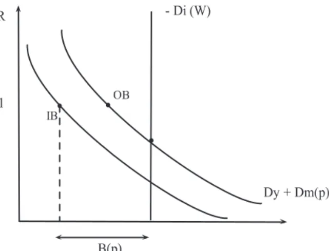
The intuition for this result can be seen inFig. 6. It represents the steady state bond market for the two bubbles. The
vertical line is the demand of bonds, which is the fraction of the endowment that savers save. The downward sloping lines, the supply of bonds, are the borrowing choices of entrepreneurs. As we have seen above, the debt of middle aged
Fig. 6.Size of the bubble: Outside and Inside Bubbles.
19
Capital of old-aged entrepreneurs can be written askoð Þp αþ ð1 θÞp
ð1 θÞp k m
p
ð Þ. Taking derivative ofkoðpÞwith respect topand noting that∂p∂kmð Þpo0, it
entrepreneurs depends negatively on the price of capital. When there is an Inside Bubble, savers purchase capital, which increases the price of capital and reduces the borrowings of middle aged entrepreneurs. Therefore, the supply of bonds falls (shifts to the left). Since when there is a bubble, the interest rate is equal to one, the difference between the demand and the supply of assets (the bubble) is higher with an Inside Bubble.
Note from the proof that only when
α
¼0, the two bubbles have the same size. The reason is that, in this case, debt is independent of the price of capital. Moreover, this result does not depend on the zero supply elasticity of capital. If I allowed for a positive supply elasticity, the rise in prices would be lower but it would still be the case that the Inside Bubble is larger than the Outside Bubble (see the Appendix for a more detailed discussion).4.3. Suggestive evidence
The main prediction of the model is that non residential investment declines when the economy switches from the Outside to the Inside Bubble. The mechanism through which this switch translates into a fall in non residential investment is the decline in the borrowing of entrepreneurs. This section provides suggestive evidence consistent with these predictions. 4.3.1. Borrowing of entrepreneurs
In the model, as the economy switches from the Outside to the Inside Bubble, the total borrowing of entrepreneurs declines. As a first piece of evidence, in the Introduction,Fig. 3 plotted the evolution of (detrended) liabilities for the manufacturing sector. Thisfigure showed that (detrended) liabilities declined during the Housing Bubble.
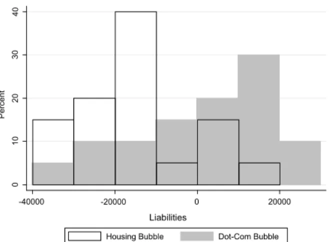
Fig. 7reports the change in the distribution of (detrended) liabilities in all sectors in the United States. As it can be seen, the distribution of liabilities shifted to the left during the Housing Bubble. One concern is that to compute the trend I also use information during the Housing Bubble, which could bias my results. To address this concern, I repeat the analysis by computing the trend before 2002 and also before 2001 (for excluding the recession too). For the manufacturing sector, the qualitative results do not change. When all sectors are considered, the median of the distribution is still lower with the housing bubble, but the mean is positive. It means that there were a few sectors with a large positive difference in (detrended) liabilities, which drive the mean. To summarize, manufacturingfirms and the median sector experienced a relative decline in borrowing during the Housing Bubble. A formal empirical analysis of the effect of the housing bubble on the credit supply is beyond the scope of this paper. However, there is an empirical paper who studies these effects for the U.S..Chakraborty et al. (2014)show that during the housing bubble, banks in more booming areas decreased commercial lending. Note that this decline in commercial lending is consistent with the prediction of model. In addition, they show thatfirms borrowing from these banks invested less. This is also consistent with the prediction of the model.
4.3.2. Non residential investment
In this section I provide more suggestive evidence that during the Housing Bubble, residential investment increased, whereas non residential investment declined.Fig. 2, in the introduction, showed that the increase in residential investment during the Housing Bubble coincided with a decline in non residential investment in the United States.
In order to complement this evidence,Fig. 8represents the share of investment in housing and house prices. The share of housing in total investment was roughly constant around 20 percent during the years of the Dot Com Bubble. At the onset of the Housing Bubble, the share sharply increased and it reached 28.7 percent in 2005. After the burst of the Housing Bubble, the share of housing collapsed. One remarkable fact of this figure is that during the Dot Com Bubble house prices also increased. However, it was not until the onset of the Housing Bubble that the rise in house prices translated into an increase in the housing share.
0 10 20 30 40 Percent -40000 -20000 0 20000 Liabilities
Housing Bubble Dot-Com Bubble
Fig. 7.Distribution of liabilities in all sectors. Notes: Thisfigure represents the distribution of differences of liabilities with respect to trend in all sectors in the two bubble episodes. It is analogous to the lines inFig. 3but with all 2-digit NAICS.
Fig. 8hints to a differential effect of house prices on the share of investment in houses depending on the type of bubble. In order to formally test this implication, I run the following regression for a sample of OECD countries,
Share residentialit¼
α
þβ
PricesitHBitþγ
PricesitDBitþδ
iþϵ
it ð8ÞwherePricesitis the house price index in countryiin timet,HBitis a Housing Bubble dummy,DBitis a Dot Com Bubble dummy and
δ
iis a set of countryfixed effects. Not all countries in the sample had a housing bubble. Thus, I construct the Housing Bubble dummy in a similar manner toJordà et al. (2015).20Since the boom in the stock market was widespread, Iassume that all countries had a stock market bubble between 1996 and 2000. The model predicts that
β
4γ
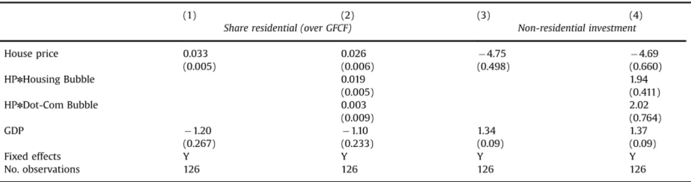
.Columns 1 and 2 ofTable 1report the coefficients of running this regression. Following with the anecdotal evidence of
Fig. 8, in column 1 I do not use the bubble dummies, but run the share of residential investment on house prices. As it can be seen, the coefficient of house prices is positive and statistically significant. In column 2, I run the main specification, Eq.(8). Consistent with the model, the coefficient of house prices is only positive and significant for the Housing Bubble episode. Therefore, this evidence is consistent with the prediction that the share of residential investment increased relatively more during the Housing Bubble.
In addition, the model also implies that there should be a differential effect of house prices on non residential invest ment. In order to test this prediction, I run the following regression,
Non residential investmentit¼
α
þβ
PricesitHBitþγ
PricesitDBitþδ
iþϵ
it ð9ÞTable 1
Housing Bubble and non-residential investment.
(1) (2) (3) (4)
Share residential (over GFCF) Non-residential investment
House price 0.033 0.026 4.75 4.69 (0.005) (0.006) (0.498) (0.660) HPnHousing Bubble 0.019 1.94 (0.005) (0.411) HPnDot-Com Bubble 0.003 2.02 (0.009) (0.764) GDP 1.20 1.10 1.34 1.37 (0.267) (0.233) (0.09) (0.09) Fixed effects Y Y Y Y No. observations 126 126 126 126
Notes: Robust standard errors in parenthesis. Share of residential (over GFCF) is the share of dwellings of grossfixed capital formation. Non-residential investment is (1-share of dwellings)*GFCF, detrended. These data come from the OECD database. I have data for house prices from 1995 to 2014. The list of countries in my sample are Australia, Canada, Spain, Great Britain, Ireland, Sweden and the United States. The housing bubble dummy is computed in a similar manner toJordà et al. (2015). The dummy is one if the detrended house price is above 1/2 of the standard deviation of the whole period and prices fall afterwards. Using this method Ifind that there were housing bubbles in the United States (2003–2007), Spain (2005–2009), Ireland (2003–2007),
Sweden (2014) and the Great Britain (2007). The Dot-Com Bubble is defined for all years and countries as happening between 1996 and 2000. The results
are robust to, for example, exogenously assume that the Housing Bubble in the United States was between 2002 and 2006 or to have an stricter bubble definition (e.g., one standard deviation instead of one half). House prices are obtained from the BIS Residential Property Price database.
100
150
200
250
House Price Index
15 20 25 30 (%Total Investment) 1995 2000 2005 2010
Dwe lings House Prices
Fig. 8.Share of investment in Housing and House Prices. Notes: Share of investment in dwellings is obtained from OECD database. House prices are
obtained from BIS Residential Property Price database.Notes: I assumeθ 0:2;β 0:6;E 10;W 20;K 10 andδ 0:6.
20
Note that this is the same type of regression as Eq.(8). The difference is that the dependent variable is non residential investment. The model predicts that
β
oγ
. Note that the results in the share of residential investment do not imply the results on non residential investment. That is, the share of non residential investment could decline with house prices during the Housing Bubble but this decline could be offset by the increase in total investment.Columns 3 and 4 of Table 1report the coefficients of running this regression. In column 3 I do not use the bubble dummies but only house prices. Note that the coefficient is negative and statistically significant. In column 4, I add the two bubble dummies. The coefficient on house prices remains negative and significant. The coefficient is smaller during the Housing Bubble, but this difference is not statistically significant. However, the correlation between house prices and non residential investment is negative for Housing Bubble episodes ( 0.84) and positive during the Dot Com Bubble (0.27), which suggests that the negative effect of house prices on non residential investment is larger during Housing Bubble episodes.
The evidence presented in this section paints a picture consistent with the model. That is, during the Housing Bubble, manufacturingfirms were able to borrow relatively less, which translated into a relative decline in both the share of non residential investment and total non residential investment. It would be interesting to formally analyze the effect of dif ferent bubbles on the borrowing and investment choices offirms. In order to do that,firm and bankfirm relationship data would be required.
5. Welfare analysis
This section performs welfare analysis. First, I show that steady state consumption is always higher with an Outside Bubble. Then, I analyze which bubble a social planner would choose and how this choice depends on the productivity of entrepreneurs.
5.1. Steady state consumption
This subsection proves that steady state consumption is higher with an Outside Bubble. Proposition 2. Steady state consumption is higher with an Outside Bubble.
Proof. To prove this result, remember that the interest rate is one with both types of bubbles. Therefore, savers are indifferent between both bubbles. The consumption of an old entrepreneur is Cj¼
α
þð1θ
ÞpjKold;j¼Γ
ðpj;θ
Þ for j¼fIn;Outg, whereΓ
pj;θ
¼ 1þ αð1θÞpj
h i2
E. It is immediate to show that
Γ
ðpj;θ
Þ is decreasing withpj. Therefore, since pIn4pOut, it follows thatCOut4CIn. □
The reason for this result is the following. First, savers are indifferent between the two bubbles because they earn the same return (R¼1). Then, there are two effects on the consumption of entrepreneurs: price and quantity. On the one hand, when there is an Inside Bubble, the extra demand for capital raises the price of capital, which increases consumption. On the other hand, with the Inside Bubble, the competition for capital reduces the amount of capital that entrepreneurs purchase, which reduces consumption. The second effect always dominates. Thus, steady state consumption is higher with an Outside Bubble.
5.2. Which bubble a social planner would choose?
In this section I consider that the economy is in a steady state without a bubble and it can switch to a steady state with either an Inside Bubble or an Outside Bubble. I show that a social planner would choose to switch to an Inside Bubble when productivity is low. I assume that a social planner cares about the consumption of all future generations. In particular, she maximizes Welfaret¼ X1 t 0
δ
t uðcEt;oÞþuðcItÞ h i ; wherecE;ot is consumption of old entrepreneurs andct I
is consumption of savers. As I have said above, since the interest rate is the same with both bubbles, the consumption of savers does not change. Thus, the social planner only needs to maximize the consumption of old entrepreneurs.
If at timetthe economy coordinates to bubblej¼fIn;Outg, thefirst generation of old entrepreneurs will see that the price of their capital ispj. The capital and price of capital for the next generations will be the steady state valuesðpj;KjÞ . Therefore, a social planner chooses an Inside Bubble if
C p In;KNB þ
δ
1δ
C p In;KIn ZC p Out;KNB þδ
1δ
C p Out;KOut :By using the consumption functions derived inSection 3, it follows that an Inside Bubble is better if KNBpIn pOutZ
δ
1δ
α
1θ
K Out KIn þ pOutKOut pInKIn : ð10ÞThe left hand side of Eq.(10)is the relative benefit of having an Inside Bubble and the right hand side is the relative loss. It cannot be proved analytically that under any configuration of the parameter space one type of bubble is better. To give an example, consider the parameter
δ
. Whenδ
¼0, the social planner only values the consumption of thefirst generation and an Inside Bubble is always better. The reason is that the price of capital is higher with the Inside Bubble. On the other extreme, whenδ
¼1, the social planner only values the consumption of the future generations and an Outside Bubble is always better. The reason is that steady state consumption is higher with an Outside Bubble (Proposition 2). The com parative statics I want to emphasize is how changes in the productivity of entrepreneurs affect the choice of the social planner.Proposition 3. As productivity decreases, an Inside Bubble becomes relatively better than an Outside Bubble.
This result can be graphically seen inFig. 9. The darker line is the left hand side of Eq.(10)and the lighter line is the right hand side of Eq.(10). Note that when productivity is very high (in thefigure,
α
¼3), the two lines are at zero. The reason is that at this productivity level the size of the bubble is zero. In thisfigure the two lines only cross once atα
¼α
. When productivity is below (above)α
, the benefit of having an Inside Bubble is larger (lower) than the loss, therefore, the Inside (Outside) Bubble is better. The intuition for this result is as follows.The relative benefit of having an Inside Bubble is the price differencepIn pOut, which is decreasing with the productivity. As productivity increases, the borrowing of entrepreneurs increases, which reduces the size of the bubble. Since the size of the bubble is small, the relative increase in the price of capital and, thus, relative benefit of the Inside Bubble, is smaller. This can also be seen in the proof ofProposition 1.
The relative loss of having an Inside Bubble is the consumption difference in the steady state, which has an inverse U shape. When productivity (
α
) is very low, the effect of the price of capital on the borrowing of middle aged entrepreneurs is small. Thus, the consumption of old entrepreneurs is very similar with both bubbles. Even though the bubble is very large pOut⪡pIn, the value of investment is very similar,pOutKOutCpInKIn
. When productivity is very large, the two bubbles are very small and the negative effects of the Inside Bubble are also small. That is,pOutCpInandKOut
CKIn. For intermediate values of productivity, the effect of higher prices on the borrowing of middle aged entrepreneurs is high. In this case, investment falls (KInoKOut) and it is not compensated by higher prices. That is,pOutKOut
4pInKIn .
Therefore, an Inside Bubble is better when productivity is low. When productivity is low, the bubble is large, which means that the gain of thefirst generation of old entrepreneurs is large. Moreover, the loss of next generations is small because the fall in capital is offset by the increase in its price. In other words, an Inside Bubble is inefficient because some capital, instead of being used to produce output, it is purchased for savers as a store of value. This inefficiency is higher, the more productive the entrepreneurs are. Therefore, the more productive an economy is, the worse it is to have an Inside Bubble.
5.2.1. Complementarity of productivity andfinancial institutions
In this section I ask in which countries a social planner is more likely to choose one type of bubble over another. In order to answer this question I interpret the tightness of the collateral constraint,
θ
, as an index of the quality offinancial institutions. The idea is that in morefinancially developed countries, the problem of limited enforcement is less severe and, thus, lenders ask borrowers a lower fraction of capital as collateral.
Proposition 4. An Inside Bubble is better in lessfinancially developed countries.
Fig. 10represents how the relative benefit and loss of having an Inside Bubble is affected by the level offinancial institutions (
θ
). The dotted line represents an economy with a lower level offinancial development. Note that the Inside Bubble would be chosen for a wider range of productivity values in the economy with a lower level of financial development.The intuition for this result follows fromPropositions 1 and 3.Proposition 1implies that countries with lessfinancially developed institutions (low
θ
) have larger bubbles. Therefore, given productivity, the size of an Inside Bubble is larger in lessfinancially developed countries. Then,Proposition 3says that Inside Bubbles are relatively better when productivity is low. This implies that Inside Bubbles are better in less financially developed countries when productivity is low. Thus, the productivity level
α
that equals the welfare of both bubbles decreases withθ
.21That is, the range of productivity levels (α
)in which an Inside Bubble is better than an Outside Bubbleð0;
α
Þis larger in lessfinancially developed countries. This can be seen inFig. 11. In this sense, an Inside Bubble is better in lessfinancially developed countries.Therefore, this simple model could rationalize why real estate bubbles tend to appear more often infinancially under developed countries. Moreover, according to the model, this type of bubble would be a good solution to their shortage of assets.22
6. Concluding remarks
Booms and busts of asset prices have been with us from, at least, the Dutch Tulip Mania in 1636 to the housing bubbles in different developed economies in the late 2000s (Kindleberger, 1978). Given that these episodes have been recurrent throughout history, it seems important to understand the effects of different asset price bubbles.
Fig. 11.Inside Bubbles are better in lessfinancially developed countries.
Fig. 10.Welfare: effect offinancial development.
21
It is easy to prove that, in the neighborhood ofα 0, the net gain of having an Inside instead of an Outside Bubble is larger in the country with less
financially developed institutions. The reason is that whereas the consumption of next generations is not affected by the size of the bubble, the price increase in thefirst generation does depend on the size of the bubble. Then, by a continuity argument, we can say that theαthat equals the relative
benefit and loss of an Inside Bubble decreases withθ. 22
In this paper I have focused on one important difference among asset price bubbles: the type of asset in which the bubble is attached. I developed a framework to understand the differential effect ofInside Bubbles(the asset is an input of pro duction, also used by entrepreneurs as collateral) andOutside Bubbles(the asset is costless and it is not used as an input). I view these two bubbles as stylized representations of the Housing and the Dot Com Bubbles, respectively.
I have shown that when the economy switches from an Outside to an Inside Bubble, the investment and debt of entrepreneurs decline, which is consistent with the data. Rational bubbles emerge in the model because there is a shortage of assets. In this situation, savers have incentives to purchase“useless”assets as a store of value (Outside Bubble). However, when savers think that they will not be able to sell this asset, they prefer to purchase capital as a store of value (Inside Bubble). By purchasing capital, savers affect the production side of the economy. In particular, this increase in the demand of capital hurts entrepreneurs, which can borrow and invest less.
Finally, I also showed that the two bubbles have different effects on welfare. In particular, a social planner prefers an Inside Bubble when the productivity of entrepreneurs is low. The reason is that the Inside Bubble distorts the economy because some resources, instead of being used by entrepreneurs, are being held by savers only as a store of value. When entrepreneurs are very low productive, the capital gain of thefirst generation of old entrepreneurs offsets the distortion.
To conclude, in a world with a shortage of assets, new bubbles are likely to emerge in the future. This paper has provided a framework to analyze the effects of two different bubbles. Given that these bubbles have different effects on welfare, it may be interesting to extend the model and study how governments (or central banks) could help investors to select the “right”bubble. Another potential avenue for future research would be to empirically analyze the effect of asset price bubbles on the credit supply and the allocation of inputs within industries.
Acknowledgments
I thank Alp Simsek for helpful discussions. I also thank Alberto Martin, Mart í Mestieri, Manuel Santos, Jean Tirole, the editor and three anonymous referees for useful suggestions and comments. All remaining errors are my own. I acknowledge
financial support from Banco de España and from the Ministerio de Economía y Competitividad (Spain), grant MDM 2014 0431.
Appendix A. Elastic capital supply
In the baseline model I have considered the case in which the supply of capital was inelastic. As I discussed in the main text, the main results of the paper are independent of the capital supply elasticity. However, it seems interesting to analyze how the magnitude of the effects depend on the capital supply elasticity. In this appendix I consider that the supply of capitalKt
S
is given by KSt¼K pεt;
where
ε
Z0 is the price elasticity of supply. Note that the case studied in the baseline model corresponds toε
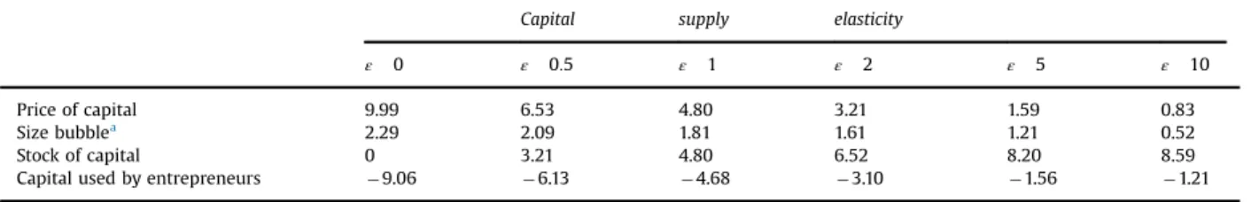
¼0.Table 1 reports the comparative statics on changing the capital supply elasticity. To be precise, each number is the percentual change of being in the steady state with an Inside Bubble with respect to an Outside Bubble.
Price of capital: Thefirst row ofTable A1shows the relative increase in the price of capital. The intuition for this result is as follows. Remember that I define an Inside Bubble as savers coordinating in purchasing capital instead of a costless asset (Outside Bubble). Assume that the size of the two bubbles were the same, it follows that the price of capital would be higher with an Inside Bubble because the demand of capital has increased. Moreover, the more elastic is the supply of capital, the lower is the increase in the price. This positive but diminishing increase of the relative price of capital is shown inTable A1. As I discussed in the main text, the size of the bubble and the price of capital are jointly determined. In particular, the Inside Bubble is larger, which exacerbates the effect on the relative price of capital.
Table A1
Comparative statics on the capital supply elasticity.
Capital supply elasticity
ε 0 ε 0:5 ε 1 ε 2 ε 5 ε 10
Price of capital 9.99 6.53 4.80 3.21 1.59 0.83
Size bubblea
2.29 2.09 1.81 1.61 1.21 0.52
Stock of capital 0 3.21 4.80 6.52 8.20 8.59
Capital used by entrepreneurs 9.06 6.13 4.68 3.10 1.56 1.21
Notes: All numbers represent percentual changes of the variable in the steady-state with the Inside Bubble with respect to the steady-state with the
Outside Bubble. I assumeθ 0:2;β 0:6;E 10;W 20 andK 10.
a
Size of the bubble: In the second row ofTable A1I show how the relative increase in the size of the bubble depends on the capital supply elasticity. AsProposition 1states, an Inside Bubble is always larger than an Outside Bubble. From the proof of
Proposition 1, it follows that the Inside Bubble is larger as long as the price of capital is higher with an Inside Bubble. When the price of capital increases, the supply of assets in the economy falls, which increases the shortage of assets that the bubble needs tofill. Note that the increase in the relative size of the bubble falls with the elasticity of capital supply. The reason is that the increase in price, as shown in thefirst row, falls with the capital supply elasticity.
Stock of capital: In the third row I report how the relative steady state stock of capital changes with the capital supply elasticity. As thefirst row showed, the price of capital is larger with the Inside Bubble. Therefore, if the supply of capital is elastic, this higher price translates into an increase in the relative stock of capital in the steady state. In addition, the more elastic is the supply of capital, the larger is the increase in the stock of capital.
Capital used by entrepreneurs: In the last row ofTable A1I compute the change in the total capital used by entrepreneurs in the steady state. We have seen that the total stock of capital is higher with an Inside Bubble because prices are higher. However, the capital used by entrepreneurs is always lower in the steady state with an Inside Bubble. The change in capital used by entrepreneurs is BIn
pInþ K
S;In KS;Out
, whereKS¼K pε. There are two effects: (i) negative competition effect: savers demand capital in the Inside Bubble, which reduces the amount available to entrepreneurs and (ii) positive supply effect: prices are higher with the Inside bubble, which increases the total supply of capital. As Table A1shows, thefirst effect always dominates. To see this, notice that when the supply is inelastic, the second effect is not there and the relative loss is the largest. When the supply is elastic, the second effect is present, which mitigates the loss but it does not eliminate it. In the limit, when the supply is very elastic, the capital used by entrepreneurs will still be slightly lower with the Inside Bubble. The reason is that, in this case, the price of capital is the same with the two bubbles, which implies that there will be the same stock of capital in the two steady states. However, the capital loss of entrepreneurs tends to zero as the capital supply elasticity increases. In other words, the Inside Bubble becomes an Outside Bubble when the supply of capital is infinite.
Appendix B. A bubbleless model with renting
In this appendix I briefly describe how renting could exacerbate the shortage of assets in the economy.
To incorporate renting into the model, I need to assume that savers enjoy utility from living in a house. Otherwise, savers would not want to rent a house. Moreover, I assume that savers cannot purchase a house, but only rent it. This extreme assumption allows me to study how the introduction of renting affects the bubbleless equilibrium described inSection 2. In the baseline model I assumed that agents do not derive utility from capital (housing) because I wanted to emphasize that they purchase capital (houses) only as a store of value.
The life time utility of a saver born a timetis Ut¼lncI tþ
β
lncItþ1þlnh I tþ1 h i :The timing of events of a saver born at timetis as follows.
1. At timet, the saver is born, she receives an endowmentWand she chooses how much to save dIt.
2. At timetþ1, the saver is old, she derives utility from living in a house and consuming thefinal good; and she dies. It means that the budget constraints of young and old savers can be written as
WþdItZcIt; 0ZcI tþ1þRtd I tþp r tþ1htþ1; wherepr
tþ1is the rental price of housing.
Finally, for making renting as innocuous as possible, I assume that there is afixed stock of capital (housing) available for rentingH, which is independent of the capital used by entrepreneursK. Thus, the problem of entrepreneurs is the same as in the baseline model.
B.1. Equilibrium
Definition. A competitive equilibrium is a sequence of prices of capitalpt, rental priceprtþ1, interest rateRt, choices of capitalkt, debtdit, consumptioncit, housing servicesh
i
tþ1for i AfI;Egfor allt40, given initial endowments of savers and
entrepreneurs and exogenous supply of capital, such that entrepreneurs maximize their utility given their income, savers maximize their utility given their income and all markets clear.
It is straightforward to derive the optimal choices of savers, cI t¼ 1 1þ2
β
W; d I t¼ 2β
1þ2β
W;cI tþ1¼
β
Rt 1þ2β
W; htþ1¼ 1 pr tþ1β
Rt 1þ2β
W:Note that optimal savings,dIt, are the same as before, except for the fact that we have 2
β
instead ofβ
. Thus, the introduction of renting is akin to decreasing the discount rate.Following the same steps as in the baseline model, the market clearing conditions for capital, renting houses and bond market, in the steady state, are
KmðR
;
θ
ÞþKoðR;
θ
Þ ¼K; H¼H;dE;yþdE;mþdI¼0:
Solving these equations, it follows that the unique equilibrium interest rate isR~NB¼rð
θ
;β
;W;E;KÞ, which is implicitly defined by23 ~ RNBθ
1þ2β
2β
W K¼Φ
R~ NB ;θ
;KE ! : B.1.1. Shortage of assetsFinally, we are interested in whether the introduction of the renting market has made bubbles less likely in equilibrium. The next proposition shows that the opposite occurs.
Proposition 5. In this model with renting, bubbles are more likely to emerge.
Proof. Note that bubbles are possible when there is a shortage of assets when R¼1. In other words, dE;yðR¼1ÞþdE;mðR¼1Þo dIðR¼1Þ. The supply of assets (left hand side) is the same as in the baseline model. However, the demand of assets (right hand side) has increased. Before, the demand was1þββW, which is smaller than12þβ2βW:Thus, for any
θ
, this condition is more likely to hold in this model than in the baseline model.□To sum up, in this appendix I have shown how the introduction of a renting sector does not solve the shortage of assets.24
The source of bubbles in the model is thefinancial friction that constrains the supply of assets. Therefore, to prevent the emergence of bubbles, the best solution is to increase the supply of assets. In the model, this could be achieved by intro ducing policies that increase
θ
. The housing model in this section was developed to highlight that renting would not solve the shortage of assets. By doing that, it abstracted from some other features. For example, in practice, both purchasing and renting coexist in equilibrium. However, this would require, for example, adding heterogeneity in thefinancial capacity of savers and introduce tax differences between renting and owning. A comprehensive model with house ownership, renting and investment offirms is outside the scope of the paper.25References
Aoki, K., Nikolov, K., 2015. Bubbles, banks andfinancial stability. J. Monet. Econ. 74 (C), 33–51. Arce, O., López-Salido, D., 2011. Housing bubbles. Am. Econ. J.: Macroecon. 3 (1), 212–241.
Azariadis, C., Smith, B., 1993. Adverse selection in the overlapping generations model: the case of pure exchange. J. Econ. Theory 60, 277–305. Bao, Z., 2015. Rational housing bubble. Econ. Theory 60 (1), 141–201.
Basco, S., 2014. Globalization andfinancial development: a model of the dot-com and the housing bubbles. J. Int. Econ. 92 (1), 78–94.
23
The capital market clearing condition can be written as R
R θEp h i 1þ R R θ αþ ð1 θÞp p h i
K, which defines a relationship between price of capital and interest rate,p Φ R;θ;K
E
. It is easy to check thatΦð:Þis decreasing withR. Similarly, the bond market clearing condition can be written asp R θ1þ2β2β
W K, which is increasing withR. Therefore, there is a unique equilibrium interest rateR~NB.
24I have assumed, consistent with the literature on housing (see, for example,Basco, 2014; and the references therein), that young agents do not derive utility from housing (e.g., they live with their parents). If I assumed that savers derive utility from living in a house in both periods, it is straightforward to see that the savings decision of savers,dI, would be exactly the same as in the baseline model. In that case,