UR Scholarship Repository
Honors Theses Student Research
2019
Rationality, revisions, and real-time data
Jason Hall
Follow this and additional works at:https://scholarship.richmond.edu/honors-theses
Part of theEconomics Commons
This Thesis is brought to you for free and open access by the Student Research at UR Scholarship Repository. It has been accepted for inclusion in Honors Theses by an authorized administrator of UR Scholarship Repository. For more information, please contact
Recommended Citation
Hall, Jason, "Rationality, revisions, and real-time data" (2019).Honors Theses. 1394.
Rationality, Revisions, and Real-Time Data by Jason Hall Honors Thesis Submitted to: Economics Department University of Richmond Richmond, VA May 1st, 2019
JASON HALL
Abstract. Revisions to macroeconomic variables are a significant part of the process by which researchers, the general public, and the government get information about the state of the United States’ economy. They are also substantial: this can have large implications for forecasting, macroeconomic research, business decisions, and monetary and fiscal policy. In this paper, I examine the cyclicality of various aggregate variables in U.S. data, and determine that of the major NIPA variables analyzed, only consumption and real imports revisions display a large degree of cyclicality. I also examine the rationality of the same set of variables under different definitions of the final value, and determine that most, though not all, of the examined variables are rational. Finally, I engage in tests of practical rationality by examining whether or not one can generate a better forecast for final release values of a variable than the initial release by incorporating information about the observed prior mean revision, and determine that incorporating this information into a model does not result in an improved forecast of final release values.
Contents
1. Introduction 1
2. Data 7
3. Results 8
3.1. Rationality and Cyclicality 8
3.2. A Fork in the Path 10
3.3. A Simple Forecasting Exercise 12
4. Conclusions 16
5. Figures 18
6. Appendix 20
1. Introduction
Virtually all major macroeconomic variables are revised. In the United States, for ex-ample, Gross Domestic Product statistics are revised by the Bureau of Economic Analysis (BEA) one month after initial release and then one month after the first revision (this revision results in so-called “first-final” estimates). Following this, the time series is up-dated yearly for roughly three years. Additionally, the BEA revises the estimates for the entire data-series approximately every five years. The difference between initial announce-ments and revised numbers can be significant. As a result of this, empirical research done with varying vintages of the same data may in fact see substantial variation in results (Croushore 2011). There has been a wide variety of work trying to document statistical properties of these revisions. The goal of this paper is to examine whether or not the direction and magnitude of revisions across key macroeconomic variables is related to the state of the business cycle, and also the extent to which those same variables are rational under different revision schemes.
This paper draws on the large literature that has developed around real-time data over the past two decades. Croushore (2011), divides this literature into two major parts: re-search emphasizing the effect of data revisions on empirical results as well as rere-search into incorporating the dynamics of revisions into the structural models endemic in macroeco-nomic research. My research is focused on the properties of revisions conditional on state in the business cycle, and this paper contributes to the former category.
A subset of the real-time data literature has focused on the rationality of various ag-gregate metrics.1
This question of whether or not initial estimates are rational is closely related to the question of whether revisions are “news” or “noise”. If later data revisions
1A release at time t
0 is rational if and only if there exists no better forecasted release value for that variable at timet0+h incorporating only data available at time t0. This set of information available at the initial release can be denoted Ωt0.
are not directly predictable using data available at the time of release, then one would expect that initial releases are rational forecasts.2
Then, since revisions necessarily re-flect information that was not available at the time of the initial release, they represent new information about the state of the economy at that point in time (hence the “news” hypothesis). On the other hand, one might think that revisions reduce noise. In this case, there is some initial measurement error in the release, new releases might reduce the discrepancy between the stated value and the true underlying value (hence the “noise” hypothesis). Another possibility, as explored by Jacobs and van Norden (2006), is that revisions are some combination of the two. Rationality tests first appear in the litera-ture in Runkle and Mankiw (1984). Keane and Runkle (1990) further develop rationality tests by dividing the hypothesis for rationality in two and then testing two different “sub-hypotheses”: one for bias and one for efficiency. There is no overall consensus on the full list of variables whose initial releases are rational; results of rationality tests can vary based on data vintage (Raponi and Frale 2014).
Most relevant to my topic is the subset of the real time literature that examines the properties of revisions around turning points in the Business Cycle. Dynan and Elmen-dorf (2001) examine GDP around recession turning points using the Real Time Dataset available from the Reserve Bank of Philadelphia. They find that GDP estimates are not fully rational, but that the gains from including additional available contemporaneous in-formation are minimal. Swanson and Van Dijk (2006) examine Bureau of Labor Statistics (BLS) statistics for industrial production and the producer price index. Notably, they are the first in the literature to examine the properties of all revisions to a variable, not just final revisions. This enables them to ascertain the extent to which initial releases are rational, but also to estimate the length of time it takes a typical variable to become
rational. They find that seasonally adjusted metrics become rational 3-8 months after their unadjusted counterparts. Additionally, they note revisions are more volatile during times of economic duress. Fixler and Grimm (2006) find that GDP estimates are not fully rational and further that revisions can be predicted by contemporaneously available in-formation. They also, however, find that this phenomenon does not appear to be present in either GDI or national income. Additionally, they note that the performance of GDP revisions becomes worse around troughs in the business cycle, but not around peaks. Abo-Zaid (2014) finds that revisions to BLS’ Net Job Creation statistics tend to vary with the state of the business cycle. He notes that initial estimates tend to underestimate final job creation numbers during expansionary periods, while they overestimate net job creation numbers during recessionary periods. This implies that net job creation numbers appear to be less volatile when viewing initial releases than they actually are.
Other elements of the literature have focused on examining basic statistical properties of revisions to aggregate variables. Runkle (1998) emphasizes the significance of using real-time data to examine policy-makers decisions by noting that revisions are large in size and initial estimates are not consistently unbiased estimates of final values.3
Aruoba (2008) notes that, optimally, final revisions4
(here being denoted as rft) would have three properties:
3Runkle emphasizes the significance of this by examining differences in the optimal interest rate in a Taylor rule computed when using initial estimates of the relevant variables versus final releases. This consideration of how revisions might be incorporated by a monetary authority is also examined by Cassou et al. (2018) who find that policymakers at the Federal Reserve target revised inflation during periods of low unemployment, but weigh heavily real-time inflation data during periods of high unemployment, resulting in a set of policy choices that appear to weigh inflation more heavily than high unemployment, despite there not necessarily being such an asymmetric preference on the part of policy-makers.
4The challenge here is that virtually all of the major macroeconomic variables are revised essentially in perpetuity. Recognizing that it is not likely that current revisions to data from 1947 actually contain any substantive new information, this suggests that we should only want to compare revisions that are relatively close in time: Aruoba chooses to make his final revisions for most NIPA variables the difference between the final yearly benchmark for that variable and its initial value.
(1) E(rtf) = 0 (2) var(rtf) is small (3) E(rtf|Ωt) = 0
He finds that none of these three properties are satisfied: revisions are not mean zero (i.e. initial estimates of the variables of interest are biased), the revisions are substantial relative to initial estimates, and further that these revisions are predictable using an information set limited to only those data available at time of initial announcement. This suggests that the initial releases of information by statistical agencies in the U.S. are not fully rational forecasts of final values of the variables.5 This paper runs somewhat contrary to earlier work by Faust et al. (2005) who find that revisions to U.S. GDP are not predictable. They also find that, in contrast to U.S. statistics, revisions to some foreign GDP measures are predictable: roughly half the variance in long-run revisions to GDP data for Italy, Japan, and the UK can be explained by incorporating data in the information set at time of initial announcement. For the countries, as well as Germany and Canada, more than a quarter of the variance in short-term revisions is explained by data in the information set at time of announcement. Preliminary announcements are also found to be significantly biased. Siliverstovs (2012) examines revisions to Swiss GDP statistics and finds that revisions to GDP growth rates are predictable using data from the Business Tendency Survey.
Sinclair and Stekler (2013) examine real GDP, nominal GDP, and the components of both to determine ex post whether or not initial releases are biased. They determine that there is partial evidence of biasedness in all of the variables considered. Raponi and Frale (2014) examine the properties of all revisions to the initial release of Italian GDP using
data provided by the Italian National Statistical Office. They conclude that revisions are not fully rational.
Revisions may also be used to better forecast future values of a variable. There are two possible approaches to take: the factor model or the state-space model. The idea be-hind the former is relatively simple: if a researcher has a substantial number of different variables that all are related in some way to the underlying state of the economy, then one could, in principle, attempt to extract the underlying state, contingent on measure-ment errors being uncorrelated between the different variables.6 Faust and Wright (2009) examine the performance of large factor models relative to the Greenbook7 forecasts and determine that the Greenbook performs better. Additionally, they determine that the gains from the large factor models are less than the gains to forecast accuracy from just averaging a large number of forecasts created by small models. Another possible approach is the use of State-Space models: these impose a data-generating process as well as the revision process in order to create a more structured model (and, hopefully, thereby im-prove forecasts). To the extent that revisions result in better estimates of the underlying macroeconomic conditions, incorporating revisions in the model might lead the model to more accurately predict future levels of the variable (for instance, if initial estimates un-derstate real GDP three quarters ago, incorporating the upward revisions might lead a model to predict relatively higher real GDP in the next period).8 This approach is used by Raponi and Frale (2014) to build a model to “nowcast” GDP.9
6If revisions are consistently biased in the same direction across all of the variables that one is pulling the
factor from, then the estimate of the factor will also be biased (Croushore 2011, Stock and Watson 2002).
7The Greenbook is a collection of the various projections and models generated by the various Federal
Reserve institutions to be used by policymakers. It is released to the public after five years have passed.
8Faust et al. (2003) note that it is possible to forecast real exchange rates using some vintages of data
but not others, and that it is not possible to effectively forecast real exchange rates using revised data.
One of the other methods used to forecast future macro values relies on predictions generated by Dynamic Stochastic General Equilibrium (DSGE) models. Such forecasts can be promising alternatives to traditional time-series forecasting methods or other tech-niques (e.g. a Bayesian SVAR). Del Negro and Schorfheide (2013), note that a medium scale DSGE based on the model put forth in Smets and Wouters (2007) can outperform the Greenbook in relatively long-duration predictions when augmented with additional frictions. One of the underlying concerns with using DSGE models for forecasting is that a naive DSGE model will include both heavily revised earlier data, as well as initial re-leases of unrevised data. To the extent that initial rere-leases are unreliable estimates of final revised values, parameter estimates in such a model could be unreliable. One possi-ble solution to this propossi-blem is to simply limit the dataset to those observations that have already undergone the initial revision process. The length of the revision process, how-ever, in conjunction with the significant information contained in relatively more recent observations means that this is an unattractive option. Another option is to model the data revision process at the same time as the model estimates parameters. Galvao (2017) takes this approach and notes that it improves forecast accuracy.10
Forecasting the true values of an underlying variable has important policy implications, but revisions can also have potent effects on empirical studies. Croushore and Stark (2001) stress the significance of revisions by pointing out that revisions may change em-pirical research in three different ways: (1) they may change the underlying data, (2) they may change the estimated coefficients, and/or (3) they may change the estimated error structure away from the true one. All of these point to the significance of recognizing the
10Another strand of the literature has examined potential reasons why agents seem to respond to initial
releases more than final numbers. Galvao and Clemens (2010) also argue that the observation that future evolutions of GDP growth appear to be responsive to initial estimates of prior GDP growth could be a byproduct of the data-revision process.
revision process for macroeconometricians, but there is also a deep significance to under-standing these revisions for policymakers. After all, policy decisions are made in real-time. Insofar as policymakers use real-time data in arguments for undertaking a specific course of action, recognizing that initial estimates of macroeconomic variables paint a more or less rosy picture of underlying economic conditions might temper (or enhance) arguments for policy interventions. Furthermore, since firms take economic conditions into account when making decisions, knowledge of the general statistical properties of revisions might lead companies at the margin to make different decisions than they would otherwise.
2. Data
To evaluate the revisions in major variables, I make use of real-time data available through the Federal Reserve Bank of Philadelphia’s Real Time Data Center, specifically the Real Time Dataset for Macroeconomists (RTDS). I consider final revisions here, with final to be taken to mean the difference between the observation recorded in the last available vintage before a benchmark revision less the initial release value. The variables in my dataset are reported below. I note that all of my dataseries run at least nominally from the 1965Q4 vintage to the 2018Q4.11 Additionally, the RTDS’ different real-time data matrices provide observations in levels of the variable. For my analysis, I calculate annualized quarterly growth rates, and then calculate revisions in those terms: that is to say that the relevant revision to Real GDP is the difference between the initially reported growth rate in a given quarter, and the final pre-benchmark growth rate, and not the
11For all variables with the exception of real output, however, only quarter 4 observations are available
from 1965-1969. Additionally, all of the variables here are missing the 1995Q4 observation as a result of a government shutdown that was ongoing when the initial estimates of the variables were to be released. To fill in this observation, I use data from the Survey of Current Business for that period, as that data would be available to forecasters working at that point in time.
difference between the level of the variable reported initially and the level reported in the final pre-benchmark vintage.
Revision Variables
(1) Y : Real Gross Domestic Product
(2) C : Real Personal Consumption Expenditures
(3) C-D : Real Personal Consumption Expenditures: Durable Goods (4) I-NR : Real Gross Private Domestic Investment: Non Residential (5) I-R : Real Gross Private Domestic Investment: Residential
(6) RG : Real Government Spending - Total12 (7) RG-F : Real Government Spending - Federal (8) REX : Real Exports
(9) RIM : Real Imports
3. Results
3.1. Rationality and Cyclicality. I run a sequence of different tests to determine whether or not recessions are correlated with the state of the business cycle, as well as whether or not they are rational. The first of these tests for cyclicality. The estimated model is as follows:
(1) rtf =βτt+t
I takerft to be the difference between the observation recorded in the last vintage before the benchmark revision closest to original release and the observation recorded in the first
release of the data.13 I take τ to be a binary indicating whether or not the observation corresponds with a period that the United States was in a recession14, and t to be my
error term.
Due the presence of this autocorrelation15, I test all hypotheses using Heteroskedasticity
and Autorcorrelation Consistent Standard Errors.
I initially restrict the intercept of my regression to be equal to 0.16 In light of this, I consider the following hypotheses:
H0 :β = 0 HA:β 6= 0
To test this, I run an F-test on the coefficient for my recession binary, τ.
I then test each of my revision time-series’ for rationality by estimating the model:
(2) rft =α+t
and running a F-test on α using HAC standard errors with the following hypotheses:
H0 :α= 0
HA:α6= 0
Below, I provide results for each of the revision variables listed above:
As you can see, consumption and real-imports exhibit a level of cyclicality in their revisions, and federal government spending, coupled with real exports and real imports
13This means that, for instance, an observation for GDP growth in 1965Q3 in the first release of the data
- the 1965Q4 vintage - is compared to the observation for GDP growth in the same time period in the 1975Q4 vintage, as the first set of benchmark revisions in my dataset occurs in January of 1976.
14I generate the recession binary via the NBER Business Cycle Dating Committee’s list of recessions. 15Although one can observe a degree of autocorrelation in the structure of revisions, as discussed in
Croushore (2011), this tends to be poorly described by conventional univariate time series methods.
Variable Cyclicality Rationality Y 0.5515 0.101 C 0.0009 0.4458 C-D 0.1375 0.2781 I-NR 0.8724 0.1366 I-R 0.4884 0.3452 RG 0.9493 0.1538 RG-F 0.9046 0.0359 REX 0.5388 0.001 RIM 0.01 0.0285
exhibit a degree of irrationality. The latter two exhibiting irrationality is not terribly surprising in light of the fact that the initial release for both imports and exports is significantly lacking in a large amount of potentially data. As a result, BEA is forced to extrapolate from prior trends, and deviations from trend growth will show up as revisions.
3.2. A Fork in the Path. One of the central dilemmas of real-time research involving rationality tests lies in defining what constitutes the final value of the affected observation. There are a variety of choices one could make, and each has the potential to result in different results. Here I am concerned primarily with two different methods for defining the final revision, each with their own advantages and disadvantages.
Under the first of the two methods, one would define the observation that occurs in the 3rd quarter of the 3rd year after initial release as the final value of the observation.17. The advantage of this definition - which I will call the 3-year method, in light of the fact that the final value of the variable is realized approximately 3 years after initial release - is that it coincides with the revision pattern for NIPA variables outlined by the BEA itself. The disadvantage, however, is that final revisions may “jump” a benchmark revision, which coincides with redefinitions of the underlying variable. The significance of these benchmark
17That is to say that, for an observation that occurs in 1970 Quarter 1, its final value will be realized in
revisions lies in the fact that one might think of these benchmark revisions as changing the data-generating process underlying our observed data on the variable of interest. Such changes have been observed to be quite large and and do not necessarily consistently affect observations within the same vintage.18 This makes inference across benchmarks
quite challenging, and indeed can require assumptions that the data-generating processes are in some way similar, which often seem to be tenuous in light of the magnitude of short-run revisions observed across some benchmark revisions.19
The second of the two methods avoids the problem of benchmark revisions by defining as the final value the value of the observation that occurs in the last vintage prior to a benchmark revision.20 The advantage of this second approach, which up until this point has been the one used, is that it avoids the problem of benchmark revisions, and thus the significant problem of potentially variable underlying data-generating processes. The disadvantage, however, is that the period of time between a first and final value for an observation is not consistent within any of the benchmarks.21
18To see why this is not surprising, consider a redefinition of GDP that captures software as investment
whereas it had not been prior. Such a revision would have a level change (as a result of the realized software investment in prior periods), but such a level change would not be consistent across time, as software investment (and software in general) is a relatively new phenomenon. Likewise, it might have trend effects on GDP, but those would not be consistent across time.
19There is an additional logical alternative to this that resolves the problem of benchmark revisions
by dropping all observations whose 3-year final values cross a benchmark. The problem with this method is that benchmark revisions are relatively frequent, and as a result, implementing this would cut the observations available for analysis by more than 50%. Additionally, the recent shift by the BEA to release benchmark revisions in July means that the available observations would be cut even more pronouncedly in recent years. Specifically, in light of the fact that Benchmark revisions occurred in 2003Q4,2009Q3,2013Q3,and 2018Q3, all observations from 2001,2002,2006,2007,2008,2010,2011,2012, and 2015, as well as observations from quarter 1 of 2003,2009,and 2013, and the quarter 2 observation from 2003. This, coupled with the fact that the last year for which the final value has been observed is 2015, leaves only 4 full years of observations (2000,2004,2005,and 2014) in the 21st century (although other years include some observations).
20Keeping in mind that the first benchmark revision relevant to our dataset occurred in January of 1976,
this means that all of the prior observations for growth rates, from 1965 Quarter 3 onwards, take on their final values in this data vintage.
21Recognizing that a real-time data matrix is essentially an upper triangular matrix, one could think of
Variable Benchmark 3-Year Y 0.1305 0.3044 C 0.5276 0.9502 C-D 0.3105 0.8231 I-NR 0.1674 0.699 I-R 0.3308 0.7106 RG 0.1453 0.8808 RG-F 0.0392 0.2046 REX 0.001 0.00003 RIM 0.02767 0.2475
Above, I provide results for rationality tests comparing each data-series across its en-tirety under the two different final revision schemes.
What we observe here is that the 3-year revisions are more likely to be rational than those defined in the benchmark revision. It is important to note, however, that under either revision scheme the majority of examined variables initial releases are still rational forecasts of final values: this is good news for anyone who attempts to make decisions in real-time.
3.3. A Simple Forecasting Exercise. Suppose that we were to take for granted that revisions are practically significant and consistently biased. The question then becomes whether or not knowledge of this information enables us to generate a better forecast for the final value of an observation than just the initial forecast. One might think of this as a question of practical rationality. In this vein, consider the following forecasts of the final observation of the final release value, where final here is taken to be the 3-year final
diagonal matrix whose blocks correspond with all the observations from the last benchmark up until the vintage immediately before the next benchmark. Hence each block constitutes a smaller upper triangular matrix of observations between benchmarks, and the relevant final revision constitutes the difference between the entries on the diagonal and the corresponding entry in the rightmost (i.e. final) column.
observation.
(3) yft =yit+t
(4) yft =yti+ ¯rt+µt
Above,yft denotes the final value of the observation, yti denotes the initial release value, ¯rt
denotes the mean of all observed final revisions prior to initial release, and bothtand µt
denote the error terms in their respective model.22 If this knowledge enabled a forecaster to, at time of initial release, generate a better estimate for the final, then we would expect that the errors generated from model (4) would be smaller than those generated from model (3).23
In order to properly test this, I consider two different samples. The first one consists of the entirety of the data in which both at least one prior revision would be observed, and for which I have final values.24
Thus, my data consists of observations for 1968Q2 growth rates onwards until 2015Q4. As a robustness check, I additionally run the DM-test on a subsample of the data consisting of only those observations in the time period from 1989Q4 up to and including 2015Q4, where we have observed a significant number of final revisions.
22Taking the final release value here to be a 3-year final, as is often the case in the literature that claim
to find cases of irrationality, this implies that there are no observed final release values prior to the initial observation for GDP growth in 1968 Quarter 2 (which corresponds with the 1968Q3 vintage for GDP data), and, further, that ¯rtis constant in 1 year increments, as 3-year final observations are always released in the 3rd Quarter of a year.
23Note as well that assuming (3) is better than (4) is roughly akin to assuming that the same GDP observation is a martingale through data vintages.
24Hence, for my output data, the tested series begins with the 1968Q2 observation (which was released in the 1968Q3 vintage, when I observe 1965Q3 and 1965Q4 final values), and ends with the 2015Q4 observation (which is the last observation for which we have final values.)
Across both of the samples, I generate a prediction using the augmented forecast, then compare the forecast errors under that regime to observed revisions (which constitute the forecast errors under the assumption that initial releases are an optimal forecast of final values) using a Diebold-Mariano test with the forecast horizon specified to be 13 periods ahead (as would be the case if you were trying to predict the 3-year final value of a Q1 observation) and an absolute value loss function. Below, I have a provided a table for p-values of results under the hypothesis that the martingale forecast - (3) - constitutes a worse forecast than the augmented forecast (4).25
Variable Full 90s Subsample Y 0.8034 0.9249 C 0.820 0.975 C-D 0.9852 0.9132 I-NR 0.9859 0.965 I-R 0.5597 0.9675 RG 0.9324 0.8734 RG-F 0.8083 0.6741 REX 0.7487 0.703 RIM 0.6875 0.1405
As you can see, in none of the cases does the martingale forecast underperform the augmented forecast at any conventional significance level. It is, however, important to keep in mind a few caveats here. The first is that the Diebold-Mariano test, by construction, typically makes use of a definite forecast window.26 Such a fixed forecast window is by its very nature not available here, as the final release NIPA variables for any given year are all released at the same time, despite the initial releases becoming available at different points in time. The second problem faced is a more general problem involving all attempts
25Put more directly, the alternative hypothesis under my test is that the martingale forecast is less accurate than the augmented forecast.
26That is to say that the Diebold-Mariano test typically supposes that all forecasts be for some fixed
to use conventional forecast comparison methods involving real-time data, namely that the conditions required for the validity of the tests are quite stringent, and that the same forecast tests are, in general, lower power than when applied to non-real time forecasts.27 Keeping this in mind, perhaps it is not the case that the optimal use of the observed mean revision is simply adding that to the observed initial release. In keeping with this possibility, I now engage in a less restrictive forecasting project, where instead of specifying that my alternative forecast consists of the initial value plus the observed mean revision, I generate a forecast for the revision by regressing historical values of the observed revision on the observed mean revision.28 I then augment the initial release value by the predicted revision generated by this model in order to generate a final predicted value for the observation of interest. Formally, this means that I am estimating the model given by:
(5) rft =α+βtr¯t+t
It is important to note here that βt is subscripted. This is because (5) is estimated
recursively.29 I then use (5) to predict a revision based on the observed mean revisions
available to a forecaster at that point in time, and then generate my final forecast for the observed value by adding the predicted revision to the initial release value. This means
27For more precise details on these issues and the assumptions required, see Clark and McCracken (2009). 28In order for this to be a valid forecasting exercise, I use only final revisions that have already been
observed at the time of initial release to train my model.
29By this I mean that I estimate the model (5) based on information available at the time of initial release.
As I move forward through time, I re-estimate equation (5) with the new information about observed revisions as it would have become available to a forecaster working in that time-period. As with the above case where ¯rt was constant in one year incremenets, my predicted rˆtf will also be constant in one year increments, as new information on which to train (5) becomes available only in the quarter 3 vintages of a year.
that my final forecast is given by the following:
(6) ytf =yti+rˆtf +t
Where rˆft is the revision predicted by equation (5) based on the observed mean revision available at the point in time when yti was released. I also note that the nature of this exercise necessitates restricting the dataset of predicted values to those that occur in 1990 vintages and onward in order to estimate (5) on a sufficiently large dataset. The question of interest thus becomes, is (3) a worse model than (6)? As with above, I test this using a DM-test with the forecast horizon 13 periods ahead under absolute error.
Variable p-values Y 0.9229 C 0.4817 C-D 0.7771 I-NR 0.1881 I-R 0.998 RG 0.861 RG-F 0.7057 REX 0.7615 RIM 0.1361
As demonstrated in the table above, none of the variables considered allow us to reject the null that the martingale forecast is not a worse forecast at any conventional significance level. Hence, all variables pass this less-restrictive test of practical rationality. Observed prior mean revision does not seem to add value to the initial forecast simplicatur.
4. Conclusions
Revisions to macroeconomic variables are, as discussed, of significant importance to anyone seeking to use that data. One of the key metrics that we associate with “reliable” revisions is that initial releases are rational forecasts of final values. Knowing that these
data are reliable in real time, then, should serve to vindicate those who are concerned with making decisions based on the fundamentals that these variables are designed to represent. Broadly, this paper has demonstrated three things. The first of these is that revisions to the majority of the examined macro-variables are not cyclical. With that said, it is important to keep in mind that the degree to which consumption and real imports do in fact appear to be cyclical. Any decisions made with these particular variables - Real Personal Consumption Expenditures and Real Imports - in mind should take this into account.
The second is that, under two different standard schemes for defining the final revi-sion, the majority of macro-variables examined here are rational. As policymakers make information in real-time, it is important that initial releases of variables of interest are reflective of values that are made with access to more relevant data (i.e. true or “final” values). The rationality finidngs here support the belief that this is actually the case.
Thirdly, it is important to keep in mind whether or not we could improve the initial releases of data, as more accurate initial releases enable everyone who seek to use the data - from policymakers to business executives - to better calibrate their decisions to the true underlying state of the economy. In the case of the examined variables here, observed prior mean revisions do not appear to provide additional information that one could use to generate an improved forecast of final values. The examined macro-variables are practically rational.
5. Figures
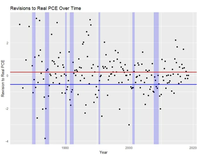
Figure 1. Revisions to Real Personal Consumption Expenditures over Time
The blue bars in Figure 1 denote recessions, the dates of which were taken from the NBER Business Cycle Dating Committee’s webpage. The red horizontal line denotes the mean revision outside of recessions, while the blue line denotes the mean during recessions. All revisions are calculated using the benchmark final scheme.
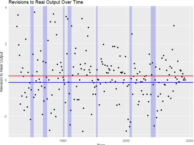
Figure 2. Revisions to Real Output over Time
The labeling scheme in this picture matches that in consumption. Note the considerably more moderate degree of cyclicality observed in output revisions than in consumption revisions. As with consumption, the revisions here are calculated using the benchmark final scheme.
6. Appendix
Below, I provide a table with descriptive statistics for all of my variables (under the benchmark final revision scheme).
Variable n Mean Min Max Y 213 0.1459 -2.84 3.728 C 200 0.0718 -3.839 3.476 C-D 200 0.283 -10.159 12.020 I-NR 200 0.594 -12.319 11.789 I-R 200 0.427 -30.678 26.885 RG 200 -0.234 -7.488 10.611 RG-F 200 -0.624 -20.067 16.598 REX 200 1.415 -18.328 24.095 RIM 200 0.902 -15.654 26.392
And here I provide a table with descriptive statistics for all of my variables under the 3-year revision scheme.
Variable n Mean Min Max Y 202 0.123 -5.087 6.703 C 189 -0.0007 -3.756 4.967 C-D 189 0.077 -11.385 12.020 I-NR 189 -0.173 -14.369 14.343 I-R 189 0.199 -34.701 26.885 RG 189 -0.0323 -7.516 10.611 RG-F 189 -0.518 -20.066 16.598 REX 189 2.092 -18.327 21.702 RIM 189 0.612 -42.951 33.087
I also ran an additioanl sensitivity test for cyclicality. Due to concerns that irrationality in
the initial release might pollute the estimate of β in the case where I fixed α to be 0, I ran an
additional specification where I allowed α to vary, and specifically evaluated the significance of
β, again using a F-test with HAC standard errors. This means that my model was the following:
With the following hypotheses of interest:
H0 :β = 0
HA:β 6= 0
I provide results for this cyclicality test below.
Variable F-stat p-value Y 1.6754 0.197 C 16.545 0.00007 C-D 4.8087 0.029 I-NR 0.8345 0.3621 I-R 0.1773 0.6741 RG 0.9674 0.3265 RG-F 0.7127 0.3996 REX 0.7563 0.3855 RIM 15.797 0.0001
Note that both of the variables that were observed to be cyclical under the rationality as-sumption remain cyclical under the new, less constrained specification. Additionally, durable consumption is observed to be cyclical under this alternative specification. Given that durable consumption is not observed to be irrational when tested separately, however, I think the ap-propriate specification is the one listed in the main body of the paper.
7. Bibliography
Abo-Zaid S (2014) “Revisions to US Labor Market Data and the Public’s Perception of the Economy.” Econ Letters 122, 119-124.
Aruoba B (2008) “Data Revisions Are Not Well Behaved.” J Money Credit Bank 40, 319-40. Clark T, McCracken M (2009) “Tests of Equal Predictive Ability With Real-Time Data.” J Bus Econ Stats 27, 441-454.
Croushore D, Stark T (2001) “A Real Time Data Set for Macroeconomists.” J Econometrics 105, 111-130.
Croushore D (2011) “Frontiers of Real-Time Data Analysis,” J Econ Lit 49, 72-100.
Cassou S, Scott P, Vasquez J (2018) “Optimal Monetary Policy Revisited: Does Considering US Real-Time Data Change Things” Appl Econ 50, 6203-6219.
Del Negro M, Schorfheide F (2013) “Chapter 2 - DSGE Model-Based Forecasting” Handbook Econ Forecasting 2, 57-140.
Dynan K, Elmendorf E (2001) “Do Provisional Estimates of Output Miss Economic Turning Points?” FRB Board Econ Finance Disc Paper 2001-2052.
Faust J, Rogers JH, Wright JH (2003) “Exchange Rate Forecasting: The Errors We’ve Really Made.” J Intl Econ 60, 35-59.
Faust J, Rogers JH, Wright JH (2005) “News and noise in G-7 GDP announcements.” J Money Credit Bank 37, 403-419.
Fixler D, Grimm B (2006) “GDP Estimates: Rationality Test and Turning Point Perfor-mance.” J Product Anal 25, 213-229.
Frale C, Marcellino M, Mazzi GL, Proietti T (2010) “EUROMIND: a monthly indicator of the Euro area economic conditions.” J R Stat Soc Ser A Stat Soc 174, 439-470.
Galvao AB, Clemens MP (2010) “First announcements and real economic activity.” Euro Econ Rev 54, 803-817.
Garratt A, Vahey S (2006) “U.K. Real-Time Macro Data Characteristics.” Econ J 116, 119-135.
Keane MP, Runkle DE (1990) “Testing the Rationality of Price Forecasts: New Evidence from Panel Data.” Am Econ Rev 80, 714-735.
Mankiw NG, Runkle DE (1984) “Are Preliminary Announcements of the Money Stock Ra-tional Forecasts?” J Monet Econ 14, 15-27.
Raponi V, Frale C (2014) “Revisions in official data and forecasting.” Stats Methods Appl 23, 451-472.
Runkle D (1998) “Revisionist History: How Data Revisions Distort Economic Policy Re-search.” FRB Minneapolis Quarterly Rev 3-12.
Siliverstovs B (2012) “Are GDP Revisions Predictable? Evidence for Switzerland.” Appl Econ Q 58, 299-326.
Sinclair TM, Stekler HO (2013) “Examining the Quality of Early GDP Component Esti-mates.” Int J Forecast 29, 736-750.
Smets F, Wouters R (2007) “Shocks and Frictions in US Business Cycles: A Bayesian DSGE Approach.” Am Econ Rev 97, 586-606.
Stock J, Watson M (2002) “Macroeconomic Forecasting Using Diffusion Indexes.” J Bus Econ Stat 20, 147-62.
Swanson NR, van Dijk D (2006) “Are Statistical Reporting Agencies Getting It Right? Data Rationality and Business Cycle Asymmetry.” J Bus Econ Stat 24, 24-42.
Jacobs J, van Norden S (2006) “Modeling Data Revisions: Measurement Error and Dynamics of True’ Values.” University of Groningen CCSO CER Working Paper.