CEP Discussion Paper No 639
May 2004
Revised January 2006
Monetary Policy and Welfare in a Small Open Economy
Bianca De Paoli
Abstract
This paper characterizes welfare in a small open economy and derives the corresponding
optimal monetary policy rule. It shows that the utility-based loss function for a small open
economy is a quadratic expression in domestic inflation, output gap and real exchange rate. In
contrast to previous works, this paper demonstrates that welfare in a small open economy,
completely integrated with the rest of the world, is affected by exchange rate variability.
Consequently, the optimal policy in a small open economy is not isomorphic to a closed
economy and does not prescribe a pure floating exchange rate regime. Domestic inflation
targeting is optimal only under a particular parameterization, where the unique relevant
distortion in the economy is price stickiness. Under a general specification for preferences
and in the presence of inefficient steady state output, exchange rate targeting arises as part of
the optimal monetary plan.
JEL Classification: F41, E52, E58, E61
Keywords: Welfare, Optimal Monetary Policy, Small Open Economy
This paper was produced as part of the Centre’s Globalisation Programme. The Centre for
Economic Performance is financed by the Economic and Social Research Council.
Acknowledgements
I would like to thank Gianluca Benigno, Nobu Kiyotaki, Fabio Ghironi, Kosuke Aoki, Andrei
Sarychev, Lars Svensson and Massimiliano Pisani for useful comments.
Bianca De Paoli is an Occasional Research Assistant at the Centre for Economic
Performance, London School of Economics. Correspondence: Bianca De Paoli, Department
of Economics, London School of Economics, Houghton Street, London WC2A 2AE, United
Kingdom. E-mail:
Published by
Centre for Economic Performance
London School of Economics and Political Science
Houghton Street
London WC2A 2AE
All rights reserved. No part of this publication may be reproduced, stored in a retrieval
system or transmitted in any form or by any means without the prior permission in writing of
the publisher nor be issued to the public or circulated in any form other than that in which it
is published.
Requests for permission to reproduce any article or part of the Working Paper should be sent
to the editor at the above address.
© Bianca De Paoli, submitted 2004
ISBN 0 7530 1765 2
1
Introduction
Should monetary policy target the exchange rate? Numerous papers have analyzed the choice of mon-etary policy objectives in closed and open economies. In the former, the debate has mainly focused on whether in‡ation should be the unique policy target. In open economies, the characterization of optimal policy extends beyond policy makers’ decision to concentrate on domestic price distortions. More speci…cally, the role of the exchange rate in the monetary policy framework needs to be consid-ered. This work addresses this particular issue in a small open economy setting. Our results suggest that including the exchange rate as part of the stabilization goals of monetary policy can be welfare improving from a small open economy point of view.
The present work lays out a small open economy model as a limiting case of a two country dynamic general equilibrium framework featuring monopolistic competition and price stickiness. Moreover, the framework assumes no trade frictions (i.e. the law of one price holds) and perfect capital markets (i.e. asset markets are complete). This benchmark speci…cation allows us to focus on the policy implications of the following factors: (a) Calvo-type staggered price setting; (b) monopolistic competition in goods’ production and the resulting ine¢ cient level of output; (c) trade imbalances; and (d) deviations from purchasing power parity that arise from the home bias speci…cation. The framework presented here encompasses, as special cases, the closed economy setting (as in Benigno and Woodford, 2003) and the small open economy case with a speci…c degree of monopolistic competition and no trade imbalances (as in Gali and Monacelli, 2005).
The small open economy representation prevents domestic policy from a¤ecting the rest of the world and, therefore, permits us to abstract from strategic interactions between countries. We focus on understanding how monetary authorities should react to ‡uctuations in internal and external conditions, when these reactions have no feedback e¤ects.
Following the method developed by Benigno and Woodford (2003) and Sutherland (2002), we derive the loss function for a small open economy from the utility of the representative household. We show that the small open economy’s loss function is a quadratic expression in domestic producer in‡ation,
the output gap and the real exchange rate. The weights given to each of these variables depend on structural parameters of the model, and therefore, are determined by the underlying economic ine¢ ciencies. In addition, the policy targets depend on the source of the disturbance a¤ecting the economy, which includes an external shock.
The analytical representation of welfare allows for a precise qualitative analysis of monetary policy in a small open economy. The results obtained show that domestic in‡ation targeting is optimal only under a particular parameterization of the model. In cases where the economy experiences productivity and foreign shocks, a domestic in‡ation target is optimal only under a particular parameterization for the coe¢ cient risk aversion and the elasticity of substitution between domestic and foreign goods. Moreover, if …scal disturbances are also present, the optimality of domestic price stabilization further requires a production subsidy. Conversely, in the general speci…cation of the model, the exchange rate becomes part of monetary policy targets. Therefore, the policy prescription in a small open economy is not isomorphic to a closed economy and does not prescribe a pure ‡oating exchange rate regime. Moreover, the quantitative results show that for a large set of parameter speci…cations, an exchange rate peg outperforms a strict domestic in‡ation target. This result is consistent with the …ndings of Sutherland (2005). The author demonstrates that for high values of the elasticity of substitution between goods a …xed exchange rate regime leads to higher welfare than targeting domestic prices.
The results obtained in this paper add to the rich debate on optimal monetary policy. Studies such as Woodford (2002) and Woodford and Benigno (2003) were pioneer in deriving a quadratic loss function (from the utility of the representative household) for a closed economy. The authors show how distortions created by monopolistic competition a¤ect the optimality of price stabilization. In an open economy setting, Corsetti and Pesenti (2000) were the …rst to emphasize that a country might bene…t from in‡uencing its terms of trade. Benigno and Benigno (2003) illustrate the potential gains from cooperation of monetary policy between countries by analyzing the incentives of individual countries to a¤ect the exchange rate. Gali and Monacelli (2004) derive the loss function, for a particular characterization of a small open economy, which was shown to be analogous to a closed economy. The present work aims at contributing to the literature by characterizing a general loss function for a small
open economy which leads to a better understanding of the international dimension of monetary policy. The remainder of the paper is structured as follows. Section 2 introduces the model and derives the small open economy dynamics. Section 3 is dedicated to the derivation of welfare and the quadratic loss function. Section 4 analyses the optimal plan and the performance of standard policy rule. Section 5 concludes.
2
The Model
The framework consists of a two-country dynamic general equilibrium model with complete asset mar-kets. Deviations from purchasing power parity arise from the existence of home bias in consumption. The dimension of this bias depends on the degree of openness and the relative size of the economy. This speci…cation allows us to characterize the small open economy by taking the limit of the home size to zero. Prior to applying the limit, we derive the optimal equilibrium conditions for the general two country model. After the limit is taken, the two countries Home and Foreign represent the small open economy and the rest of the world, respectively.
Monopolistic competition and sticky prices are introduced in the small open economy in order to address issues of monetary policy. We further assume that home price setting follows a Calvo-type contract, which introduces richer dynamic e¤ects of monetary policy than a setup where prices are set one period in advance. Moreover, we abstract from monetary frictions by considering a cashless economy, as in Woodford (2003, Chapter 2).
2.1
Preferences
We consider two countries, H (Home) and F (Foreign). The world economy is populated with a continuum of agents of unit mass, where the population in the segment [0; n) belongs to country H
in countryH is given by1: Utj =Et 1 X s=t s t U(Cj s) V(ys(h); "Y;s) ; (1)
Households obtain utility from consumption U(C)and contribute to the production of a di¤erenti-ated goody(h)attaining disutilityV(y(h); "Y;)2. Productivity shocks are denoted by"Y;s. Moreover,
C is a Dixit-Stiglitz aggregator of home and foreign goods as
C=hv1C 1 H + (1 v) 1 C 1 F i 1 ; (2)
where >0is the intratemporal elasticity of substitution andCHandCF are the two consumption sub-indices that refer to the consumption of home-produced and foreign-produced goods, respectively. The parameter determining home consumers’ preference for foreign goods, (1 v); is a function of the relative size of the foreign economy, 1 n; and of the degree of openness, ; more speci…cally, (1 v) = (1 n) :
Similar preferences are speci…ed for the rest of the world:
C=hv 1C 1 H + (1 v ) 1 C 1 F i 1 ; (3)
with v =n . That is, foreign consumers’preferences for home goods depend on the relative size of the home economy and the degree of openness. Note that the speci…cation ofv and v generates a home bias in consumption, as in Sutherland (2002).
The sub-indicesCH (CH) andCF (CF) are Home (Foreign) consumption of the di¤erentiated
prod-1In the next sections we assume the following isoelastic functional forms: U(C
t) = C 1 t 1 andV(yt; "Y;t) = "Y;ty1+t 1+ :
Where is the coe¢ cient of relative risk aversion and is equivalent to the inverse of the elasticity of labor production.
2This speci…cation would be equivalent to one in which the labour market is decentralized. These …rms employ workers
ucts produced in countriesH and F. These are de…ned as follows: CH = " 1 n 1 Z n 0 c(z) 1dz # 1 CF = " 1 1 n 1 Z 1 n c(z) 1dz # 1 (4) CH = " 1 n 1 Z n 0 c (z) 1dz # 1 CF = " 1 1 n 1 Z 1 n c (z) 1 dz # 1 ; (5)
where >1 is the elasticity of substitution across the di¤erentiated products. The consumption-based price indices that correspond to the above speci…cations of preferences are given by:
P =hvPH1 + (1 v) (PF)1 i 1 1 ; >0 (6) P =hv PH1 + (1 v ) (PF)1 i 1 1 ; >0; (7)
wherePH (PH) is the price sub-index for home-produced goods expressed in the domestic (foreign) currency and PF (PF) is the price sub-index for foreign produced goods expressed in the domestic (foreign) currency. PH= 1 n Z n 0 p(z)1 dz 1 1 ; PF = 1 1 n Z 1 n p(z)1 dz 1 1 (8) PH= 1 n Z n 0 p (z)1 dz 1 1 ; PF = 1 1 n Z 1 n p (z)1 dz 1 1 : (9)
Moreover, we assume that the law of one price holds, therefore:
p(h) =Sp (h)andp(f) =Sp (f); (10)
currency. Therefore, equations (6), (7) together with condition (10), imply that PH = SPH and
PF =SPF. However, as equations (8) and (9) illustrate, the home bias speci…cation leads to deviations from purchasing power parity, that is,P6=SP 3. For this reason, we de…ne the real exchange rate as RS=SPP :
From consumers’ preferences, we can derive the total demand for a generic good h, produced in country H, and the demand for a goodf;produced in country F:
yd(h) = p(h) PH ( PH P " vC+v (1 n) n 1 RS C # +G ) (11) yd(f) = p(f) PF 8 > > < > > : PF P h(1 v)n 1 n C+ (1 v ) 1 RS C i +G 9 > > = > > ; ; (12)
where G and G are country-speci…c government shocks. We assume that the public sector in the Home (Foreign) economy only consumes Home (Foreign) goods and has preferences for di¤erentiated goods analogous to the ones of the private sector (given by equations 4 and 5). The government budget constraints in the Home and Foreign economy are respectively given by:
t Z n 0 pt(h)yt(h)dh=nPH;t(Gt+T rt) (13) t Z 1 n pt(f)yt(f)dh= (1 n)PF;t(Gt+T rt): (14)
We consider the case in which ‡uctuations in proportional taxes t ( t) or government spending Gt (Gt) are exogenous and completely …nanced by lump-sum transfers T rt (T rt); made in the form of domestic (foreign) goods.
Finally, to portray our small open economy we use the de…nition of vandv and take the limit for
3The literature investigating the empirical evidences of Purchasing Power Parity is vast and has shown that the short
run deviations from PPP are large and volatile (as documented in Rogo¤ (1996)). Even though our model speci…cation is in accordance with these …ndings, it dismisses the evidences of failures of the law of one price.
n!0. Consequently, conditions (11) and (12) can be rewritten as: yd(h) = p(h) PH ( PH P " (1 )C+ 1 RS C # +Gt ) (15) yd(f) = p (f) PF ( PF P C +G ) : (16)
Equations (15) and (16) show how external changes in consumption a¤ect the small open economy, but the reverse is not true. Moreover, movements in the real exchange rate do not modify the rest of the world’s demand.
2.2
The asset market structure
We assume that, as in Chari et al. (2002), markets are complete domestically and internationally. In each period t; the economy faces one of the …nitely many events, st 2 (where is the set of …nitely many states). We denote the history of events up to and including periodt byxt. Looking ahead from periodt;the conditional probability of occurrence of statest+1 is (st+1jxt). The initial realization s0 is given. We represent the asset structure by having complete contingent one period
nominal bonds denominated in the home currency. We let Bj st+1 denote the home consumer’s
holdings of this bond, which pays one unit of the home currency if statest+1 occurs and0 otherwise,
and we let Q(st+1 jxt)denote the price of one unit of such a bond at date t and state stin units of domestic currency. Therefore, consumerj faces a sequence of budget constraints given by:
P(st)Cj(st) + X st2
Q(st+1jxt)Bj(st+1) Bj st + (1 t)pj(st)yj(st)dh+PH(st)T r(st): (17)
A similar expression can be derived for the foreign economy. Households at home maximize (1) subject to (17) and their optimal allocation of wealth across the di¤erent state contingent bonds implies that
Q(st+1jxt) = (st+1jxt)UC C(s t+1)
UC(C(st))
P(st)
P(st+1): (18)
Similarly for the foreign economy:
Q(st+1jxt) = (st+1jxt)UC C (s t+1)
UC(C (st))
S(st)P (st)
S(st+1)P (st+1): (19)
Therefore, the optimal risk sharing setting implies that the intertemporal marginal rate of substitu-tion (in nominal terms) is equalized across countries.
UC Ct+1 UC(Ct) Pt Pt+1 = UC(Ct+1) UC(Ct) St+1Pt StPt+1 : (20)
Equation (20) holds in all states of nature. This speci…cation for the asset market implies that the risk arising from movements in agent’s nominal wealth is shared with the rest of the world. How-ever, because of deviations from purchasing power parity, real exchange rate movements may lead to di¤erences between home and foreign real income and, consequently, di¤erences in the evolution of consumption across borders.
2.3
Price-setting Mechanism
Prices follow a partial adjustment rule a la Calvo (1983). Producers of di¤erentiated goods know the form of their individual demand functions (given by equations (15) and (16)), and maximize pro…ts taking the overall market prices and products as given. In each period a fraction 2[0;1)of randomly chosen producers is not allowed to change the nominal price of the good it produces. The remaining fraction of …rms, given by (1 ); chooses prices optimally by maximizing the expected discounted value of pro…ts4 . Therefore, the optimal choice of producers that can set their pricep~
t(j)at timeT
4All households within a country (that can modify their prices at a certain time) face the same discounted value of
is: Et ( X ( )T tUc(CT) ~ pt(j) PH;t YH;T ~ pt(j) PH;T PH;T PT (1 T)( 1) Vy(~yt;T(j); "Y;T) Uc(CT) ) = 0 (21) Monopolistic competition in production leads to a wedge between marginal utility of consumption and marginal disutility of production, represented by (1
t)( 1)
5. We allow for ‡uctuations on this
wedge by assuming a time varying proportional tax t. Hereafter, we refer to these ‡uctuations as mark up shocks t, where t= (1
t)( 1).
Given the Calvo-type setup, the price index evolves according to the following law of motion:
(PH;t)1 = PH;t1 1+ (1 ) (~pt(h))1 : (22)
The rest of the world has an analogous price setting mechanism.
2.4
A log-linear representation of the model
In this section we present a log linear version of the model. This is done in order to obtain a simple representation of the optimality conditions derived above and illustrate the dynamic properties of the model. Moreover, we later solve the log-linearized model numerically using the algorithm of King and Watson (1998) and present a quantitative analysis of the model. We approximate the model around a steady state in which the exogenous variables("y;t,Gt, t)assume the values"y 0; G= 0; 1;and producer price in‡ation is set as H;t PH;t=PH;t 1 = 1. In addition, in this steady-stateRS = 1,
C=C , Y =Y and UC(C) = Vy(Y ;0)6. Log deviations from the steady state are denoted with a
hat.
The small open economy system of equilibrium conditions derived from log linearizing equations (6), (15), (20) and (21) is:
5Note that if there are no proportional taxation and an in…nitely elastic demand = 1:This speci…cation characterizes
the perfect competition case.
6This speci…cation implies a speci…c level of initial distribution of wealth across countries. Appendix A contains the
(1 )^pH+ RSc = 0 (23) ^ Yt= p^H+ (1 ) ^C+ C^ + RSct+ ^gt (24) ^ Ct= ^Ct + 1 c RSt (25) bHt =k Cbt+ Ybt pbH+bt b"Y;t + EtbHt+1 (26)
Equation (23) describes the relationship between domestic relative prices (pH;t=PH;t=Pt)and the the real exchange rate. Equation (24) characterizes the demand for domestic goods, withg^tde…ned as
Gt G
Y . The risk sharing condition is described in equation (25). Finally, the last equation represents the small open economy Phillips Curve. We de…ne k= (1 )(1 )= (1 + )and Ht denotes the producer price in‡ation, i.e. H;t ln(PH;t=PH;t 1). Moreover, it is clear from equation (26),
that a policy of pure domestic price stabilization, that sets bHt = 0in every state, leads to the same equilibrium allocation as the case in which prices are perfectly ‡exible, i.e. when = 0;and therefore
k! 1:
The system of structural equilibrium conditions is closed by specifying the monetary policy rule. In this paper we consider the case in which monetary policy follows an optimal monetary policy. We represent the optimal plan in the form of a targeting rule. Targeting rules, as expressed in Svensson (2005), are a description of "goal directed monetary policy". Contrary to Taylor rules, an explicit expression for the evolution of the monetary policy instrument (i.e. the nominal interest rate) is not speci…ed7. Gianonni and Woodford (2003) describe these rules as ‡exible in‡ation targets. Following
this class of rules, the central bank stabilizes movements in the target variables in order to implement the most e¢ cient allocation of resources (i.e. targeting rules are derived from a microfounded welfare
maximization problem). Moreover, apart from the case in which monetary policy is represented by an optimal targeting rule, we also consider the case in which the central bank follows standard policy rules. In particular, we analyze the performance of a producer price index (PPI) in‡ation targeting regime, an exchange rate peg, and a consumer price index (CPI) in‡ation target.
Therefore, the dynamics ofYbt;RSct;Cbt;bHt andpbH;tare determined by equations (23) to (26) together with the speci…ed monetary policy, given the domestic exogenous variablesb"y;t,bgt, btand the external shockCbt 8:
Foreign dynamics are governed by the foreign Phillips curve and foreign demand:
bt =k Cbt + Ybt +bt b"Y;t + Etbt+1 (27)
^
Yt = ^C + ^gt: (28)
The speci…cation of the foreign policy rule completes the system of equilibrium conditions, which determine the evolution ofY^t;C^ andbt. We should note that the dynamics of the rest of the world is not a¤ected by Home variables. Therefore, the small open economy can treat Ct as exogenous. Moreover, the policy choice of the rest of the world modi…es the way in which foreign structural shocks a¤ectCt9 but does not in‡uence how the latter a¤ects the small open economy.
3
Welfare
The advantage of a microfounded model is that agents’ discounted sum of expected utility provides a precise measure for welfare. That is, the small open economy objective function can be obtained from equation (1). We follow the method developed by Woodford (2003) and Benigno and Woodford (2003) and obtain a quadratic expression for equation (1). This allows us to represent the policy
8In order to retrieve the value of the nominal exchange rate and interest rate we can use households’ intertemporal
choice (i.e. the Euler equation) and the de…nition of the real exchange rate.
9For example, if the foreign authority is following a strict in‡ation target the evolution of domestic consumption is
problem in a comprehensive manner. That is, policy makers minimize a quadratic loss function subject to linear constraints. Moreover, the resulting optimal monetary policy can be expressed analytically. Alternative approaches to welfare evaluation include the computational methods described in Schmitt-Grohe and Uribe (2004), Collard and Juillard (2000) and Kim et al. (2003). These techniques are based on perturbation methods and deliver a numerical evaluation of the optimal policy problem.
We should note that the linear quadratic approach presented here take into account the e¤ect of second moments in the mean of the endogenous variables. As discussed in Benigno and Woodford (2004), this ensures that the method delivers an accurate (local) welfare evaluation tool. Another important contribution that emphasizes the relevance of second order e¤ects on the mean of variables is Obstfeld and Rogo¤ (1998).
In the appendix we derive a second order approximation to equation (1). In order to eliminate the discounted linear terms in the Taylor expansion, we use a second order approximation to some of the structural equilibrium conditions and obtain a complete second order solution for the evolution of the endogenous variables of interest. It follows that the …nal expression for the small open economy loss function can be written as a quadratic function ofYbt;RSct;and bHt :
Lto=UcCEt0 X t 1 2 Y(Ybt Yb T t )2+ 1 2 RS(RSct RSc T t)2+ 1 2 (b H t )2 +t:i:p; (29)
where the policy targets YbT
t and RSc T
t are functions of the various shocks and, in general, do not coincide with the ‡exible price allocation for output and the real exchange rate. Moreover, the weights of in‡ation, output and the real exchange rate gap in welfare losses, ; Y and RS;all depend on the structural parameters of the model. The expressions for these variables are speci…ed in the appendix. Moreover, the termt:i:p stands forterms independent of policy.
What are the economic forces behind these welfare losses? The small open economy speci…cation presented in this work is characterized by two economic ine¢ ciencies: price rigidity and monopolistic competition in production. In addition, in an open economy, domestic consumption is not necessarily equal to domestic production. In particular, movements in international relative prices can create di¤erences between the marginal utility of consumption and the marginal disutility of production that
directly a¤ect welfare10. These three factors create di¤erent policy incentives. The presence of
staggered prices brings in gains from minimizing relative price ‡uctuations (justifying the presence (bHt )2 in equation (29)). Moreover, monopolistic competition in production implies a suboptimal
level of steady state output and introduces an incentive to reduce the steady state production ine¢ ciency. Finally, there may be incentives to manage ‡uctuations in the exchange rate in order to a¤ect the wedge between the marginal utility of consumption and the marginal disutility of production (hereafter this is referred as the "Uc=Vy gap"). The last two factors imply that optimal monetary policy might deviate from price stability (and are responsible for the presence of the terms Y(Ybt YbtT)2 and
RS(RSct RSc T
t)2 in equation 29).
To better understand the argument presented above, we …rst characterize a closed economy by setting = 0. In this case, equation (29) can be written as:
Lcto=UcCEt0 X t 1 2 c Y(Ybt YbtT ;c)2+ 1 2 c( bHt )2 +t:i:p; (30)
where the subscript c denotes the closed economy. The policy maker’s problem in a closed economy can be illustrated by the relative weight of in‡ation with respect to output = Y and by the di¤erence betweenYbT
t andYbtF lex (whereYbtF lex represents the ‡exible price allocation for output). c c Y = k( + ) (31) b YtT ;c= "Y;t ( + ) ( 1)( + 1) t ( + )( + + ( 1))+ ( + )gt ( + )( + + ( 1)) (32) b YtF lex;c = "Y;t t+ gt ( + ) : (33)
As the above expressions show,YbtT ;c6=YbtF lex;c, that is, a policy of strict in‡ation targeting (which
1 0This is represented by the termU
cC(Cbt Ybt= )in the Taylor expansion of the utility function (shown in the appendix).
Note that in our linear-quadratic aproach this term is expressed in terms of second moments. In particular, it can be written as a function of the variance of the real exchange rate and output gap.
mimics the ‡exible price allocation) does not close the welfare relevant output gap. Therefore, there is a trade-o¤ between stabilizing in‡ation and output. Moreover, the weight of in‡ation relative to output in the loss function depends essentially on the degree of market power and the degree of price rigidity (which determines the parameterk). When the elasticity of substitution between goods is in…nite, i.e. the market is competitive, then the relative weight on the output gap vanishes. On the other hand, when !0 (and consequentlyk ! 1), the relative weight on in‡ation fades away as there are no distortions associated with price rigidity. Furthermore, the steady state level of mark up,
;and mark up ‡uctuations, t;imply di¤erences betweenYbT
t andYbtF lex. Whenever the steady state level of production is e¢ cient, i.e. = 1;and there are no mark up ‡uctuations, we haveYbT
t =YbtF lex: On the other hand, in a small open economy, in addition to domestic prices and output ‡uctuations, real exchange rate movements also a¤ect welfare. This is because the exchange rate can generate ‡uctuations in the so called "Uc=Vy gap". As shown in equation (24) and (23), the real exchange rate in‡uences the relative price of Home produced goods and modi…es the small open economy’s demand. Secondly, in a world where purchasing power parity does not hold, real exchange rate movements generate real wealth variations, which, in turn, create ‡uctuations in households’spending and consumption (this can be seen by inspection of equation (25)). It follows that the impact of the real exchange rate on output and consumption a¤ects the wedge between marginal utility of consumption and marginal disutility of production. And ‡uctuations in this gap have an e¤ect on the small open economy’s welfare.
The value of intertemporal and intratemporal elasticities of substitution, 1= and , determine the real exchange rate e¤ect on consumption and output through the risk sharing and demand channels explained above. Therefore, the weight of the real exchange rate in the loss function, RS, depends crucially on these parameters. More speci…cally, when = 1 the real exchange rate does not a¤ect the "Uc=Vy gap" and RS = 0. Section 4.1 explores this special case in detail. In addition, when the economy is relatively close, the welfare implications of real exchange rate movements are small (as expected, when !0; RS !0):
4
Optimal Monetary Policy
After characterizing the policy objective, we now turn to the constraints of the policy problem. The …rst constraint the policy maker faces is given by the Phillips Curve:
btH =k ( ^Yt YbtT) + (1 ) 1(RSct RSc T
t) +ut + EtbHt+1; (34)
where ut is a linear combination of the shocks de…ned in the appendix. The policy problem is further constrained by the small open economy aggregate demand equation (24) and the risk sharing condition (20). Combining these two conditions, the following relationship between output and the real exchange rate arises:
(Ybt YbtT) = (RSct RSc T t)
(1 +l)
(1 )+ ut; (35)
where l= ( 1) (2 )and is a vector whose elements depend on the structural parameters (as shown in the appendix). From equation (34) we can see that the policy targetsYbtT and RSc
T tare not necessarily the ‡exible price allocations of output and the real exchange rate. That is, the targets do not coincide with the allocations that would prevail if = 0(and consequentlyk! 1). Moreover, equation (35) shows that closing the “output gap” does not eliminate the“real exchange rate gap”.
We proceed by characterizing the optimal plan under the assumption that policy makers can commit to maximizing the economy’s welfare. We lay out the Ramsey problem and derive the optimal policy response to the di¤erent shocks. The policy problem consists of choosing a path for fbHt ;Ybt;RSctg in order to minimize (29), subject to the constraints (34) and (35), and given the initial conditionsbt0 and
b
Yt0. This last condition implies that the resulting set of …rst order conditions does not internalize the
e¤ect of previous expectations of the initial policy. This method follows Woodford’s (1999) timeless perspective approach, and thereby ensures that the policy prescription does not constitute a time inconsistent problem. In e¤ect, the constraints on the initial conditions impose that the …rst order condition to the problem are time invariant11. The multipliers associated with (34) and (35) are
respectively'1 and'2. Thus, the …rst order conditions with respect to btH;Y^tandRSct are given by:
('1;t '1;t 1) =k bHt (36) '2;t '1;t= Y(Ybt YbtT) (37) '2;t (1 +l)'1;t= (1 ) (1 +l) RS(RSct RSc T t): (38)
Combining equations (36), (37), and (38), we obtain the following expression:
(1 +l) Y (Ybt YbtT) + (1 ) RS (RSct RSc T
t) + ( + (1 +l))k (b H
t ) = 0; (39)
where denotes the …rst di¤erence operator. The above expression characterizes the small open economy optimal targeting rule. It prescribes responding to movements in in‡ation, output and the real exchange rate12. Moreover, equation (39) stipulates how monetary policy should respond to the
di¤erent shocks, according to the composition of YbT
t and RSc T
t. When following this policy rule, the central bank may allow some variability in in‡ation in order to respond to costly movements in other variables. Equation (39) indicates the policy maker’s behavior that minimizes welfare losses is associated with such ‡uctuations. It implements the most e¢ cient allocation of resources, conditional on the structural characteristics of the economy.
In the appendix we show which parametric restrictions are needed for the above …rst order conditions to lead to a determinate equilibrium. The appendix also contains an analysis of whether the above …rst order conditions indeed characterize an optimal policy. That is, section D of the appendix investigates if there is any alternative random policy that could improve welfare. As shown in Benigno and Woodford (2003), this approach coincides with the investigation of whether the second order conditions of the minimization problem are satis…ed. It follows that some parameter speci…cations violate these conditions (those are shown in table 13 and 14).
1 2Even if we express equation (39) as a function of Consumer Price Index in‡ation instead of producer price in‡ation
bH
t , the targeting rule still includes the term (RSct RSc T t).
We now turn to the analysis of some special cases of the optimal plan. Moreover, we explore how certain economic characteristics in‡uence the optimal monetary policy.
4.1
Producer Price In‡ation Target
Under certain circumstances, the loss function approximation leads to clear cut results in terms of optimal policy. In this section we analyze when optimal policy consists of PPI (producer price index) in‡ation targeting, i.e., it prescribes complete domestic price stability. The conditions under which this is true involve assumptions on the parameter values of the model and on the source of the shock present in the economy.
In order to understand the ine¢ ciency of the ‡exible price allocation in the general case and the special cases where a strict in‡ation target is optimal, it is useful to characterize the social planer’s optimal allocation. In this section we step back from the linear quadratic analysis and compare our non-linear equilibrium conditions with the social planer’s optimal allocation. The planner’s objective is to maximize agents utility Ut subject to the small open economy’s demand and the risk sharing condition, given by equations (11) and (20), and is further completed by the determination of relative prices (equation (6)). Moreover, the small open economy’s social planner takes external conditions as given. Hence, the social planner’s …rst order condition can be written as
PH;te Uc(Cte) =qteVy(Yte; "Y;t); (40) whereqe t = h 1 + ( 1) (RSe t) 1 +1 (RSe t) 1i
and the superscriptedenotes the e¢ cient allocation. The full characterization of the e¢ cient allocation can be obtained by combining the above equation with the constraints of the policy problem (i.e. equations (6), (11), and (20)). Furthermore, in steady state we have
Uc(Y e ) = 1 (1 )Vy(Y e ): (41)
competition and price stickiness is given by the price setting equation (21). If we assume, however, that prices are ‡exible, the equilibrium condition (21) becomes
pF lexH;t Uc(CtF lex) = tVy YtF lex; "Y;T ; (42)
and in steady state
Uc(Y F lex
) = Vy(Y F lex
): (43)
Therefore, comparing conditions (40) and (42), it is clear that even with perfectly ‡exible prices, mark up shocks and movements in the real exchange rate generate ine¢ cient ‡uctuations in the ratio of marginal disutility of production and marginal utility of consumption. In addition, unless = 1=(1 );
the small open economy steady state output is ine¢ cient (this can be seen by inspection of equations (41) and (43)). That is, in general, a policy of domestic price stabilization that mimics the ‡exible price allocation does not implement an e¢ cient allocation.
Nevertheless, if we impose that = 1; the e¢ ciency condition (40) and the decentralized ‡exible price allocation (42) can be written as follows
(1 ) (Yte Gt) ="Y;t(Y e
t) (44)
1 t
(YtF lex Gt) ="Y;t YtF lex : (45)
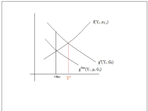
The above expressions are illustrated in Figure 1, where f(Yt; "t) = "Y;tYt , gf lex(Yt; t; Gt) =
1
t(Yt Gt) ;andg
e(Y
t; Gt) = (1 )(Yt Gt) . The ine¢ ciency of the steady state ‡exible price allocation is represented by the location of Yf lex below Ye. Moreover, apart from the steady state distortion, ‡uctuations in the wedge between ge andgF lex characterize a departure from the e¢ cient allocation given by (44) and also represent distortions present in the ‡exible price equilibrium.
even with = 1and ‡exible prices, mark up shocks generate distortions that a¤ect welfare. Hence, there is an incentive to stabilize these shocks and depart from the ‡exible price equilibrium (i.e. a strict domestic in‡ation target is not optimal).
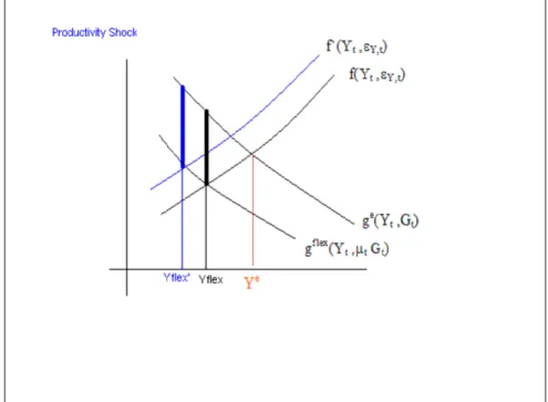
Figure 3 shows how productivity shocks a¤ect e¢ ciency. In the case of = 1, the equilibrium ‡exible price allocation and the e¢ cient allocation move proportionally to each other. This leaves the welfare relevant wedge unchanged. Therefore, there are no welfare losses under price ‡exibility and a producer price in‡ation targeting characterizes the optimal plan. The same result holds for the case of foreign shocks. External disturbances do not appear in the expressions forf(:), gF lex(:)or ge(:). Thus, these shocks also leave the wedge unchanged when = 1. The intuition behind this result is that, under this parametrization, the marginal e¤ect of the real exchange rate on consumption utility and labour disutility o¤set each other and no stabilization process is needed.
Figure 4 shows the case of exogenous ‡uctuations in government expenditure. Because …scal shocks do not a¤ectgf lex andgeproportionally, their e¤ect on e¢ ciency depends on the steady state level of output. In general, …scal disturbances create ine¢ cient movements in the wedge between gf lex and
ge;as represented in the …gure. The only circumstance in which there are no such movements is when the steady state level of output is e¢ cient (Yf lex =Y ). This result is consistent with the …ndings of Benigno and Woodford (2004) in a closed economy setting.
Therefore, the assumptions needed in order to have an in‡ation target as the optimal plan are: (1) = 1; (2) there should be no mark-up shocks ( t = 0; 8 t); and, in the case of …scal shocks, (3) the steady state level of output ought to be e¢ cient from the small open economy’s point of view (i.e. = 1=(1 )). These conditions guarantee that the ‡exible price equilibrium characterizes the e¢ cient allocation.
Under this speci…cation, the weights on the loss function are:
Y
(1 ) = ( + ) (46)
(1 )= k: (48)
And the target for output is:
b
YtT =YbtF lex= ( + ) 1f "Y;t+gtg: (49) The relative weights speci…ed in equations (46) and (48) are analogous to those in the closed economy and the policy target coincides with the ‡exible price allocation. The assumption of = 1=(1 ) guarantees that steady state output is e¢ cient from the point of view of the small open economy. In addition, the restriction of = 1, ensures that exchange rate movements do not a¤ect welfare since its the marginal e¤ect on consumption utility and labour disutility o¤set each other. Moreover, the optimal plan does not respond to external shocks. In what follows, under this speci…cation, the optimal monetary policy in a small open economy is isomorphic to a closed economy. This result is consistent with the …ndings of Gali and Monacelli (2005)13.
4.2
Quantitative results
4.2.1 The General Optimal Plan:
In this section we present some numerical analysis of the optimal monetary policy. In our benchmark speci…cation we assume a unitary elasticity of intertemporal substitution, i.e. = 1. Following Rotemberg and Woodford (1997) we assume = 0:47. Furthermore, the elasticity of substitution between home and foreign goods, , is assumed to be 314 (Obstfeld and Rogo¤ (1998) argue that it
should be between 3 and 6). The degree of openness, ;is assumed to be0:2;implying a 20% import share of the GDP. In addition, the baseline calibration considers the case of a "optimal subsidy" policy, where is set such that = 1=(1 ). Moreover, the elasticity of substitution between di¤erentiated goods is assumed to be 10 as in Benigno and Benigno (2003). To characterize an average length of
1 3The authors have characterized the loss function for a small open economy in the case in which trade imbalances or
steady state monopolistic distortions are absent (i.e. = = 1and = 1=(1 )).
price contract of 3 quarters, we assume = 0:66. Finally, we assume = 0:99. Starting from this speci…cation, we analyze how optimal monetary policy responds to the di¤erent shocks.
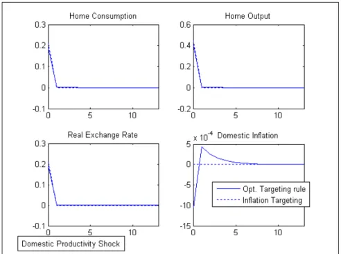
Figure 7 shows the impulse response of consumption, output, the real exchange rate and producer price in‡ation following a productivity shock. Comparing the optimal policy with an in‡ation target highlights that there are no quantitatively signi…cant di¤erences between the two. Under both regimes a higher productivity at home increases domestic output and consumption. In addition, a larger supply of domestic goods leads to a depreciation in the real exchange rate.
The zero measure speci…cation of the Home economy enables us to study how the monetary authority should respond to ‡uctuations on external conditions, when there are no feedback e¤ects. Figure 6 presents the impulse response of the various domestic variables to a foreign shock - represented by an innovation in Ct. Again, the optimal plan is quantitatively similar to an in‡ation targeting regime. Domestic consumption increases with the increase in foreign consumption and there is a real exchange rate appreciation. The impact on domestic competitiveness now leads to a fall in home production.
As illustrated in Figure 7, when the economy is subject to mark up shocks, optimal monetary policy departs from price stabilization. The optimal plan reacts to ‡uctuations in the wedge between marginal utility of consumption and marginal disutility of production. The policy response to a mark up shock implies an exchange rate depreciation and an increase in the domestic consumption of home goods. As a result, domestic output increases. As shown in …gure 8, this is not the case when the economy is closed. In this case, in‡ation stabilization is larger, requiring a contraction in the level of economic activity.
The optimal response to a …scal shock is presented in …gures 9, 10 and 1115. Figure 9 compares
the optimal monetary policy with an in‡ation targeting regime. It shows that the exchange rate depreciation is smaller in the former. Consequently, crowding out in consumption is smaller under the optimal regime. As a result, whereas output falls under a policy of price stability, domestic production increases under the optimal plan. Conversely, as portrayed in …gure 10, the optimal plan in a closed economy is closer to an in‡ation target and involves a larger fall in consumption.
1 5Given thatbg
tis de…ned as (G G)
These results change signi…cantly when the goods are complementary in utility. As displayed in …gure 11, when = 0:7, a …scal shock leads to an exchange rate appreciation and a fall in domestic consumption.
4.2.2 Ranking Standard Policy Rules
Exercises such as the ones shown above demonstrate that the source of the shock a¤ecting the economy is an important determinant of the performance of policy rules. In the optimal targeting rule, this is captured by the composition of the target variables YbT
t and RSc T
t; which stipulate how optimal policy should respond to di¤erent shocks. The quantitative analysis also illustrates the role of the economy’s characteristics (that is, variations in the structural parameters such as and ) in the policy prescription. In analytical terms this is captured by the formulation of the weights of the variables in the loss function and in the targeting rule.
In order to verify how robust the results presented in the previous section are (specially regarding the validity of producer price in‡ation targeting), some sensitivity analysis should be conducted . However, as shown in section (4) of the appendix, not every combination of parameter speci…cation is consistent with the second order condition of the minimization problem. For this reason, the computation of the optimal plan as shown above is not valid for those speci…cations. Therefore, an alternative robustness check has to be done by evaluating the performance of an in‡ation targeting regime compared with other standard policy rules for the di¤erent parameter values and types of disturbances. This exercise is also interestingper se, as it allows the evaluation of policies currently used by international monetary authorities.
We compute a ranking of policy rules (more speci…cally, domestic in‡ation targeting, CPI in‡ation targeting and exchange rate peg) for di¤erent values of ; and . We start by varying and ;while maintaining = 0:4. Alternatively, we can keep the log utility speci…cation and analyze di¤erent scenarios for and . Moreover, we consider the case of 1% standard deviation productivity, …scal and mark up shocks16.
1 6Kehoe and Perri (2000) …nd and estimate of 0.7% for the productivity shock standard deviation. Gali et al (2002) …nds
a standard deviation for price mark ups of 4.3% (implying variance of approximately 0.0016). Perotti (2005) estimates the standard deviation of a government spending shock for various countries. The estimates range from 0.8% to 3.5%.
Tables 1 and 2 show the policy rule that leads to the highest level of welfare, following a productivity shock. Domestic in‡ation targeting is the preferred policy rule for low levels of ; and . A large elasticity of substitution between domestic and foreign goods increases the sensitivity of home demand to exchange rate movements. As a result, exchange rate ‡uctuations have a higher impact on the rate of marginal utility of consumption and marginal disutility of production. For this reason, when is high, the small open economy bene…ts from adopting an exchange rate peg. The same happens when the coe¢ cient of risk aversion is large. Moreover, an exchange rate peg becomes superior to PPI or CPI in‡ation targeting when the economy is relatively open.
The gains or losses of adopting di¤erent policy regimes are represented by the following measure:
Wda;b= W a Wb Uc(C) = 2(1 )(U a 0 U0b) U(C) ;
whereU0is the expected life time utility of the representative agent. Wda;bmeasures the percentage
di¤erence in steady state consumption under regime aandb. Table 3 illustrates the welfare gains or losses of adopting an in‡ation targeting rather than an exchange rate peg when the economy is subject to productivity shocks. Although an exchange rate peg is superior to an in‡ation targeting regime when ; and are large, the quantitative welfare loss is not very signi…cant: it ranges from 0.001% to 0.004% of steady state consumption. As shown in section 5.1 when = = 1 and the economy is subject to productivity shocks, a domestic in‡ation target coincides with the optimal policy rule. In this case, the welfare losses of a …xed exchange rate regime is 0.010% of steady state consumption. Table 9 shows that these costs increase to 0.013% when the economy is relatively closed ( = 1=5):
In the case of foreign shocks, …gures for the preferred policy are identical to the case of domestic productivity shocks. Pegging the exchange rate outperform an in‡ation targeting regime when the economy is relatively open, and demand is sensitive to exchange rate movements (i.e., is large) and the intertemporal elasticity of substitution is small (high levels of ). This is illustrated in tables 5 and 6.
Turning to …scal shocks, for intermediate levels of ; and , CPI targeting is the best of the
three standard policy forms evaluated. That is, under these speci…cations, the central bank improves welfare by targeting a weighted average of domestic in‡ation and exchange rate depreciation. This is illustrated in tables 7 and 8. However, the cost of imposing an in‡ation targeting regime under this parametrization is insigni…cant: at most 0.001% loss in steady state consumption (see highlighted statistics in table 9 and 10). Moreover, as in the case of foreign and productivity shocks, when ;
and are large, …xing the exchange rate is the best alternative
In the case of mark up shocks, an in‡ation target is the preferred standard policy only under the knife-edge speci…cation where = = 1 (see table 11). With unitary elasticity of substitution and
>1;CPI targeting is the preferred policy rule. In addition, whenever >2pegging the exchange rate leads to higher welfare than PPI in‡ation targeting. The steady state consumption losses associated with strict domestic price stabilization compared with a …xed exchange rate regime are shown in table 12. When mark up ‡uctuations are the source of disturbance a¤ecting the small open economy,
WdIT ;P EGmay reach 0.043%, when = = 6.
The costs of adopting a welfare inferior policy rule presented in the above tables are small in magnitude. The shift in steady state consumption is never larger than 0.05%. We should note however that these costs are of the same order of magnitude as the costs of business cycles reported by Lucas (1987) (the author estimates a 0.1% shift in steady state consumption).
5
Conclusion
This paper formalizes a small open economy model as a limiting case of a two country general equilib-rium framework and characterizes its utility-based loss function. It also derives the optimal monetary plan, represented by a targeting rule, for a small open economy. The setup developed in this work encompasses, as special cases, the closed economy framework and the small open economy case with e¢ cient levels of steady state output. As a result, the examination of monetary policy in such envi-ronments is nested in our analysis.
The utility-based loss function for a small open economy is a quadratic expression in domestic in‡ation, the output gap and the real exchange rate. This paper demonstrates that a small open
economy, completely integrated with the rest of the world, should be concerned about exchange rate variability. Therefore, the optimal policy in a small open economy is not isomorphic to that in a closed economy and also, it does not prescribe a pure ‡oating exchange rate regime. Price stability (or domestic in‡ation targeting) is optimal only under a speci…c parameterization of the model. In the cases where the economy experiences productivity and foreign shocks exclusively, domestic in‡ation targeting is only optimal under a particular speci…cation for preferences. If …scal disturbances are also present, price stability as the optimal plan further requires a production subsidy. When these restrictions on the steady state level output and preferences are relaxed, deviations from inward looking policies arise in the optimal plan.
Nevertheless, under our benchmark calibration, the optimal monetary policy mimics closely an in‡ation targeting regime when the economy experiences domestic productivity shocks and external disturbances. In the case of …scal and mark up shocks the optimal plan departs from price stabil-ity. Moreover, the openness of the economy modi…es the optimal responses to the referred shocks signi…cantly.
The sensitivity analysis exercise demonstrates that in‡ation targeting, when comparing CPI and exchange rate targeting, is the preferred policy if the economy is relatively closed and its demand is not sensitive to exchange rate movements. Conversely, if ; and are large, the small open economy may improve welfare by adopting a …xed exchange rate regime.
The tools developed in this paper can be applied to di¤erent economic environments. It is important to notice that the model presented here assumes that there are complete asset markets. Relaxing such assumption would lead to a more realistic representation of the model. Moreover, the introduction of asset market imperfections and their welfare consequences would enrich the optimal monetary policy analysis.
Another interesting extension would involve analyzing …scal policy by allowing proportional taxation to be an endogenous variable. This would enable the investigation of the interaction between …scal and monetary authorities and the optimal policy mix. The small open economy representation allows for the assessment of interesting issues such as the implication of di¤erent government bond denominations
for …scal policy. Moreover, one could analyze optimal …scal arrangements under a …xed exchange rate regime.
References
[1] Aoki, K. (2001) "Optimal Monetary Policy Response to Relative Price Changes" Journal of Mon-etary Economics 48, pp55-80.
[2] Arseneau, D. (2004). "Optimal in‡ation in an open economy with imperfect competition" Finance and Economics Discussion Series 2004-25, Board of Governors of the Federal Reserve System (U.S.). [3] Benigno, G and Benigno,P (2003) "Price Stability in Open Economies" Review of Economic
Stud-ies, Vol.70, No. 245.
[4] Benigno, G and Benigno,P (2003) "Designing Targeting rule for International Monetary Policy Coordination" ECB working paper No. 279.
[5] Benigno, P:and Woodford, M (2003) "In‡ation Stabilization and Welfare: the Case of Large Distortions" NBER Working Papers 10838.
[6] Bowman, D. and Doyle, B., (2003) "New Keynesian, Open-Economy Models and Their Implications for Monetary Policy" FRB International Finance Discussion Paper No. 762.
[7] Calvo, G. (1983) "Staggered Prices in a Utility-Maximizing Framework" Journal of Monetary Economics, vol. 12, pages 383-398.
[8] Clarida, R., Gali, J., Getler, M.(2001) "Optimal Monetary Policy in Closed versus Open Economies: An Integrated Approach" NBER Working Paper No. W8604.
[9] Corsetti, G and Pesenti, P,.(2001) "Welfare and Macroeconomic Interdependence" Quarterly Jour-nal of Economics, vol. 116, issue 2.
[10] Corsetti, G. and Pesenti, P., (2005). "International dimensions of optimal monetary policy," Journal of Monetary Economics, Elsevier, vol. 52(2), pages 281-305.
[11] Fry, M., D. Julius, L. Mahadeva, S. Roger and G. Sterne, (2000) "Key issues in the choice of monetary policy framework", in L. Mahadeva and G. Sterne (eds.), Monetary policy frameworks in a global context, Routledge, pp 1-216.
[12] Gali, J and Monacelli, T (2005) "Monetary Policy and Exchange Rate Volatility in a Small Open Economy", Review of Economic Studies, Volume 72, Issue 3, Page 707-734.
[13] Gali, J., Gertler, M. and Lopez-Salido, J., (2002) "Markups, Gaps, and the Welfare Costs of Business Fluctuations" NBER Working Paper No. W8850.
[14] Devereux, M., and Engel, C. (2000). "Monetary Policy in the Open Economy Revisited: Price Setting and Exchange Rate Flexibility" NBER WP No. 7665.
[15] Engel, C. (2002) "The Responsiveness of Consumer Prices to Exchange Rates And the Implications for Exchange-Rate Policy: A Survey Of a Few Recent New Open-Economy" NBER Working Papers 8725, National Bureau of Economic Research, Inc.
[16] Engel, C. and Rogers,J. (1999). "Deviations from Purchasing Power Parity:Causes and Welfare Costs" Discussion Papers in Economics at the University of Washington 0038, Department of Economics at the University of Washington.
[17] Ganelli, G and Lane, P., (2002) "Dynamic General Equilibrium Analysis: The Open Economy Dimension" CEPR Discussion Papers 3540, C.E.P.R. Discussion Papers.
[18] Ghironi, F., (2003)."Macroeconomic Interdependence under Incomplete Markets" Boston College Working Papers in Economics, Boston College Department of Economics.
[19] Giannoni, M. and Woodford, M. (2003) "Optimal In‡ation Targeting Rules" NBER Working Paper No. W9939.
[20] Goodfriend, M. and. King,R.G. (2001) "The Case for Price Stability" NBER Working Papers 8423, National Bureau of Economic Research.
[21] Khan, A, King, R and Wolman, A. (2003). "Optimal Monetary Policy," Review of Economic Studies, Blackwell Publishing, vol. 70(4), pages 825-860.
[22] Kollmann, R., (2002) "Monetary Policy Rules in the Open Economy: E¤ects on Welfare and Business Cycles" CEPR Discussion Papers 3279, C.E.P.R. Discussion Papers.
[23] Lane, P. (2001), "The New Open Economy Macroeconomics: A Survey" Journal of International Economics, vol 54, pages 235-266.
[24] McCallum, B. and Nelson, E., (2004). "Timeless perspective vs. discretionary monetary policy in forward-looking models," Review, Federal Reserve Bank of St. Louis, issue Mar, pages 43-56. [25] McCallum, B. and Nelson, E., (2005) "Targeting vs. Instrument Rules for Monetary Policy" Federal
Reserve Bank of St. Louis Review 87(5), pp. 597-611.
[26] Monacelli, T. and Faia, E., (2004) "Ramsey Monetary Policy and International Relative Prices" ECB Working Paper No. 344; IGIER Working Paper No. 254.
[27] Obstfeld, M., and Rogo¤, R. (1995): "Exchange Rate Dynamics Redux" Journal of Political Econ-omy 103: 624-660
[28] Obstfeld, M. and Kenneth Rogo¤ (1996), Foundations of International Macroeconomics, MIT Press, Cambridge, MA.
[29] Rogo¤, K. (1996) "The Purchasing Power Parity Puzzle," Journal of Economic Literature, Amer-ican Economic Association, vol. 34(2), pages 647-668.
[30] Rotemberg, J. and Woodford, M (1997) "An Optimization-Based Framework for the Evaluation of Monetary Policy,” in Ben S. Bernanke and Julio J. Rotemberg (eds.), NBER Macroeconomics Annual 1997, Cambridge: MIT Press.
[31] Sarno, L (2000), "Towards a New Paradigm in Open Economy Modeling: Where do we Stand?" Federal Reserve Bank of St. Louis Review vol 83, No3 , pages 21-36.
[32] Schmitt-Grohé, S and Uribe, M. (2002) "Closing Small Open Economies" NBER working paper 9270.
[33] Schmitt-Grohé, S and Uribe, M. (2001) "Solving Dynamic General Equilibrium Models using a Second Order Approximation to the Policy Function" CEPR discussion paper 2963.
[34] Sutherland, A., (2002). "A Simple Second-Order Solution Method For Dynamic General Equilib-rium Models," CEPR Discussion Papers 3554.
[35] Sutherland, A., (2002). "Incomplete Pass-Through and the Welfare E¤ects of Exchange Rate Vari-ability," CEPR Discussion Papers 3431
[36] Sutherland, A. (2002), "Cost-Push Shocks and the Optimal Choice of Monetary Target in an Open Economy," mimeo, St. Andrews University.
[37] Sutherland, A (2005). "The Expenditure Switching E¤ect, Welfare and Monetary Policy in a Small Open Economy," The Institute for International Integration Studies Discussion Paper Series. [38] Svensson, L (2003) "The Magic of the Exchange Rate: Optimal Escape from a Liquidity Trap in
Small and Large Open Economies" Princeton, working paper.
[39] Svensson, L. (2002) "In‡ation Targeting: Should It Be Modeled as an Instrument Rule or a Tar-geting Rule?" European Economic Review,46 pp. 771-780
[40] Svensson, L (2003). "What Is Wrong with Taylor Rules? Using Judgment in Monetary Policy through Targeting Rules," Journal of Economic Literature, American Economic Association, vol. 41(2), pages 426-477.
[41] Tille, C. (2002) "How valuable is exchange rate ‡exibility? Optimal Monetary policy under sectorial shocks", Sta¤ Reports 147, Federal Reserve Bank of NY.
[42] Woodford,M (2003) "Interest Rates and Prices: Foundation of a Theory of Monetary Policy" Princeton University Press.
Figure 1: E¢ ciency Analysis
Figure 3: E¢ ciency Analysis - the case of Productivity shocks
Figure 5: Impulse responses following a Productivity Shock
Figure 7: Impulse responses following a Mark up Shock
Figure 9: Impulse responses following a Fiscal Shock
Figure 11: Impulse responses following a Fiscal Shock - varying the elasticity of substitution between domestic and foreing goods
λ\θ 1 2 3 4 5 6
1/2 IT IT PEG PEG PEG PEG
1/3 IT IT IT PEG PEG PEG
1/4 IT IT IT CPI PEG PEG
1/5 IT IT IT IT PEG PEG
Table 1: Preferred policy rule following an productivity shock - varying the degree of openness and the intratemporal elasticity of substitution
ρ\θ 1 2 3 4 5 6
1 IT IT IT PEG PEG PEG
2 IT IT PEG PEG PEG PEG
3 IT IT PEG PEG PEG PEG
4 IT PEG PEG PEG PEG PEG
5 IT PEG PEG PEG PEG PEG
6 IT PEG PEG PEG PEG PEG
Table 2: Preferred policy rule following an productivity shock- varying the intertemporal and intratem-poral elasticity of substitution
Table 3: Welfare costs following a productivity shock- varying the intertemporal and intratemporal elasticity of substitution ρ\θ 1 2 3 4 5 6 1 0.010% 0.004% 0.001% -0.001% -0.002% -0.002% 2 0.007% 0.001% -0.001% -0.003% -0.003% -0.003% 3 0.006% 0.000% -0.002% -0.003% -0.004% -0.004% 4 0.005% 0.000% -0.002% -0.003% -0.004% -0.004% 5 0.005% 0.000% -0.003% -0.003% -0.004% -0.004% 6 0.004% -0.001% -0.003% -0.004% -0.004% -0.004% WdIT ; P EG
Table 4: Welfare costs following a productivity shock- varying the degree of openness and intratemporal elasticity of substitution λ\θ 1 2 3 4 5 6 1/2 0.008% 0.004% 0.002% 0.001% 0.001% 0.001% 1/3 0.011% 0.004% 0.002% 0.001% 0.001% 0.001% 1/4 0.012% 0.003% 0.002% 0.001% 0.001% 0.001% 1/5 0.013% 0.003% 0.002% 0.001% 0.001% 0.001% WdIT ; P EG λ\θ 1 2 3 4 5 6
1/2 IT IT PEG PEG PEG PEG
1/3 IT IT IT PEG PEG PEG
1/4 IT IT IT CPI PEG PEG
1/5 IT IT IT IT PEG PEG
Table 5: Preferred policy rulefollowing an external shock - varying the degree of openness and the intratemporal elasticity of substitution
ρ\θ 1 2 3 4 5 6
1 IT IT IT PEG PEG PEG
2 IT IT PEG PEG PEG PEG
3 IT IT PEG PEG PEG PEG
4 IT PEG PEG PEG PEG PEG
5 IT PEG PEG PEG PEG PEG
6 IT PEG PEG PEG PEG PEG
Table 6: Preferred policy rule following a foreign shock- varying the intertemporal and intratemporal elasticity of substitution
λ\θ 1 2 3 4 5 6
1/2 IT CPI PEG PEG PEG PEG
1/3 IT CPI PEG PEG PEG PEG
1/4 IT IT CPI PEG PEG PEG
1/5 IT IT CPI PEG PEG PEG
Table 7: Preferred policy rulefollowing a …scal shock.- varying the degree of openness and the intratem-poral elasticity of substitution
ρ\θ 1 2 3 4 5 6
1 IT CPI PEG PEG PEG PEG
2 IT PEG PEG PEG PEG PEG
3 CPI PEG PEG PEG PEG PEG
4 CPI PEG PEG PEG PEG PEG
5 CPI PEG PEG PEG PEG PEG
6 CPI PEG PEG PEG PEG PEG
Table 8: Preferred policy rule following a …scal shock- varying the intertemporal and intratemporal elasticity of substitution λ\θ 1 2 3 4 5 6 1/2 0.003% 0.000% -0.002% -0.002% -0.003% -0.003% 1/3 0.003% 0.000% -0.001% -0.002% -0.002% -0.002% 1/4 0.002% 0.000% -0.001% -0.002% -0.002% -0.002% 1/5 0.002% 0.000% -0.001% -0.001% -0.002% -0.002% WdIT ;CP I
Table 9: Welfare costs following a …scal shock - varying the degree of openness and intratemporal elasticity of substitution
ρ\θ 1 2 3 4 5 6 1 0.003% 0.000% -0.001% -0.002% -0.002% -0.002% 2 0.001% -0.002% -0.003% -0.003% -0.003% -0.003% 3 0.000% -0.002% -0.003% -0.003% -0.003% -0.003% 4 0.000% -0.003% -0.003% -0.004% -0.004% -0.003% 5 -0.001% -0.003% -0.003% -0.004% -0.004% -0.003% 6 -0.001% -0.003% -0.004% -0.004% -0.004% -0.003% WdIT ;CP I
Table 10: Welfare costs following a …scal shock - varying the intertemporal and intratemporal elasticity of substitution
ρ\θ 1 2 3 4 5 6
1 IT CPI PEG PEG PEG PEG
2 CPI PEG PEG PEG PEG PEG
3 CPI PEG PEG PEG PEG PEG
4 CPI PEG PEG PEG PEG PEG
5 CPI PEG PEG PEG PEG PEG
6 CPI PEG PEG PEG PEG PEG
Table 11: Preferred policy rule following an mark up shock- varying the intertemporal and intratemporal elasticity of substitution ρ\θ 1 2 3 4 5 6 1 0.029% -0.004% -0.020% -0.029% -0.033% -0.035% 2 0.017% -0.014% -0.028% -0.035% -0.038% -0.040% 3 0.012% -0.017% -0.031% -0.037% -0.040% -0.041% 4 0.009% -0.019% -0.032% -0.038% -0.041% -0.042% 5 0.008% -0.021% -0.033% -0.039% -0.041% -0.042% 6 0.007% -0.021% -0.034% -0.039% -0.042% -0.043% WdIT ;P EG
Table 12: Welfare costs following a mark up shock - varying the degree of openness and intratemporal elasticity of substitution
A
Appendix: The Steady State
In this appendix we derive the steady state conditions. All variables in steady state are denoted with a bar. We assume that in steady state1 +it= 1 +it = 1= andPtH=PtH1=PtF=PtF1= 1. Moreover we
normalize the price indexed such that PH =PF. This implies that PPH =RS= 1:From the demand equation at Home, we have:
Y =vC+v (1 n)
n C +G (A.1)
Y =(1 v)n
1 n C+ (1 v )C +G (A.2)
If we specify the proportion of foreign-produced goods in home consumption as 1 v = (1 n) and the proportion of home-produced goods in foreign consumption is v =n ; and take the limiting case wheren= 0, we have.
Y = (1 )C+ C +G (A.3)
And from the Foreign demand we have
Y =C +G (A.4)
Moreover, applying our normalization to the price setting equations we have:
UC(C) = Vy C + (1 )C+G (A.5)
UC(C ) = Vy C +G (A.6)
Where
=
(1 )( 1)
We are also imply the following notation throughout the appendix (1 ) = 1
= 1 (1 )( 1)
0 <1; >1
The Symmetric Steady State:
Iterating the complete asset market assumption we have:
RSt= 0 Ct Ct (A.7) where 0=RS0 C0 C0 (A.8)
So if we assume an initial level of wealth such that 0 = 1; the steady state version of (A.7) imply
C=C . Moreover, throughout the appendix we assumeG =G= 0. Under this condition, equations (A.5) and (A.6) imply: = :
B
Appendix: A Second Order Approximation to the Utility
Function
In this appendix, we derive the …rst and second order approximation to the equilibrium conditions of the model under the assumptions thatC=C andG =G= 0. Moreover, we obtain the second order approximation to the utility function in order to address welfare analysis. To simplify and clarify the algebra, we use the following isoelastic functional forms:
U(Ct) = Ct1 1 (B.9) V (yt(h); "Y;T) = "y;tyt(h) +1 + 1 (B.10)
B.1
Demand
As shown in the text, home demand equation is:
Yt= PH;t Pt " (1 )Ct+ 1 RSt Ct # +gt (B.11)
The …rst order approximation to demand in the small open economy is therefore: ^
Yt= pbH;t+ (1 ) ^Ct+ C^t + RSct+bgt (B.12) Note that …scal shock g^t is de…ned as Gt GY , allowing for the analysis of this shock even when the zero steady state government consumption is zero. And the second order approximation to the demand function is: X t d0yyt+ 1 2y 0 tDyyt+yt0Deet +s:o:t:i:p= 0 (B.13) where yt= h b Yt Cbt pbHt RSct i et= h b "yt bt bgt Cbt i d0 y= 1 1 d0e= 0 0 1 Dy0 = 2 6 6 4 0 0 0 0 0 (1 ) 0 (1 ) 0 0 0 0 0 (1 ) 0 2 (1 ) 3 7 7 5 De0 = 2 6 6 4 0 0 0 0 0 0 (1 ) (1 ) 0 0 0 0 0 (1 ) 3 7 7 5
B.2
Risk Sharing Equation
In a perfectly integrated capital market, the value of the intertemporal marginal rate of substitution is equated across borders:
UC Ct+1 UC(Ct) Pt Pt+1 = UC(Ct+1) UC(Ct) St+1Pt StPt+1 (B.14) Assuming the symmetric steady state equilibrium, the log linear approximation to the above condi-tion is:
^
Ct= ^Ct + 1 c
RSt (B.15)
Given our utility function speci…cation, equation (B.14) gives rise to a exact log linear expression and therefore the …rst and second order approximation are identical.
In matrix notation, we have:
X Et t c0yyt+ 1 2y 0 tCyyt+yt0Ceet +s:o:t:i:p:= 0 (B.16) c0y = 0 1 0 1 c0e= 0 0 0 1 Cy0 = 0 Ce0 = 0
B.3
The Real Exchange Rate
Given that in the rest of the worldPF =SP ;equation (23) can be expressed as:
Pt PH;t 1 = (1 ) + RSt Pt PH;t 1 (B.17) Therefore, the …rst order approximation to the above expression is:
~ pH;t=
c
RSt
1 (B.18)
Moreover, the second order approximation to equation (B.17) is:
X Et t fy0yt+ 1 2y 0 tFyyt+yt0Feet +s:o:t:i:p:= 0 (B.19) fy0 = 0 0 (1 ) fe0 = 0 0 0 0 Fy0 = ( 1) 2 6 6 4 0 0 0 0 0 0 0 0 0 0 0 1 0 0 1 (1 =(1 )) 3 7 7 5 Fy0 = 2 6 6 4 0 0 0 0 0 0 0 0 0 0 0 0 0 0 0 0 3 7 7 5
B.4
Price Setting
The …rst and second-order approximation to the price setting equation follow Benigno and Benigno (2001) and Benigno and Benigno (2003)17. These conditions are derived from the following …rst order
condition of sellers that can reset their prices:
Et ( X ( )T tUc(CT) ~ pt(h) PH;t YT ~ pt(h) PH;T PH;T PT T Vy(~yt;T(h); "Y;t) Uc(CT) ) = 0 (B.20) where ~ yt(h) = ~ pt(h) PH;t Yt (B.21) and (PH;t)1 = PH;t1 1+ (1 ) (~pt(h))1 (B.22) With mark up shocks tde…ned as( 1)(1 H
t );the the …rst order approximation to the price setting
equation can be written in the following way:
bHt =k Cbt+ Ybt bpH;t+bt b"Y;t + EtbHt+1 (B.23)
where k= (1 )(1 )= (1 + ):
The second order approximation to equation (B.20) can be written as follows:
Qto= X Et t a0yyt+ 1 2y 0 tAyyt+y0tAeet+ 1 2a 2 t +s:o:t:i:p: (B.24) a0y= 1 0 a0e= 1 0 0 A0y= 2 6 6 4 (2 + ) 1 0 2 0 1 1 0 0 0 0 0 3 7 7 5 A0e= 2 6 6 4 (1 + ) 1 + 0 0 0 0 0 0 0 0 0 0 0 0 0 0 3 7 7 5 a = ( + 1) k
B.5
Welfare
Following Benigno and Benigno (2003), the second order approximation to the utility function can be written as: Utj=Et 1 X s=t s t U(Csj) V(yjs; "Y;s) (B.25)
1 7For a detail derivation of the …rst-order approximation to the price setting see tecnical appendix in Benigno and
Wto=UcCEt0 X t wy0yt 1 2y 0 tWyyt y0tWeet 1 2w 2 t +s:o:t:i:p (B.26) w0 = k wy0 = 1= 1 0 0 Wy0 = 2 6 6 4 (1+ ) 0 0 0 0 (1 ) 0 0 0 0 0 0 0 0 0 0 3 7 7 5 We0 = 2 6 6 4 0 0 0 0 0 0 0 0 0 0 0 0 0 0 0 3 7 7 5
In addition, using the second order approximation to the equilibrium condition derived in section 8.1 to 8.4, we can eliminate the termwy0ytfrom equation (B.26). In order to do so, we derive the vector
Lx;such that:
ay dy fy cy Lx=wy
Whereay; dy; fy; cy were previously de…ned in this appendix. Therefore, we have:
Lx1= 1 (