Expert Systems with Applications

Pattern recognition to forecast seismic time series

A. Morales-Esteban

a,1

, F. Martínez-Álvarez

b,*,1

_{, A. Troncoso}

b

_{, J.L. Justo}

a

_{, C. Rubio-Escudero}

c a

Department of Continuum Mechanics, University of Seville, Spain b

Area of Computer Science, Pablo de Olavide University of Seville, Spain c

Department of Computer Science, University of Seville, Spain

a r t i c l e

i n f o

Keywords: Time series Earthquakes forecasting Clustering

a b s t r a c t

Earthquakes arrive without previous warning and can destroy a whole city in a few seconds, causing numerous deaths and economical losses. Nowadays, a great effort is being made to develop techniques that forecast these unpredictable natural disasters in order to take precautionary measures. In this paper, clustering techniques are used to obtain patterns which model the behavior of seismic temporal data and can help to predict medium–large earthquakes. First, earthquakes are classified into different groups and the optimal number of groups, a priori unknown, is determined. Then, patterns are discovered when medium–large earthquakes happen. Results from the Spanish seismic temporal data provided by the Spanish Geographical Institute and non-parametric statistical tests are presented and discussed, showing a remarkable performance and the significance of the obtained results.

Ó2010 Elsevier Ltd. All rights reserved.

1. Introduction

A time series is a sequence of values observed over time and, consequently, chronologically ordered. Given this definition, it is usual to find data that can be represented as time series in many research areas.

The study of the past behavior of a variable may be extremely valuable to help to predict its future behavior. If, given a set of past values, it is not possible to predict future values with reliability, the time series is said to be chaotic. This work is included in this con-text, since events related to earthquakes are apparently unforeseen. Assuming that the nature of the earthquakes time series is sto-chastic, the clustering technique used in this paper shows that these time series exhibit some temporal patterns, making the mod-eling and subsequent prediction possible. To avoid dependent data, both aftershocks and foreshocks have been removed from the earthquakes time series analyzed (Kulhanek, 2005). An aftershock is defined as a minor shock following the main shock of an earth-quake and a foreshock as a minor tremor of the earth that precedes a larger earthquake originating at approximately the same location.

This paper analyzes and forecasts earthquakes time series by means of the application of clustering techniques. To be precise, seismogenic areas are used as a data source. A seismogenic area is

defined as a source of earthquakes with homogenous seismic and tectonic characteristics. This means that the process of earthquakes generation in each area is homogenous in space and time. It may be linear, such as a fault, a line of faults, or a set of parallel faults that are near and at a considerable distance from the site in which the earthquake is generated. However, an areal source may be an area where the faults are too numerous, randomly orientated or not well defined. From a tectonic point of view, a seismogenic area may in-clude one or several tectonic structures and its geometry is based upon historical, seismic and tectonic information.

The challenge of finding successful methods to forecast earth-quakes has been faced for over 100 years (Geller, 1997). The use of historic seismic data in earthquake forecasting is absolutely pre-valent nowadays and there is a well-known working group for the development of the Regional Earthquake Likelihood Model (RELM) that surged to design multiple models for hazard estimations (Field, 2007).

Hence, the aim is to find temporal patterns and to model the behavior of time series that comprise the occurrence of medium– large earthquakes, which are considered events with a magnitude greater or equal to 4.5 in this work. Once these patterns are ex-tracted, they are used to predict the behavior of the system as accurately as possible.

Although clustering techniques have been successfully used to study different time series (Martínez-Álvarez, Troncoso, Riquelme, & Riquelme, 2007,Sfetsos & Siriopoulos, 2004), the application to earthquake occurrences as a crucial step of prediction has not been widely exploited. Note that a group of smaller shocks preceding or following a larger one is denoted earthquake clustering by seismol-ogists. However, this concept must not be confused with the 0957-4174/$ - see front matterÓ2010 Elsevier Ltd. All rights reserved.

doi:10.1016/j.eswa.2010.05.050

* Corresponding author.

E-mail addresses:[email protected](A. Morales-Esteban),[email protected](F. Martí-nez-Álvarez),[email protected](A. Troncoso),[email protected](J.L. Justo), [email protected](C. Rubio-Escudero).

1 _{These authors equally contributed to this work.}

Contents lists available atScienceDirect

Expert Systems with Applications

j o u r n a l h o m e p a g e : w w w . e l s e v i e r . c o m / l o c a t e / e s w a

clustering techniques used in this paper, which are one of the main goals of the Artificial Intelligence. In this sense, the novelty of this work lies on discovering clustering-based patterns and the use of them as seismological precursor in Spanish temporal data.

Cluster analysis is the basis of many classification algorithms that provide models of systems (Xu & Wunsch, 2005). The main aim of this analysis is to generate grouping of data from a large dataset with the intention of producing an accurate representation of the behavior of a system. Thus, these algorithms are focused on extracting useful information to find patterns in data.

The rest of the work is divided as follows. Section2introduces the methods used to predict the occurrence of earthquakes. The Spanish seismic database is described in Section3. The fundamen-tals that support the theory exposed in this work are presented in Section4. Section5presents how the pattern recognition has been performed. Finally, the experimental results are shown in Section6.

2. Seismicity-based forecasting methods

Many authors have proposed different methods to predict the occurrence of earthquakes. The work inWard (2007)added five different models to the RELM. The first one, similar to the model presented in Kagan, Jackson, and Rong (2007), was based on smoothed seismicity and predicted earthquakes with magnitude greater or equal to 5.0. The second model is similar to the one pro-posed in Shen, Jackson, and Kagan (2007). The third is based on fault data analysis. The fourth model is a combination of the first three models and, finally, the last one is based on earthquake sim-ulations (Ward, 2000).

Kagan et al. (2007)have obtained forecasts of earthquakes with magnitude greater or equal to 5.0 for five-years in Southern Cali-fornia. The forecasts were based on spatially smoothed historical earthquake catalogue using the methodology described inKagan and Jackson (1994).

The authors in Helmstetter, Kagan, and Jackson (2007) have developed a time-independent forecast for California by smoothed seismicity, similar toKafka and Levin (2000), but including smaller events and removing aftershocks. The working group on California Earthquake Probability (Petersen, Cao, Campbell, & Frankel, 2007) has presented the Uniform California Earthquake Rupture Forecast version 1 composed of four types of earthquake sources with dis-tributed seismicity, similar to the National Seismic Hazard Map Frankel et al. (2002).

Another forecast of five-years was provided by the Asperity-based Likelihood Model (ALM), which assumes a Gutenberg–Rich-ter distribution of events (Wiemer & Schorlemmer, 2007) and con-siders the size distribution of recent micro-earthquakes to be the most relevant information for predicting events of magnitude greater or equal to 5.0.

The Pattern Informatics model (Holliday et al., 2007) forecasts the regions where earthquakes are most likely to occur in a near future (5 to 10 years) by discovering zones with a high seismic activity.

Equally remarkable was the work inShen et al. (2007), in which the authors developed a method based on geodetically observed strain rate averaged over a time period, a decade concretely, for Southern California.

Bird and Liu (2007)proposed a two-step process for estimating long-term average seismicity of any region. The first step incorpo-rates all plate tectonic, geologic, geodetic and stress-direction data into the model. The second one converts the deformation or mo-ment rate into rate of earthquakes by applying the Seismic Hazard Inferred from Tectonics hypothesis, which states that the provided forecasts using the plate tectonic theory are more accurate than those based on past samples.

Gerstenberguer, Jones, and Wiemer (2007)developed a method to spatially map the probability of earthquake occurrences in 24 h based on foreshock/aftershock statistics.

The model inRhoades (2007)performed forecasts for one year based on the notion that every earthquake is a precursor in accor-dance with the scale. For this aim, the previous earthquakes of minor magnitude were used to forecast those with major one.

Finally, two forecasting methods were provided inEbel, Cham-bers, Kafka, and Baglivo (2007). The first method was based on the assumption that the average of several statistical variables, such as spatial and temporal occurrences of earthquakes with magnitude greater or equal to 4.0, during the forecasting period was the same as the average of those variables over the past 70 years. The second method used a hidden Markov model for making predictions for the next day.

The authors inMurru, Console, and Falcone (2009)presented a short-term forecast model based on the propagation of aftershock sequences simulating the spreading of an epidemic.

3. Description of the Spanish seismic data

The database used for this study is the catalogue of Spanish Geographical Institute (SGI), which has calculated the location and magnitude of Spanish earthquakes. The SGI has produced weekly and monthly catalogues for the area between 35N to 44N and 10W to 5E.

López and Muñoz (2003)reviewed how the magnitudes that appear in the Spanish bulletins and catalogues were calculated by the different authors that proposed them. The estimate of mag-nitude based upon amplitude was obtained fromLg-wave registers or, generally, from the maximum train of theS-waves. The equa-tion for this estimate was corrected using a selecequa-tion of earth-quakes, whose magnitude had been measured by the United States Coast and Geodetic Survey (USCGS). Formerly, the difficulty in measuring the maximum amplitude for analog data, which pro-duces unreliable magnitude estimates, encouraged some authors such asTsumura (1967)to develop formulas based on the duration of their signals.Lee, Bennet, and Meagher(1972) defined a formula based on trace duration between the arrival of theP-wave and the

S-wave end. Owing to the development of these formulas, data re-corded before 1962 were calculated using the earthquakes dura-tion and after 1962, due to technological advances, using amplitude and period of waves.

Once aftershocks and foreshocks have been removed from the catalogue, the first step is to determine theyear of completeness

of the catalogue for each area, defined as the year from which all the earthquakes of magnitude equal or larger toMhave been re-corded. The year 1978 has been determined as the year of com-pleteness for Spanish seismic data inJusto Alpañés, Carrasco, and Martín Martín (1999).

Magnitude estimates in the earthquake catalogue are not homogeneous, because the calculation of the registers obtained be-fore 1962 was carried out using a different procedure. However, this does not have an effect on this study as only the registers from 1978 onwards are used, because this is the completeness date of the seismic catalogue for magnitudes greater or equal to the cutoff magnitude (Ranalli, 1969).

The procedure used for the location of earthquakes is described inMezcua, Rueda, and García Blanco (2004). The location of the older earthquake epicenters has been found graphically, using isoseismic maps. The earthquake location has been found with the application HYPO 71, based on the arrival time of the waves to the stations and a model of the crust. Location errors have been reduced from an average error of 25 km in 1964 to 3 km in 1996 (seeGiner, Molina, Jauregui, & Delgado, 2002).

4. Fundamentals

This section exposes all the mathematical fundamentals that support the methodology applied. First, the Gutenberg–Richter law is described. Then, the parameter used to perform predictions – theb-value – is introduced and its relevance as an earthquake indicator is discussed.

4.1. Gutenberg–Richter law

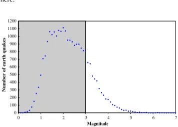
Earthquake magnitude distribution has been observed from the beginning of the 20th Century.Gutenberg and Richter (1942) and Ishimoto and Iida (1939) observed that the number of earthquakes,

N, of magnitude greater or equal toMfollows a power law distri-bution (seeFig. 1) defined by:

NðMÞ ¼

a

MB_{; ð1Þ}

where

a

andBare adjustment parameters.

Gutenberg and Richter (1954)transformed this power law into a linear law (seeFig. 2) expressing this relation for the magnitude frequency distribution of earthquakes as:

log10ðNðMÞÞ ¼abM: ð2Þ

This law relates the cumulative number of eventsN(M) with magni-tude greater or equal toMwith the seismic activity,a, and the size distribution factor,b. Thea-value is the logarithm of the number of earthquakes with magnitude greater or equal to zero. Theb-value is a parameter that reflects the tectonic of the area under analysis (Lee & Yang, 2006) and it has been related with the physical character-istics of the area. A high value of the parameter implies that the number of earthquakes of small magnitude is predominant and, therefore, the region has a low resistance. On the other hand, a low value shows that the relative number of small and large events is similar, implying a higher resistance of the material.

Gutenberg and Richter used the least squares method to esti-mate coefficients in the frequency–magnitude relation from(2). Shi and Bolt (1982)pointed out that theb-value can be obtained by this method but the presence of even a few large earthquakes has a significative influence on the results. The maximum likeli-hood method, hence, appears as an alternative to the least squares method, which produces estimates that are more robust when the number of infrequent large earthquakes changes. They also dem-onstrated that for large samples and low temporal variations of

b, the standard deviation of the estimatedbis:

rð

^_{bÞ ¼2:30b}2

rð

MÞ; ð3Þ where:

r

2_{ðMÞ ¼} Pn i¼1ðMiMÞ 2 n ð4Þ

andnis the number of events and Mithe magnitude of a single event.

It is assumed that the magnitudes of the earthquakes that occur in a region and in a certain period of time are independent and identically distributed variables that follow the Gutenberg–Richter law (Ranalli, 1969). This hypothesis is equivalent to suppose that the probability density of the magnitudeMis exponential:

fðM;bÞ ¼bexp½bðMM0Þ; ð5Þ

where

b¼ b

logðeÞ ð6Þ

andM0is the cutoff magnitude.

Thus, in order to estimate theb-value, a previous estimation of bis necessary. In Utsu (1965), the maximum likelihood method was applied to obtain a value forb, defined by:

b¼ 1

MM0

; ð7Þ

where M is the mean magnitude of all the earthquakes in the dataset.

From all the aforementioned possibilities, the maximum likeli-hood method has been selected for the estimation of theb-value in this work.

4.2. The b-value as seismic precursor

The b-value of the Gutenberg–Richter law is an important parameter, because it reflects the tectonics and geophysical prop-erties of the rocks and fluid pressure variations in the region con-cerned (Lee & Yang, 2006, Zollo, Marzocchi, Capuano, Lomaz, & Iannaccone, 2002). Thus, the analysis of its variation has often been used in earthquake prediction (Nuannin, Kulhanek, & Persson, 2005). It is important to know how the sequence ofb-values has been obtained, before presenting conclusions about its variation. The studies of bothGibowitz (1974) and Wiemer et al. (2002)on the variation of the b-value over time refer to aftershocks. They found an increase inb-value after large earthquakes in New Zea-land and a decrease before the next important aftershock. In gen-eral, they showed that theb-value tends to decrease when many earthquakes occur in a local area during a short period of time.

Other authors Schorlemmer, Wiemer, and Wyss (2005),

Nuannin et al. (2005)infer that theb-value is a stress meter that 0 100 200 300 400 500 600 700 800 900 1000 1100 1200 0 1 2 3 4 5 6 7 Magnitude

Number of earth quakes

Fig. 1.Number of earthquakes against magnitude (removing foreshocks and aftershocks) from the SGI database.

Magnitude

Fig. 2.Gutenberg–Richter law for the earthquakes (removing foreshocks and aftershocks) from the SGI database.

depends inversely on differential stress. Hence, Nuannin et al. (2005) presented a very detailed analysis on b-value variations. He studied the earthquakes in the Andaman–Sumatra region. To consider variations in b-value, a sliding time-window method was used. From the earthquake catalogue, theb-value was calcu-lated for a group of fifty events. Then the window was shifted by a time corresponding to five events. They conclude that earth-quakes are usually preceded by a large decrease inb, although in some cases a small increase in this value precedes the shock.

Sammonds, Meredith, and Main (1992) clarifies the stress changes in the fault and the variations of theb-value surrounding an important earthquake. They state: ‘‘A systematic study of tem-poral changes in seismic b-values has shown that large earth-quakes are often preceded by an intermediate-term increase inb, followed by a decrease in the months to weeks before the earth-quake. The onset of theb-value can precede earthquake occurrence by as much as seven years”.

5. Pattern recognition in seismic temporal data

The methodology proposed in order to discover knowledge from earthquakes time series is described in this section.

First of all, the earthquakes dataset is constructed as follows. Each earthquake is represented by three features: the magnitude, theb-value and the date of occurrence. Thus, theith earthquake is defined by:

Ei¼ ðMi;bi;tiÞ; ð8Þ

whereMiis the magnitude of the earthquake,biis theb-value asso-ciated to the earthquake andtiis the date in which the earthquake took place.

Theb-value is determined from(6) and (7)considering the fifty preceding eventsNuannin et al. (2005).Fig. 1illustrates that the number of earthquakes with magnitude greater or equal to three follows an exponential law allowing the application of the Guten-berg–Richter law from(5). Therefore, the cutoff magnitude is set to three.

Furthermore, data are grouped into sets of five chronologically ordered earthquakes according to the methodology proposed in Nuannin et al. (2005). Thus, a simpler law with easier interpreta-tion is provided. Each groupGjis represented by the mean of the magnitude of the five-earthquakes, the time elapsed from the first earthquake and the fifth one and the signed variation of theb -val-ues in this time interval, i.e.,

Gj¼ fEk4;. . .;Ekg withk¼5j and j¼1;. . .;bN=5c; ð9Þ

whereNis the number of earthquakes in the dataset andbN/5cis the greatest integer less than or equal toN/5. Thus,

Gj¼ ðMj;

D

bj;

D

tjÞ; ð10Þ where Mj¼ 1 5 Xk i¼k4 Mi; withk¼5j; ð11Þ

D

b¼bkbk4; withk¼5j; ð12Þ

D

tj¼tktk4; withk¼5j: ð13Þ

Finally, the dataset is composed by the temporal sequence of allGj,

DS¼ fG1;G2;. . .;GbN=5cg: ð14Þ

The goal is to find patterns in data that precede the apparition of earthquakes with a magnitude greater or equal to 4.5. Hence, the

K-means algorithm is applied to the dataset, DS, with the aim of classifying the samples into different groups. As a previous step, the optimal number of clusters has to be determined since theK

-means algorithm needs this number as input data. For this purpose, a well-known validity index – silhouette index – is applied over clustered data for different numbers of clusters. Thus, each sample is considered only by the label assigned by theK-means algorithm in further analysis. Once these labels have been obtained, specific sequences of labels are searched as precursors of medium–large earthquakes.

Sections5.1 and 5.2detail theK-means algorithm and the sil-houette index.

5.1. The K-means algorithm

TheK-means algorithm was originally presented byMacqueen (1968). For each cluster, its centroid is used as the most represen-tative point. The centroid of a group of elements is the center of gravity of all the elements in the cluster. Consequently, it can only be applied when the average of each cluster can be defined, i.e., the

K-means algorithm can classify datasets containing quantitative features.

The algorithm gathersnobjects intoKsets and increases the in-tra-cluster similarity at the same time. This similarity is measured with respect to the centroid of the objects that belong to the clus-ter. Then, the aim is to minimize intra-cluster variance defined as the following squared error function:

V¼X K i¼1 X xjCi jxj

l

ij 2 ; ð15Þ

whereKis the number of clusters,Ciis the clusteri,

li

is the cen-troid of the clusteriandxjis thej-thobject to be clustered.

TheK-means algorithm is an efficient and simple method espe-cially useful when large datasets are handled and it converges ex-tremely quick in most practical cases. In this work, K-means is applied several times in order to avoid that local minima are found and to reduce the dependency to the initial centers of clusters which are randomly selected.

5.2. Selecting the optimal number of clusters

The number of clusters selected to carry out classification is one of the most critical decisions in clustering techniques. Choosing a large number of clusters does not necessarily imply better classifi-cations. On the contrary, results could be unclear and confusing.

The selection of an optimal number of clusters is still an open task. Recently, several approaches have been developed in order to determine this number (Hamerly & Elkan, 2003; Yan & Ye, 2007) and its application has been shown to be useful in many engineering applications. In this sense, the silhouette index ( Kauf-mann & Rousseeuw, 1990) provides a measure of the separation of clusters and can be used as a general-purpose method to deter-mine the number of clusters.

Let be an objectxjthat belongs to clusterCi. The average dissim-ilarity ofxjto all the other objects included inCi,a(j), is evaluated as follows: aðjÞ ¼ 1 sizeðCiÞ X xi2Ci dðxi;xjÞ; withxi–xj; ð16Þ

whered(,) is a distance measure. Analogously, the average dissim-ilarity ofxjto all the objects belonging toCmwithm–iis called dis(xj,Cm) and defined by:

disðxj;CmÞ ¼minfdðxj;xlÞ;

8

l2Cmg; withm–i: ð17Þ

The next step consists in evaluating thedis(xj,Cm) for everym –i and, subsequently, the smallest dissimilarity is chosen as follows:

Thus,b(j) represents the dissimilarity ofxjto its nearest neighboring cluster. Finally, to determine how well an objectxjis clustered the following silhouette index is applied:

silhðjÞ ¼ bðjÞ aðjÞ

maxfaðjÞ;bðjÞg: ð19Þ

Its value ranges from1 to +1, where +1 and1 indicates points with adequate or questionable cluster assignment, respectively. If clusterCiis a set containing a single member, thensilh(j) is not de-fined and a conventional choice is to setsilh(j) = 0. The best cluster-ing is achieved when the average ofsilh(j) over thenobjects to be classified is maximized.

6. Experimental results

The patterns obtained by the application of theK-means algo-rithm to the seismic temporal data are presented in this section. First, the datasets used are detailed as well as the estimation of theb-value over these data. Second, the clustering process is de-scribed showing how the number of clusters is selected. Then, a measure of quality of the results is provided and a statistical anal-ysis is carried out with the aim of determining if the results ob-tained by the clustering are significative.

6.1. Dataset

The seismogenic areas used in this paper were established by Martín Martín (1989) according to tectonic, geological, seismic and gravimetric data. Twenty-seven areas are enumerated inTable 1.Fig. 3shows the epicenters of earthquakes localized in these 27 seismogenic areas from the year 1978. When the magnitude is greater or equal to 3.0 and less than 4.0 the epicenters are repre-sented by dots; when it is greater or equal to 4.0 and less than 5.0 the epicenters are marked with white circles; and finally, for earthquakes with magnitude greater or equal to 5.0, their epicen-ters are represented by black solid.

Foreshocks and aftershocks have been removed and only the earthquakes located between 35N to 44N and 10W to 5E have been selected. The samples include 4017 earthquakes, whose magnitude varies between 3.0 and 7.0, during the 29 year period from the year 1978 to the year 2007. Moreover, the catalogue is complete for earthquakes with magnitude greater or equal to 3.0 due to the year of completeness for the Spanish seismic data is the year 1978. At present, the proposed methodology has only been applied to the under-water seismogenic areas]26 and]27 (Alboran sea and Wes-tern Azores–Gibraltar fault, respectively) because there are not en-ough data in the remaining areas to carry out such an analysis. For both seismogenic areas, the maximum likelihood method has been used to obtain theb-value of the Gutenberg–Richter law. The cutoff magnitude is equal to three and theb-value is determined from(6) and (7) considering the fifty preceding events Nuannin et al. (2005).

6.2. Data clustering results

Fig. 4presents the mean of the silhouette index values versus the number of clusters for the seismogenic areas]26 and]27. It can be observed that the optimal number of clusters is three since the index reaches the maximum value for three clusters in both areas. Notice that the maximum values were equal to 0.6901 and 0.7532 for the areas]26 and]27, respectively, leading to a great accuracy.Fig. 5 shows the values of the silhouette index for all earthquakes from dataset which have been clustered. It can be noted an excellent adjustment of the data to the chosen number of clusters as nearly no negative values appear and the negative values indicate earthquakes with wrong cluster assignment.

Table 2shows the values of the centroids of the obtained clus-ters by using theK-means algorithm and the percentage of earth-quakes that belong to each cluster for seismogenic areas]26 and ]27. Once the earthquakes have been clustered, the values 1, 2 and 3 are the labels assigned to the different clusters. Notice that the majority of the earthquakes belong to the cluster one and three for the area]26 (34.38% and 56.24%, respectively). With reference to theb-value, clusters 1, 2 and 3 are characterized as follows. Clus-ter 1 presents a decrease of theb-value, cluster 2 an increment close to zero and, finally, cluster 3 an increase of theb-value. More-over, the magnitude of the centroid of the cluster 1 is greater to that of the cluster 2, and that of the cluster 2 is greater to that of the cluster 3 for both areas. In short, all earthquakes with magni-tude greater or equal to 4.5 have been classified into cluster 1 and characterized, therefore, by an increment of the b-value negative.

Figs. 6 and 7present the earthquakes temporal data,DS, classi-fied into 3 clusters along with the evolution of theb-value from the year 1978 to 2007. All the earthquakes of the dataset with magni-tude greater or equal to 4.5 are also represented by a black circle. Seismogenic area]26 is characterized by moderate seismicity with a Gutenberg–Richter b-value of 1.14 determined from (6) and (7)and a standard deviation of 0.05 obtained from(3). Analo-gously, the seismogenic area]27 presents a higher rate of large earthquakes with ab-value of 0.70 ± 0.03. In spite of the annual rate of earthquakes per square kilometer being similar in both areas (3.75E-04 in area]26 and 3.89E-04 in area]27), events of magnitude greater or equal to 4.5 are much more frequent in the West of Azores–Gibraltar fault than in the Alboran Sea. It is known that theb-value reflects the tectonics of the region under analysis (Lee & Yang, 2006) and, thus, a high value indicates that the rocks of the area have low strength and, consequently, the number of earthquakes with small magnitude is more frequent (Lowrie, 2007).

From Fig. 6, it can be observed that all the earthquakes of magnitude greater or equal to 4.5 (black circles) are preceded by Table 1

Seismogenic areas of Spain and Portugal. Area Description ]1 Granada basin ]2 Penibetic area

]3 Area to the East of the Betic system ]4 Quaternary Guadix–Baza basin

]5 Area of moderate seismicity to the North of the Betic system ]6 Area of moderate seismicity including the Valencia basin ]7 Sub-betic area

]8 Tertiary basin in the Guadalquivir depression ]9 Algarve area

]10 South-Portuguese unit ]11 Ossa Morena tectonic unit ]12 Lower Tagus Basin ]13 West Portuguese fringe ]14 North Portugal ]15 West Galicia ]16 East Galicia

]17 Iberian mountain mass ]18 West of the Pyrenees

]19 Mountain range of the coast of Catalonia ]20 Eastern Pyrenees

]21 Southern Pyrenees ]22 North Pyrenees ]23 North–Eastern Pyrenees

]24 Eastern part of Azores–Gibraltar fault ]25 North Morocco and Gibraltar field ]26 Alboran Sea

five-earthquake groups that belong to the cluster 3, except for one earthquake, occurred from the year 1993 to 1994, preceded by a five-earthquake group that belongs to the cluster 1. This only earthquake can be considered a separately case or an outlier for this area.

When the set of the preceding five-earthquakes was classified into cluster 3, the mean magnitude of this set is low and the incre-ment of theb-value is positive according to theTable 2. When an earthquake of magnitude greater or equal to 4.5 occur, the group of five-earthquakes including this large earthquake belongs to the cluster 1. Therefore, it can be noted that the sequence of labels that characterize the earthquakes with magnitude greater or equal to 4.5 for this area is 3–1. The change of the membership from clus-ter 3 to clusclus-ter 1 entails that theb-value decreases in a short time (from 1 to 2 months) nearby the occurrence of the shock (seeTable 2). Consequently, a decrease of theb-value is a precursor of earth-quakes of magnitude greater or equal to 4.5 for the area]26.

Fig. 3.Seismogenic areas of Spain and Portugal.

2 3 4 5 6 7 8 9 10 0.4 0.5 0.6 0.7 0.8 Number of clusters

Mean silhouette values

Zone 26 Zone 27

Fig. 4.Selection of the optimal number of clusters.

0 0.2 0.4 0.6 0.8 1 1 2 3 Silhouette Value Cluster −0.2 0 0.2 0.4 0.6 0.8 1 1 2 3 Silhouette Value Cluster

It can be observed that several five-earthquake groups with small magnitude are classified into the cluster 2, in which theb -va-lue is nearly constant and probably no important stress changes occur.

FromFig. 7, it can be stated that the seismogenic area]27 fol-lows a similar pattern to area]26 until the year 2000. That is, the membership of five-earthquake groups to clusters changes from cluster 3 to 1 when a moderate–large earthquake occurs. Around the year 2000, a period of great tectonic activity take place where many earthquakes of magnitude greater or equal to 4.5 are

recorded. This period is characterized by short time intervals in which five–earthquake groups change their membership from cluster 2 to 1, from cluster 1 to 2 and from cluster 1 to 1. However, all earthquakes of magnitude greater or equal to 4.5 (black circles) are classified into cluster 1 and most of them are preceded by five– earthquake groups that belong to the cluster 2 or 1 (sequences of labels 2–1 and 1–1). It can be observed that most of preceding earthquakes classified into cluster 1 are, at the same time, pre-ceded by earthquakes that belong to the cluster 2. Let be 1–12

the subset of earthquakes classified into the cluster 1 and preceded by earthquakes belonging to the cluster 1 that are preceded by earthquakes classified into the cluster 2. Moreover, three earth-quakes with magnitude greater or equal to 4.5 classified into clus-ter 1 also appeared in the last quarclus-ter of the year 2006. However, the preceding five-earthquake groups are not classified into the cluster 2 but into the cluster 3, in contrast to what it happens in the 1–12_{sequence. This sequence is denoted by 1–1}3_{. Therefore,}

the sequences that characterize the earthquakes with magnitude greater or equal to 4.5 for the area]27 are 2–1, 1–12_{and 1–1}3_.

Thus, a decrease of theb-value is considered a precursor of moderate–large earthquakes for this area due to the change of Table 2

Centroids of the clusters.

Area Cluster M Db Dt Membership (%) ]26 ]1 3.56 0.047 0.16 34.38 ]2 3.39 0.013 0.83 9.38 ]3 3.28 +0.028 0.16 56.24 ]27 ]1 3.99 0.028 0.140 34.62 ]2 3.54 0.005 0.091 43.59 ]3 3.33 +0.035 0.519 21.79

Fig. 6.Clustering of earthquakes for the Alboran sea.

membership of preceding earthquakes from cluster 3 to 1 in the se-quence 1–13_{and from cluster 2 to 1 in the sequences 1–1}2_{and 2–1}

(seeTable 2).

Moreover, it can be noticed that several earthquakes with small magnitude, occurring before the year 1995 with a longer period of time among them, are classified into cluster 3 implying a large in-crease of theb-value.

In short, when a group of small earthquakes is classified into the cluster 3 or 2 and theb-value begins to decrease, the occurrence of an earthquake with magnitude greater or equal to 4.5 in a near fu-ture is forecasted and furthermore, this large earthquake will be classified into the cluster 1.

6.3. Quality of the results

All earthquakes with a magnitude greater or equal to 4.5 are classified into cluster 1 and most of these earthquakes were pre-ceded by others belonging to cluster 3, cluster 2, sequence of clus-ters 2–1 or sequence of clusclus-ters 3–1. Therefore, the sequences of labels 3–1, 2–1, 1–12_{and 1–1}3_{are now going to be studied in order}

to provide a measure of the quality of the obtained results in the previous subsection.

Table 3provides the distribution of all earthquakes for different clusters taking into consideration the cluster in which the preced-ing earthquakes are classified. The Hits columns identify those earthquakes that have magnitudes greater or equal to 4.5. It can stated that most of Hitsare represented by sequences of labels 3–1, 2–1 and 1–12_{(13, 9 and 7, respectively).}

The last column makes reference to the existing ratio between the number of earthquakes with magnitude greater or equal to 4.5 classified into each sequence and the total occurrences of such sequence. Note that the ratio corresponding to the sequences 3–1, 2–1 and 1–12_{are 0.65, 0.56 and 1, respectively. These values are}

the highest ones among that of all sequences except for the se-quence 1–13_{, which has a similar ratio to the ones in sequences}

3–1 and 2–1 (0.60 versus 0.65 and 0.56, respectively). Thus, the se-quence 1–13_{is also considered to be representative, as it was}

sta-ted in the previous section.

True positives (TP) identify the occurrence of earthquakes with magnitude greater or equal to 4.5 when any of the considered se-quences of labels are present. On the other hand, the false nega-tives (FN) represent the number of cases in which a medium– large earthquake also occurs but no proposed sequences of labels are found. True negatives (TN) and false positives (FP) refer to the situation in which no earthquakes occurred. However, the TN denotes that no proposed sequences appear, while the FP makes reference to the apparition of any of the considered sequences.

In addition, two well-known indices are provided, the sensitiv-ity and the specificsensitiv-ity. In this context, the sensitivsensitiv-ity quantifies the

grade of reliability of the method when real events take place while the specificity measures the reliability of the method when sequences of labels are discarded. These indices are defined by the following equations:

Sensitivity¼ TP

TPþFN; ð20Þ

Specificity¼ TN

FPþTN: ð21Þ

Table 4measures the quality of the results obtained from the earth-quakes temporal data distribution shown inTable 3. It can be ob-served that the method obtains good levels of accuracy, since sensitivities of 90.00% and 79.31% are reached for areas #26 and #27, respectively. Furthermore, the specificity reaches values great-er than 80% and 90% for the areas #26 and #27, respectively. In short, not only medium–large earthquakes are detected with a good reli-ability, but also those cases in which earthquakes with a magnitude lesser than 4.5 appear are properly discarded. The obtained perfor-mance is considered relevant for geophysical data analysts as the occurrences of earthquakes present a high level of uncertainty.

6.4. Statistical analysis

The well-known Wilcoxon rank-sum (WRS) test is applied in or-der to show that the magnitude distributions of the earthquakes that belong to the sequences 3–1, 2–1, 1–13and 1–12come from the same distribution with equal medians. The test has been ap-plied to all possible two–sequence combinations.

The WRS is a standard non–parametric test for two independent samples based on data ranking and it has been chosen because the required conditions to apply parametric tests, such as normality of data, are not satisfied. A null hypothesis is an assumption about the population to be tested. This hypothesis is accepted or rejected by the test according to thep-value. When thep-value is lesser or greater than a certain level of significance the hypothesis is re-jected or accepted, respectively. Therefore, the level of significance is the probability of rejecting the null hypothesis being true. For in-stance, when the level of significance is 0.05, the probability of making a mistake rejecting the null hypothesis is 5%.

In this context, the samples are the maximum magnitudes of the groups of five-earthquakes classified into the cluster 1 for all sequences of clusters 3–1, 2–1, 1–13and 1–12versus the remaining sequences of two clusters. Therefore, the null hypothesis assumes that these magnitudes are equally likely to occur. The level of sig-nificance has been set to 0.05 as it is considered a typical level of significance in most of statistical tests. The test has been applied to the joining of all samples from both areas #26 and #27 since the number of the earthquakes classified into some of the se-quences 3–1, 2–1, 1–13_{and 1–1}2_{is not representatively enough}

for both areas separately. For instance, the sequence of labels 2– 1 only appears twice in area #26 and the sequence 3–1 only ap-pears three times in area #27.

Table 5shows thep-values obtained by the application of the WRS test to the samples for seismogenic areas #26 and #27, where the number in brackets represents the number of occurrences of Table 3

Distribution of earthquakes into different sequences.

Sequences Area #26 Area #27 Ratio

Cases Hits Cases Hits 1–11 7 1 3 3 0.40 1–12 1 0 6 7 1 1–13 4 0 1 3 0.60 1–2 1 0 14 0 0 1–3 16 0 2 0 0 2–1 2 0 14 9 0.56 2–2 2 0 16 2 0.11 2–3 5 0 4 1 0.11 3–1 17 9 3 4 0.65 3–2 6 0 4 0 0 3–3 35 0 10 0 0 Total 96 10 77 29 Table 4 Results performance.

Parameters Area #26 Area #27

TP 9 23 FN 1 6 FP 15 5 TN 71 47 Sensitivity 90.00% 79.31% Specificity 82.56% 90.38%

each sequence of clusters for areas #26 and #27, respectively. The sequence 1–11is the subset of earthquakes classified into the clus-ter 1 and preceded by earthquakes belonging to the clusclus-ter 1 that are preceded by earthquakes classified into the cluster 1 at the same time. The last column provides the mean of the samples cor-responding to each sequence of clusters. It can be noticed that the average magnitudes of the earthquakes classified into the se-quences of clusters 3–1, 2–1 and 1–12 _{are higher than those of}

other sequences (greater or equal to 4.5, concretely).

Moreover, the p-values obtained for the samples of the se-quences 3–1, 2–1, 1–13_{and 1–1}2_{are greater than 0.05. Therefore,}

the null hypothesis cannot be rejected and the distributions of earthquakes that belong to these sequences are the same, accord-ing to their magnitude. The null hypothesis cannot be either re-jected for the sample corresponding to the sequence 1–11 since the values provided by the WRS test are higher than 0.05. Never-theless, the number of earthquakes with a magnitude greater or equal to 4.5 that are classified in this sequence is low regarding the total occurrences of this sequence (a ratio of 0.4, concretely) but these earthquakes have magnitudes specially high, leading to a mean magnitude equal to 4.4, very close to the considered threshold.

The null hypothesis for the remaining sequences is rejected since thep-values are lesser than 0.05 and 0 in many cases. This means that the magnitudes of the earthquakes classified into se-quences of clusters 1–2, 1–3, 2–2, 2–3, 3–2 and 3–3 have a distri-bution different to those of the sequences 3–1, 2–1, 1–13_{and 1–1}2_.

In short, the sequences of clusters 3–1, 2–1, 1–13and 1–12are sig-nificant sequences to discover patterns as precursors of moderate– large earthquakes.

7. Conclusions

In this paper a pattern recognition based onK-means algorithm is proposed to forecast earthquakes with magnitude greater or equal to 4.5. Results corresponding to the Spanish seismic temporal data provided by the Spanish Geographical Institute are reported, yielding a sensitivity and a specificity which are 90.00% and 82.56% in area #26 and 79.31% and 90.38% in area #27. Moreover, all medium–large earthquakes have been characterized by a decre-ment of theb-value. Thus, this parameter can be considered a seis-mic precursor for the Spanish seisseis-mic data. It can be stated that the

K-means approach has a good performance, particularly when the uncertainty of earthquakes occurrences is taken into account. Acknowledgements

The financial support given by the Spanish Ministry of Science and Technology, projects BIA2004-01302 and TIN-68084-C02 and by the Junta de Andalucía, project P07-TIC-02611 is acknowledged.

References

Bird, P., & Liu, Z. (2007). Seismic hazard inferred from tectonics: California. Seismological Research Letters, 78(1), 37–48.

Ebel, J. E., Chambers, D. W., Kafka, A. L., & Baglivo, J. A. (2007). Non-poissonian earthquake clustering and the hidden Markov model as bases for earthquake forecasting in California.Seismological Research Letters, 78(1), 57–65. Field, E. H. (2007). Overview of the working group for the development of regional

earthquake likelihood models (RELM). Seismological Research Letters, 78(1), 7–16.

Frankel, A. D., Petersen, M. D., Mueller, C. S., Haller, K. M., Wheeler, R. L., & Leyendecker, E. V. et al. (2002).Documentation for the 2002 update of the national seismic hazard map. Technical Report 02-420. United States Geological Survey. Geller, R. J. (1997). Earthquake prediction: A critical review.Geophysical Journal

International, 131(3), 425–450.

Gerstenberguer, M. C., Jones, L. M., & Wiemer, S. (2007). Short-term aftershock probabilities: Case studies in California.Seismological Research Letters, 78(1), 66–77.

Gibowitz, S. J. (1974). Frequency–magnitude depth and time relations for earthquakes in Island Arc: North Island, New Zealand.Tectonophysics, 23(3), 283–297.

Giner, J. J., Molina, S., Jauregui, P., & Delgado, J. (2002). A new methodology for decreasing uncertainties in the seismic hazard assesment results by using sensitivity analysis. An application to sites in Eastern Spain.Pure and Applied Geophysics, 159, 1271–1288.

Gutenberg, B., & Richter, C. F. (1942). Earthquake magnitude, intensity, energy and acceleration.Bulletin of the Seismological Society of America, 32(3), 163–191. Gutenberg, B., & Richter, C. F. (1954).Seismicity of the Earth. Princeton University. Hamerly, G. & Elkan, C. (2003). Learning thekink-means. InProceedings of the

Seventeenth Annual Conference on Neural Information Processing Systems(pp. 281–288).

Helmstetter, A., Kagan, Y. Y., & Jackson, D. D. (2007). High-resolution time-independent grid-based forecast for M = 5 earthquakes in California. Seismological Research Letters, 78(1), 78–86.

Holliday, J. R., Chen, C. C., Tiempo, K. F., Rundle, J. B., Turcotte, D. L., & Donnellan, A. (2007). A RELM earthquake forecast based on pattern informatics.Seismological Research Letters, 78(1), 87–93.

Ishimoto, M., & Iida, K. (1939). Observations sur les seismes enregistres par le microsismographe construit derniereme.Bulletin Earthquake Research Institute, 17, 443–478.

Justo Alpañés, J. L., Carrasco, R. & Martín Martín, A. J. (1999). The seismogenetic zones and magnitude–frequency relationship of Andalusian region. In Proceedings of International Conference on Earthquake Geotechnical Engineering (pp. 175–179).

Kafka, A. L., & Levin, S. Z. (2000). Does the spatial distribution of smaller earthquakes delineate areas where larger earthquakes are likely to occur?Bulletin of the Seismological Society of America, 90, 724–738.

Kagan, Y. Y., & Jackson, D. D. (1994). Long-term probabilistic forecasting of earthquakes.Journal of Geophysical Research, 99(13), 685–700.

Kagan, Y. Y., Jackson, D. D., & Rong, Y. (2007). A testable five-year forecast of moderate and large earthquakes in Southern California based on smoothed seismicity.Seismological Research Letters, 78(1), 94–98.

Kaufmann, L., & Rousseeuw, P. J. (1990).Finding groups in data: An introduction to cluster analysis. John Wiley & Sons.

Kulhanek, O. (2005). Seminar on b-value. Technical report. Department of Geophysics, Charles University, Prague.

Lee, W. H. K., Bennet, R. E, & Meagher, K. L. (1972).A method of estimating magnitude of local earthquakes from signal duration. Technical Report 72-223, United States Geological Survey.

Lee, K., & Yang, W. S. (2006). Historical seismicity of Korea. Bulletin of the Seismological Society of America, 71(3), 846–855.

López, C., & Muñoz, D. (2003). Magnitude formulas in the Spanish bulletins and catalogues.Física de la Tierra, 15, 49–71 (in Spanish).

Lowrie, W. (2007).Fundamentals of Geophysical. Cambridge University Press. Macqueen, J. B. (1968). Some methods for classification and analysis of multivariate

observations. InProceedings of the 5th Berkeley symposium on mathematical statistics and probability(pp. 281–297).

Martínez-Álvarez, F., Troncoso, A., Riquelme, J. C., Riquelme, J. M. (2007). Partitioning–clustering techniques applied to the electricity price time series. InLecture Notes in Computer Science(pp. 990–991).

Martín Martín, A. J. (1989). Probabilistic seismic hazard analysis and damage assessment in Andalusia (Spain).Tectonophysics, 167, 235–244.

Mezcua, J., Rueda, J., & García Blanco, R. M. (2004). Reevaluation of historic earthquakes in Spain.Seismological Research Letters, 75(1), 189–204. Murru, M., Console, R., & Falcone, G. (2009). Real time earthquake forecasting in

Italy.Tectonophysics, 470(3–4), 214–223.

Nuannin, P., Kulhanek, O., & Persson, L. (2005). Spatial and temporal b-value anomalies preceding the devastating off coast of NW Sumatra earthquake of December 26, 2004.Geophysical Research Letters, 32.

Petersen, M. D., Cao, T., Campbell, K. W., & Frankel, A. D. (2007). Time-independent and time-dependent seismic hazard assessment for the state of California: Uniform California earthquake rupture forecast model 1.0. Seismological Research Letters, 78(1), 99–109.

Ranalli, G. (1969). A statistical study of aftershock sequences.Annali di Geofisica, 22, 359–397.

Table 5

p-values for the WRS test.

Shifts 3–1 2–1 1–13 1–12 Mean 1–11 (7/3) 0.648 0.542 0.867 0.168 4.4 1–12 (1/6) 0.363 0.365 0.219 1.000 4.8 1–13_{(4/1) 0.376 0.507 1.000 0.134 4.4} 1–2 (1/14) 0.013 0.005 0.023 0.005 4.0 1–3 (16/2) 0.000 0.000 0.000 0.000 3.5 2–1 (2/14) 1.000 1.000 0.814 0.365 4.6 2–2 (2/16) 0.004 0.003 0.035 0.003 4.0 2–3 (5/4) 0.002 0.000 0.013 0.002 3.8 3–1 (17/3) 1.000 0.898 0.376 0.390 4.6 3–2 (6/4) 0.001 0.000 0.005 0.000 3.8 3–3 (35/10) 0.000 0.000 0.000 0.000 3.7

Rhoades, D. A. (2007). Application of the EEPAS model to forecasting earthquakes of moderate magnitude in Southern California. Seismological Research Letters, 78(1), 110–115.

Sammonds, P. R., Meredith, P. G., & Main, I. G. (1992). Role of pore fluid in the generation of seismic precursors to shear fracture.Nature, 359, 228–230. Schorlemmer, D. G., Wiemer, S., & Wyss, M. (2005). Variations in earthquake-size

distribution across different stress regimes.Nature, 437(7058), 539–542. Sfetsos, A., & Siriopoulos, C. (2004). Combinational time series forecasting based on

clustering algorithms and neural networks.Neural Computing and Applications, 13(1), 56–64.

Shen, Z. Z., Jackson, D. D., & Kagan, Y. Y. (2007). Implications of geodetic strain rate for future earthquakes, with a five-year forecast of M5 earthquakes in Southern California.Seismological Research Letters, 78(1), 116–120.

Shi, Y., & Bolt, B. A. (1982). The standard error of the magnitude–frequencyb-value. Bulletin of the Seismological Society of America, 72(5), 1677–1687.

Tsumura, K. (1967). Determination of earthquake magnitude from total duration of oscillation.Bulletin Earthquake Research Institute, 45, 7–18.

Utsu, T. (1965). A method for determining the value ofbin a formula log n = a-bm showing the magnitude–frequency relation for earthquakes. Geophysical bulletin of Hokkaido University, 13, 99–103.

Ward, S. N. (2000). San Francisco bay area earthquake simulations: A step toward a standard physical earthquake model. Bulletin of the Seismological Society of America, 90, 370–386.

Ward, S. N. (2007). Methods for evaluating earthquake potential and likelihood in and around California.Seismological Research Letters, 78(1), 121–133. Wiemer, S., Gerstenberger, M., & Hauksson, E. (2002). Properties of the aftershock

sequence of the 1999 Mw 7.1 hector mine earthquake: Implications for aftershock hazard. Bulletin of the Seismological Society of America, 92(4), 1227–1240.

Wiemer, S., & Schorlemmer, D. (2007). ALM: An asperity-based likelihood model for California.Seismological Research Letters, 78(1), 134–143.

Xu, R., & Wunsch, D. C. II, (2005). Survey of clustering algorithms.IEEE Transactions on Neural Networks, 16(3), 645–678.

Yan, M., & Ye, K. (2007). Determining the number of clusters using the weighted gap statistic.Biometrics, 63(4), 1031–1037.

Zollo, A., Marzocchi, W., Capuano, P., Lomaz, A., & Iannaccone, G. (2002). Space and time behavior of seismic activity at Mt. Vesuvius volcano, Southern Italy. Bulletin of the Seismological Society of America, 92(2), 625–640.