Further investigations into the term structure of interest rates

(1)

Further Investigations into the Term

Structure of Interest Rates

Michael J. Howell

CrossBorder Capital Ltd. and Birkbeck College, University of London

(2)

Preface

I hereby declare that this thesis is my own work and includes nothing which is derived from collaboration; is not substantially the same as any other work I have submitted or will be submitting for a degree, diploma or other qualification, at this or any other university, and does not exceed the prescribed limit of 100,000 words.

I acknowledge than an earlier version of chapter 3 was published in the Journal of Investing, Fall 2014, Vol. 23, No. 3: pp. 86-97, under the title ‘Style Selection and US Investors’ Risk Appetite’ with co-author Dr. Hari P. Krishnan

Michael J. Howell April 2017

(3)

Abstract

Recent empirical term structure literature questions the usefulness of the standard three-parameter yield curve model in the wake of the Global Financial Crisis and the widespread adoption of unconventional monetary policies, such as Large-scale Asset Purchases (LSAP). This thesis builds on these concerns by extracting a new parameter from the term structure that measures the position of the traditional hump in the yield curve along the maturity axis. My alternative decomposition of the term structure makes it easier to track-down the influence of quantities on interest rates. Given that Treasuries are held as safe assets by many investor types, I interpret the new parameter as a gauge of investors’ risk appetite. It is time-varying and pro-cyclical, leading the business cycle and indexes of financial stress by several months and forming part of the risk-taking policy transmission channel. My results contradict the widely-held view from event studies that LSAP reduce long-term Treasury yields. They can also explain the often divergent relative movements between Treasury term premia and the premia on risky assets, such as corporate credits.

(4)

Acknowledgements

I offer thanks to my supervisors Pavol Povala, David Schroeder and Roald Versteeg, who have supported me in my research for this Phd, and to Ron Smith of Birkbeck College, who provided sound guidance and encouragement throughout. Stephen Wright gave additional helpful comments. I would also like to acknowledge Marty Leibowitz, formerly of Salomon Bros Inc. and now of Morgan Stanley Inc. in New York, for stimulating my original interest in fixed income markets and bond duration.

(5)

Summary

Further Investigations into the Term Structure of Interest Rates

Michael J. Howell

The interest rate term structure plays a critical role in the Neo-classical economic framework by linking together the present and the future. Applying latest mathematical and statistical techniques, the empirical literature increasingly acknowledges that it is no longer sufficient to characterise the term structure using just the standard three yield curve parameters of level, curvature and slope. In this PhD thesis, I seek to extract further information and add to existing knowledge by identifying and interpreting, to ensure is does not appear ad hoc, a fourth yield curve parameter, which ultimately may help to better understand the risk-taking policy transmission channel. This new parameter describes the position of the traditional hump in the yield curve along the maturity axis. Its existence has been previously recognised, but it is typically either discarded as having no economic meaning or else treated as a constant to simplify yield curve estimation. I argue here that the position of the hump contains valuable information about the risk appetite of economic agents, such as investors and credit-providers, largely because Treasury bonds represent canonical safe assets. The greater demand for safety at longer investment horizons will reduce term premia at those tenors, causing the yield curve to flatten and the position of the hump to move inwards. The position of the hump could be measured from the degree of asymmetry implicit in the pattern of term premia across the Treasury term structure. But in practice, given the absence of reliable term premia estimates, I measure the position of the hump from spot yields using a statistic I create and name D-star (for ‘distance’). A higher (lower) D-star should capture the existence of negative (positive) skew in the pattern of term premia across the yield curve; so reflect excess supply (demand) for safe assets at longer tenors and, thus, signal risk-seeking (risk-avoiding) behaviour.

By including D-star, this new yield curve decomposition makes it easier to track down the influence of quantities on the shape of the term structure. I test whether empirical

(6)

estimates of D-star derived from the US Treasury market can predict future outcomes of a number of key macro-finance variables, notably the national financial stress indexes (FSIs), devised by various US Federal Reserve districts. It appears from my results that D-star consistently adds value around a year ahead. This suggests that D-star could be included among the array of variables regularly monitored for financial stability purposes. I subsequently proceed, in the final section of this thesis, to use these D-star estimates empirically to better understand policy transmission in the wake of the 2007/08 Global Financial Crisis and Great Recession (GFC) and the subsequent Large-scale Asset Purchases (LSAP) policy response. LSAP should cause D-star to fall-back alongside declining term premia, as is apparently shown by a large number of recent event studies. Paradoxically, I demonstrate the opposite result: LSAP policies ultimately have a positive effect on risk appetite and lengthen D-star. This, I argue, is because LSAP are multi-faceted: the signalling and liquidity impacts of LSAP on the demand for government bonds outweigh any scarcity and duration effects. Tracing thought the transmission channels using a Bayesian vector auto-regression (BVAR) model, these positive effects appear to be encouraged by second-round influences based on lower perceived systemic risks, explained by Treasuries being held as safe assets by many investors. In other words, the cash injections that are associated with a decrease in the effective supply curve for maturity subsequently induce an offsetting fall in the demand curve. Using this risk-taking transmission channel, I argue that LSAP ultimately result in higher (not lower) Treasury term premia, steeper (not flatter) yield curves and higher (not lower) long-term yields. My framework also helps to understand the apparent negative correlation between corporate debt spreads and Treasury term premia, because risk-seeking investors switch from safe to more risky assets. This outturn is time consistent with policy-makers’ original intentions to encourage greater risk-taking following the GFC. My empirical results suggest that changing risk appetite has the greater impact on corporate credit spreads, whereas the liquidity effect from LSAP is a more important determinant of Treasury term premia. The existence and measurement of D-star facilitate this re-interpretation.

Supervisors: Dr. David Schroeder/ Dr. Roald Versteeg

(7)

List of Tables

3.1 Cross-Correlation Coefficients between Yield Curve Factors, 1987-2016 ... 20

3.2 Cross-correlations (15 months ahead) and Granger Causality Tests (12 months) between US Financial Stress Index and High Yield Spread with various Yield Curve Factors, 1987-2016 ... 21

3.3 Summary Statistics – Various Estimates D-Star, 1946-2016 ... 40

3.4 Correlation Coefficients –Estimates D-Star and D-Peak, 1989-2016 ... 42

3.5 US Treasury Yield Curve Classified by Slope, Curvature and D-star, 1946-2017 ... 43

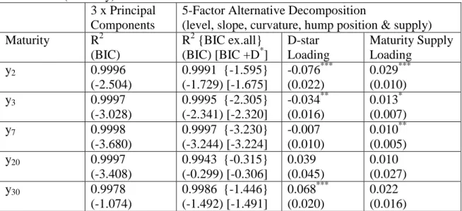
3.6 Regression of Selected US Treasury Yields on Various Yield Curve Factors, 1954-2016 ... 47

4.7 Granger Causality Tests – Summary Results ... 73

4.8 Regression of First Principal Component of Major US National Financial Stress Indexes on Principal Components of the US Treasury Yield Curve, with and without D-star, for various lead-times (3, 6, 9, 12, 15 and 18 months), 1994-2016 ... 75

(10)

List of Figures

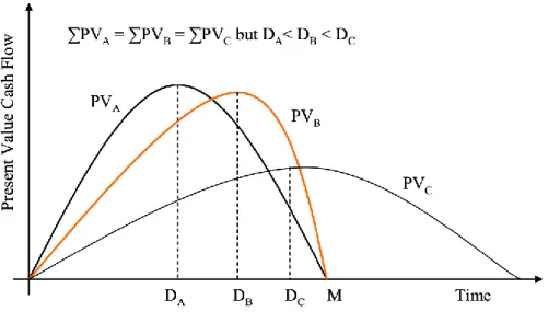
2.1 PresentValue Cash Flow Profiles of Three Assets and Their Duration ... 13

3.2 D-Star (Position of Curvature Peak in Years, 6-month CMA, Advanced 15 months and Inverted) and B-BBB Corporate Credit Spread, 1987-2016 ... 23

3.3 Liability Duration and Fixed Income Portfolio Duration – Sample of Major US Pension Funds, 2011-16 ... 30

3.4 The Average Maturity of US Treasury Securities Outstanding, 1946-2016; the Average Maturity of Federal Reserve Holdings, 2003-16 and Duration of Aggregate US Treasury Bond Index, 1980-16 ... 32

3.5 Yield Curve – Level, Slope, Curvature and Position ... 34

3.6 Maturity of Average Curvature (D-star) – Security-level and Generic US Treasury Yields, 1989-2016 ... 41

3.7 D-star(6-month CMA) and Yield Curve Slope (10-1 year), 1946-2016 ... 44

3.8 D-star(6-month CMA) and Curvature (10-5-1 year), 1946-2016 ... 45

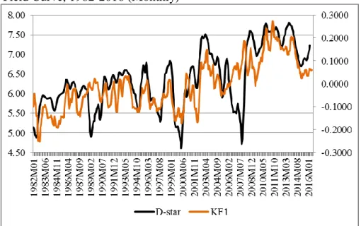
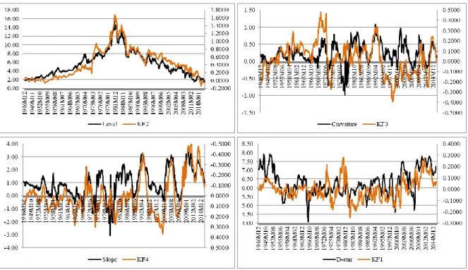
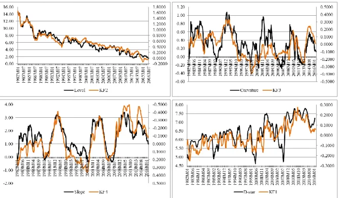
3.9 D-star (6-month CMA) and a Fourth Kalman Factor Filtered from Affine Yield Curve, 1982-2016 ... 49

4.10 First Principal Component of Major Financial Stress Indexes (FSIs), 1994-2016 ... 76

4.11 US Corporate Spreads, 1987-2016 ... 77

4.12 Financial Stress Indexes (FSIs) and Bond Risks, 1994-2016 ... 78

4.13 University of Michigan US Consumer Sentiment Survey, 1985-2016 ... 78

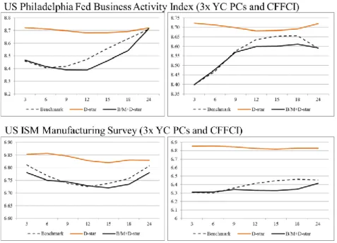
4.14 US Business Activity, 1954-2016 ... 80

4.15 USM Index 1954-2016 and 2000-2016 ... 80

4.16 BIC Tests on Risk Appetite Using Three Benchmarks, various time periods ... 81

4.17 US High Yield Spread (B-Baa) – Actual and Out-of-Sample Forecasts, 2004-16... 84

4.18 US Consumer Sentiment (University of Michigan) – Actual 12 month change and Out-of-Sample Forecasts, 2004-16 ... 84

4.19 Global Risk Appetite (ECB Measure) and D-star (inverted, advanced 12 months), 2006-2010 ... 85

4.20 Y2K Bubble Finance Crisis – D-star (Advanced) and Selected Macro-Finance Variables, 1999-2003 ... 86

4.21 Global Finance Crisis – D-star (Advanced) and Selected Macro-Finance Variables, 2006-10 ... 87

5.22 US QE Periods, Nominal Term Premia and 10-Year Treasury Yield, 2007-15 ... 98

(11)

5.24 US Corporate Credit Risk Premia (Junk CCC less High Yield Single B and High

Yield (B) less Investment Grade (BBB)) and LSAP Announcement Effects, 2008-2012 .... 101 5.25 D-star (Implied Risk Appetite) and LSAP, 2007-16 ... 114 5.26 Selected Impulse Response Functions ... 117 5.27 The Risk-Seeking Channel (Schematic) ... 119 5.28 Comparative Impulse Responses to D-star and Liquidity Shocks – 10-year

Treasury Term Premia and B-BBB Credit Spreads ... 121 5.29 Robustness Tests – Effects on IRFs of Dropping Lags and Restricting Sample Size ... 123

(12)

Chapter 1

Introduction: The Interest Rate Term Structure

“…yield quotations must appear as a bewildering welter of unrelated interest rates. Yet

this seeming jumble of rates is not without order.” Jacob B. Michaelsen, The Term

Structure of Interest Rates (1973)

The recent Global Financial Crisis and Great Recession (GFC) have focussed attention on the stability of the balance sheet structures of investors; the efficacy of subsequent zero-interest rate policy response (ZIPR) and the implementation and transmission of Large-scale Asset Purchases (LSAP). This thesis analyses the US Treasury interest rate term structure in this light. The term structure is central to the Neo-classical economic framework by linking the present with the future. It is traditionally characterised just by its level, slope and curvature. However, I identify a fourth parameter, based on the position of the hump in the yield curve along the maturity dimension, which adds new information and makes it easier to track down the influence of quantities on the shape of the term structure.

My starting point is an attempt to devise a practical measure of the implicit distribution of term premia across the Treasury term structure based on its degree of asymmetry. The position of the traditional hump in the yield curve along the maturity axis (i.e. the additional parameter) should characterise the distribution of term premia across tenors. I term this new parameter, D-star, and show that it can be easily calculated for all yield curve types using a simple distance measure. D-star estimates for the US are later cross-checked with a Kalman filtered factor. Although it is statistically significant, D-star does not add much in economic terms to the explanation of the current yield curve beyond that already known from the three traditional yield curve factors. However, it contains other information about the risk appetite of investors, which is relevant for the predictability of future yields. In fact, the general existence of unspanned macro-factors

(13)

that improve prediction has been studied by Coroneo et al. (2016). My approach differs because I argue that D-star also helps to forecast broader macro-finance variables, such as a composite US financial stress index (FSI) and the high yield credit spread (B less BBB-rated corporate bonds), approximately one year ahead. My results demonstrate significant one-way Granger causality for this new parameter, compared to the other yield curve factors. I go on to show that D-star allows a better understanding of the policy transmission mechanism, given the low importance assigned by Bernanke and Blinder (1992) to interest rates, and its existence enables us to more clearly delineate the

risk-taking channel from the credit channel.

It seems plausible that more distant (nearer) yield peaks in the term structure reflect relatively larger term premia at longer (shorter) time horizons. Intuitively, these should identify risk-seeking behaviour, because the demand for Treasury securities is a derived-demand for safe assets by many investor types. Safety is here defined in terms of a preferred habitat, based either on regulation needs or on duration and minimum liquidity requirements. Excess safe asset supply (demand) at any maturity will raise (lower) local term premia, resulting in limits to arbitrage. Hence, risk-seeking (avoiding) behaviour should lead to an excess supply of (demand for) Treasuries at longer horizons and so raise (depress) more distant term premia, causing a steeper (flatter) yield curve; a negatively (positively) skewed distribution of term premia and a yield curve hump positioned at a longer (shorter) tenor.

Recent large-scale asset purchases (LSAP) by Central Banks, in the wake of the 2007/08 Global Financial Crisis and Great Recession (GFC), and the growing safe asset demands from foreigners and domestic financial institutions, following new regulations, have disrupted the normal balance between supply and demand in the US Treasury markets. The effects of these quantitative imbalances, which are absent from the standard finance models, are likely to be felt across the interest rate term structure. When changes to the effective supply of government securities (including LSAP) distort local term premia, these scarcity effects may simply inconvenience certain investors and have a limited macro-economic impact beyond lowering average term premia and, hence, average Treasury yields. However, when these imbalances are driven by demand

(14)

factors, they may tell us something about investors’ risk appetites. I treat this as an empirical question, albeit one also faced when interpreting the standard yield curve factors. One complication is that changes in the authorities’ net supply function may themselves induce fluctuations in the demand functions of investors because they potentially signal future policy intentions (‘Forward Guidance’) as well as providing extra liquidity (‘Quantitative Easing’). Taken together these responses may reduce perceived systemic risks1.

A proper evaluation of these effects is made difficult because of a lack of data on the supply of bonds and investor demands across the various maturities and the widespread scarcity of reliable term premia data. These observations motivate the three core chapters of this thesis. These try to extract further quantitative information from the term structure, with a focus on implementing a practical estimation method for D-star, and then applying it to predict future financial stress and better understand the transmission of monetary policy. My key contributions in this thesis are:

 Measurement: The third chapter A New ‘Preferred Habitat’ Yield Curve

Parameter introduces a measure of the position of the traditional hump along the

maturity axis, termed D-star, that implicitly describes the cross-sectional pattern of term premia across tenors. This may also be the point where the curvature of the term structure peaks. Term premia are by implication relatively smaller at subsequent maturities. I use the preferred habitat framework of Vayanos and Vila (2009) and adapt the ‘gap filling’ model of Greenwood, Hanson and Stein (2010) to explain D-star. Low Treasury term premia at longer maturities suggest a smaller D-star value. This could reflect an excess demand for safety at those tenors, implying a reduced risk appetite among investors. Investors’ risk appetite is here defined in terms of deviations away from a risk-neutral duration point and calculated from the inflection point on the yield curve using a standard average distance measure. It might be described by market participants as the

1

It could be argued from a supply perspective that any lengthening in the average maturity of government debt, by postponing the need for subsequent re-financing, also reduces systemic risks.

(15)

‘duration-weighted average butterfly spread across tenors’. I explicitly do not use term premia estimates for this calculation. The derived factor represents a fourth yield curve parameter and is a convenient measure of the investment time horizon. The values of D-star are cross-checked with alternative Kalman filter estimates. The resulting data are time-varying, with a mean of 6.3 years (1946-2016) and a standard deviation of 10-months.

 Evaluation: Chapter 4 Using the Interest Rate Term Structure to Model Risk

Seeking Behaviour and Predict Future Financial Stress tests the efficacy of

D-star as a warning sign of future financial stress, using officially published financial stress indexes (FSIs) and their key constituents (Hakkio and Keeton, 2009). D-star tends to rise ahead of financial booms and to fall ahead of financial crises and economic recessions. D-star appears to Granger cause standard measures of US economic activity and risk premia, and it adds information 12-15 months ahead over conventional benchmarks, according to Bayesian Information Criteria (BIC), out-of-sample predictions and event studies.

 Transmission: The fifth chapter Do Central Bank Asset Purchases Drive

Treasury Yields Higher or Lower? explores the economic and financial

transmission of these risk appetite effects in more detail, using a Bayesian VAR framework similar to Rey (2016). This sees LSAP as one part of the risk-taking

channel of monetary policy (Borio and Zhu, 2012) and explicitly tries to model

the relative movements between Treasury term premia and other risk premia, such as corporate credit spreads. Variance decomposition suggests that risk appetite has the greater impact on credit spreads, whereas LSAP is a more important determinant of term premia. Here, I reach opposite conclusions from many recent event studies (Gagnon, 2016), insofar that LSAP ultimately result in larger not smaller Treasury term premia. This I explain from the second-round effect that the extra liquidity injections associated with LSAP have in eliminating systemic risks and so reducing investors’ demands for safety.

(16)

The existence of D-star motivates a new term structure decomposition that makes it easier to track-down the influence of quantities on current and future interest rates. I conclude that the possible scarcity and duration effects from LSAP in reducing the effective supply of safe assets are overwhelmed by stronger confidence effects, signalled by ‘forward guidance’ and extra liquidity. These second-round influences are based on lower perceived systemic risks, given that Treasuries are held as safe assets by many investors. Thus, I use this risk-taking transmission channel to argue, contrary to most recent event studies, that LSAP ultimately result in higher (not lower) Treasury term premia, steeper (not flatter) yield curves and higher (not lower) long-term yields. Hanson, Lucca and Wright (2017) explain this same phenomenon using a slow-moving arbitrage capital model which allows the demand curve for maturity to become more elastic over-time. My different explanation is that the cash injections associated with the LSAP cause the demand curve for maturity (with respect to yields) to shift backwards. Moreover, my model is also able to rationalise the apparent negative correlation between corporate debt spreads (risk assets) and Treasury (safe assets) term premia. This result is likely time consistent with policy-makers original intentions to encourage greater risk-taking, following the 2007/08 Global Financial Crisis (GFC). The existence and measurement of D-star facilitate this re-interpretation.

(17)

Chapter 2

Background: The Expectations Hypothesis, Duration,

Immunization, Safe Assets and the Empirical Term

Structure Literature

2.1 The Expectations Hypothesis

This chapter provides background information on the standard expectations hypothesis model of the term structure and reviews the recent empirical term structure literature. It also defines duration and immunization and what constitute safe assets, concepts that later feature as factors that influence investors’ demand for bond maturity.

The term structure of interest rates, or yield curve, traditionally expresses the spot yield on a default-free government bond across a cross-section of horizons that describe the notional maturity date of each bond2. The spot yield is the redemption yield3 of a zero-coupon bond. It comprises the product of one-period forward rates, i.e. the discount rate of a single cash flow from a zero-coupon bond equivalent, over a fixed holding period. Each spot yield (ytm) comprises an expected real interest rate (Rt) plus an expected inflation rate (πt) over a holding period (m) plus a nominal term (or bond maturity risk4) premium (tptm). Under the expectations hypothesis (EH), the nominal term premia are constant for all horizons (m). In the case of the pure expectations hypothesis (PEH), they are zero across all horizons (m). According to efficient markets theory, these risk premia should be negligible. The expectations theory of interest rates can be described from the following equation, after making the appropriate term premia assumptions:

2

US Treasury notes are issues with maturities of two, three, five, seven, and 10 years, while Treasury bonds have maturities of 20 and 30 years: the only difference between notes and bonds is the length until maturity. Treasury bills are short-term bonds that mature within one year or less from their time of issuance.

3_{Or yield-to-maturity} 4

Bond analysis involves several risk dimensions including illiquidity, default and duration. Traditionally, default-free, liquid government bonds have a single risk or term premia, based on their period to redemption.

(18)

𝑦_𝑡𝑚 = 1 𝑚∑ 𝐸𝑡𝑅𝑡+𝑖+ 𝑚−1 𝑖=0 1 𝑚∑ 𝐸𝑡𝜋𝑡+𝑖+ 𝑚 𝑖=1 𝑡𝑝_𝑡𝑚 (1)

where ytm is the spot yield of a bond of maturity m at time t; Et denotes the expectations operator; Rt is the real interest rate; πt is the inflation rate; tptmrepresents the nominal bond term premium over a holding period m

Although government bonds are typically assumed to be default-free, private sector bonds have associated default risks. The quality of these credits is evaluated by independent agencies, such as Moody’s and Standard & Poors, who assign ratings to each bond (e.g. AAA, B, etc). Junk bonds are considered to have a CCC-rating or above, and investment grade bonds a BBB-rating or better5. So-called high yield bonds

have a B-rating. The yield spreads between these different bonds measure their risk premia. These can set either against default-free government bonds or higher quality equivalent private bonds, e.g. BBB less B.

2.2 Review of the Empirical Term Structure Literature

The recent empirical term structure literature broadly divides into two branches and from there splits into a number of sub-branches. The first branch describes attempts to reduce the dimensionality of the term structure data, while the second investigates the two-way relationship between bond yields and macro-economic variables. The former, in turn, can be divided into three: (a) factor models, such as Litterman and Scheinkman (1991) and Ilmanen (1995); (b) parametric models, such as Nelson and Siegel (1987); Diebold and Li (2006), and BIS (2005), and (c) affine-type models (a constant plus linear function of latent factors), which impose no-arbitrage conditions, and their antecedents, such as the Vasicek (1977) single-factor model and the multi-factor approaches of Cox, Ingersoll, and Ross (1985), Dai and Singleton (2000), where tractability arguably comes at the cost of poor empirical prediction (Duffee, 2002). However, the affine approach of Kim and Wright (2005) is favoured by Swanson, Rudebusch and Sack (2007) as a way of extracting historic term premia. The second

5

(19)

branch can, in turn, be sub-dived into analyses of the effect of: (a) yield curve factors on macro-economic variables, such as Estrella and Hardouvelis (1991), Moench (2012) and Tobin (1958, 1969) and (b) macro-economic factors on the yield curve, such as Modigliani and Sutch (1966), Vayanos and Vila (2009), Greenwood and Vayanos (2009), Krishnamurthy and Vissing-Jorgensen (2011), Ang and Piazzesi (2001), Diedold, Rudebusch and Aruoba (2006), Ludvigson and Ng (2009) and Fontaine and Garcia (2011). Although my research has affinities with this second branch, by attempting to extract a fourth yield curve parameter from the term structure data and improve factor modelling, it properly belongs to the first sub-group of the first branch.

The traditional level, slope and curvature decomposition of the yield curve is often derived from principal components and forms part of the arbitrage pricing theory

(APT) literature (see Ross, 1976). Principal components are eigenvectors that seek to establish independent clusters of common variation. According to Cochrane and Piazzesi (2005), the first three principal components explain over 99% of the variation across the term structure. Following Litterman and Scheinkman (1991), these components are intuitively interpreted as level, slope and curvature because of the pattern of their loadings. However, Lord and Pelsser (2007) argue that in circumstances common to bond markets, this interpretation is an artefact of the data and not necessarily robust. It is far from certain that the three components correspond to their eponymous labels, since, for example the first principal component will include effects from the joint correlations between slope and level and between curvature and level. Disaggregating the data sample by decade, shows that although the absolute size of the three principal component loadings are remarkably constant, the slope loadings alter their signs, perhaps signalling changes in the slope of the yield curve, while the peak curvature loading switches between maturities. Through the 1946-49 immediate post-war years, the one-year bond enjoyed the largest loading; during the 1950s and 1960s as economies strengthened, the third principal component was most heavily loaded on to the five-year maturity; in the 1970s credit boom this had moved out to the seven-year maturity, but through the 1980s, the loading on the three-year bond was heaviest; the 1990s saw a return to the five-year maturity; it rose to seven years in the 2000s, but then dropped back to the three-year maturity after 2010, in the wake of the Great Recession.

(20)

Hanson, Lucca and Wright (2017) similarly conclude that these principal components are unstable over time.

According to the literature, the yield curve is typically upward-sloping and, contrary to the expectations hypothesis (Lutz, 1940), has a time-varying ex post term premia on longer-dated bonds (Fama and Bliss, 1987; Campbell and Shiller, 1991; Cochrane and Piazzesi, 2005). It finds this difficult to justify economically (Campbell, Lo and MacKinlay, 1997), because the standard yield curve is ideally constructed under assumptions of supply and demand elasticity; market clearing; perfect substitutability between bonds of different maturities; full arbitrage and with homogeneous investors (see Cox, Ingersoll and Ross, 1985, among others). In addition, the method of Treasury financing is assumed to have no impact on consumption for Ricardian reasons; hence it cannot affect the future interest rate path. The term structure is then entirely determined by the current level and expected path of the policy rate, with quantities and the maturity composition of Treasury supply having no significant effect on yields. Non-price factors, namely maturity, duration and quantity effects, comprise part of the growing literature on financial frictions that originated with liquidity preference (Hicks, 1946) and market segmentation (Culbertson, 1957), but they do not feature in standard yield curve models.

2.3 Duration

Duration is a concept taken from finance. It measures the effective life-span of a capital project from its expected pay-off structure, usually expressed in years. In contrast to maturity, which only considers the final payment from an investment, duration gives weight to all cash flows received (paid-out), e.g. coupons, over the entire life of the asset (liability), taking into account both size and frequency of payment. These cash flows need to be evaluated in similar terms and so it seems correct to use present value calculations and to focus on actual or expected cash payments in a common currency. When calculating this investment time horizon, it makes economic sense to include all future cash payments over the life of each project and not just the final payment, as with maturity data. The resulting payment patterns need not be smooth, but they should have

(21)

a finite or limiting sum and possess an expected value. When the present values of these cash payments are used to weight time periods one gets Macaulay duration, a concept related to semi-elasticity in economics (Macaulay, 1938) and to modified duration (see Appendix A). It can be formally defined:

Definition Macaulay duration: the cash flow-weighted average time period (usually measured in years) to receive (or pay-out) all future cash flows, including dividends, coupons and capital repayments.

For any asset this is:

𝑀𝐷𝑡 = ∑ 𝐸𝑡[_{(1 + 𝑘}𝜏 ∙ 𝐶𝑡+𝜏 𝑡+𝜏)𝑡+𝜏] 𝜏=𝑀 𝜏=1 ∑ 𝐸_𝑡[ 𝐶𝑡+𝜏 (1 + 𝑘_𝑡+𝜏)𝑡+𝜏] 𝜏=𝑀 𝜏=1 (2)

where Et(.) is the expectations operator; MDt is Macaulay duration in period t; M is maturity and for many assets this is unbounded, so M=∞; Ct+τ the net cash receipt in period t+τ and kt the discount rate, and kt=rt+ht, where rt denotes the risk-free rate at period t and ht is the term premium6.

The expression can be re-written as a weighted average of future time periods extending over a horizon M, where the weights are the proportions of total present value that occur in each period. Thus: 𝑀𝐷𝑡 = ∑ 𝑤𝑡+𝜏 ∙ 𝜏=𝑀 𝜏=1 𝜏 where 𝑤_𝑡+𝜏= 𝐸_𝑡[ 𝐶_𝑡+𝜏 (1 + 𝑘_𝑡+𝜏)𝑡+𝜏 ∑ 𝐶𝑡+𝜏 (1 + 𝑘_𝑡+𝜏)𝑡+𝜏 𝜏=𝑀 𝜏=1 ] 6

In practice, changes in k only have a small effect on the value of bond duration (MD), so that it is typically taken as a constant.

(22)

And the weights sum to one:

∑ 𝑤_𝑡+𝜏

𝜏=𝑀

𝜏=1

= 1

In the case of a very long-term bond, the importance of the distant maturity date on the duration value may be small or even negligible. For example, a 3.5% coupon bond, yielding 6% to maturity and with as long as 100 years until its redemption date has duration of only 16.8 years7. It can be shown that a perpetual bond has duration equal to

(1+kt)/ kt. Duration is a particularly useful life-span measure for securities other than

bonds that have no fixed, no finite and no certain repayment schedule and typically may also have no legal obligation to return the principal. Duration is always bounded from above by maturity and it is similar to the concept of 'useful life' implemented by tax authorities to measure economic depreciation schedules for productive assets, where economic life is linked to the likely period of greatest revenue generation. The US IRS, for example, deems airplanes and computers to have six year working lives for tax purposes, whereas water utilities can be written-off over 50 years.

Although Macaulay (1938) originally devised his duration measure to calibrate and compare US railroad bonds of different credit qualities, duration is most often calculated for individual bonds where the cash flows (Ct) and the discount factors (kt) are known over time. Consequently, duration (Dt) for these individual securities is typically thought of as a fixed number. However, for portfolios and for the entire economy, not only will cash flows and discount factors vary over time, but so will the mix of instruments. This makes aggregate asset duration for both portfolios of securities and for the entire economy potentially variable from differences in: (1) cash flow timing; (2) cash flow uncertainty (i.e. discount factor) and (3) the mix of assets in the portfolio. These duration differences can be seen from Figure 1, which depicts the present value cash flow patterns of three assets A, B and C. The sum of the respective present values defines each asset value (denoted in Figure 1 by ∑PVA,t = A, etc). Each

7_{Macaulay duration: take the example of a par bond yielding an annual $10 coupon. Assume it is}

redeemed in three years and the annual discount rate is 8%. The present value (PV) of cash receipts is 10+10/(1.08)+110/(1.08)2 and the time-weighted present value (TPV) is 1∙10+2∙10/(1.08)+3∙110/(1.08)2. The ratio of these sums (TPV/PV) gives Macaulay duration of 2.74 years (=311.44/113.57).

(23)

of the assets have different durations DA, DB and DC, but assets A and B share the same time to maturity, M. By measuring the average timing of cash payments and cash receipts, duration is closely related to liquidity, which I here define as the ability to meet all contractual obligations as they fall due. Illiquidity, therefore, implies a duration mis-match between assets and liabilities. Liquidity is a more exacting condition than solvency since some agents can be solvent overall, but still illiquid in specific periods. Unanticipated cash payouts can often pose a threat and an appropriate cushion of liquid/ zero duration assets, such as US Treasuries, may need to be held to mitigate this risk.

2.4 Immunization and the Demand for Safe Assets

Duration can be aggregated in a straightforward way across assets to give portfolio duration and, under certain assumptions about investors’ preferences, across their liabilities to give a duration target for a group (Chiappori and Ekeland, 2011). Investors may not view displacements away from this duration target equally. At different times, deviations below the duration target may be viewed more favourably than deviations above it. For example, it is known from the literature (Cochrane and Piazzesi, 2005) that low duration investments, such as cash, may be more valued when the marginal utility of money is high, such as in a recession. Assets are held to meet future liabilities. When asset (DA,t) and prospective liability duration (DL,t) are matched at this preferred habitat point, liabilities are said to be immunized8. I assume that this point represents an equilibrium, where the investor faces no duration risk, no illiquidity risk and no re-investment risk9. Wachter (2003) confirms that ten-year bonds are safer than one-year bonds for risk-averse investors with ten-year investment horizons. Equilibrium is restored following shocks by an incentive not to incur the costs of any duration mismatch, such as a short-fall of asset values following a change in discount rates. Immunization is akin to avoiding a maturity mis-match between assets and liabilities,

8

The literature contains two definitions of immunization: (1) partial, where the interest rate sensitivities of assets and liabilities are matched, and (2) complete, where the cash flow needs of liabilities are matched by the investments.

Modified duration (Dt) is traditionally used to partially immunize portfolios. Dt (1+kt)=MDt See Appendix A.

9

Re-financing risk, which measures the ability to roll-over positions, is also termed liquidityrisk in the literature and can describe a safety channel of monetary transmission. CFOs responding to the Graham and Harvey survey cited ‘refinancing in bad times’ a major reason for extending debt maturity. Duration risk measures the aggregate sensitivity of bond values to interest rate shocks and it rises in proportion to duration.

(24)

such as that frequently faced by banks, but recast more generally for all investors and for all assets, not just zero-coupon bonds, in terms of duration.

In a World of complete markets and perfect foresight, duration risk should not matter because agents facing future known liabilities are able to purchase notional zero coupon assets that mature with certain payment on the specified dates. In other words, these agents are always perfectly immunized, indifferent to volatility and unaffected by discount rate shocks. However, where there are incomplete markets, including a lack of securities with the appropriate durations, or frictions, such as transactions costs, and when liability duration is either uncertain or itself likely to change, then discount rate shocks matter and duration management becomes important. This explains the commercial existence of a large and active duration management industry. Impetus to immunize assets also comes from the US Pension Protection Act of 2006, which requires more frequent assessments of funding shortfalls, and the Financial Accounting Standards Board (FASB) ruling that any funding shortfall in US corporate pension plans must be reflected in a lower reported balance sheet net worth.

Figure 1: Present Value Cash Flow Profiles of Three Assets and Their Durations

The diagram shows the theoretical present values of cash inflows for three assets: A, B and C. The sums of present values are equal for each asset. The maturity of assets A and B are also the same, but asset C has a longer maturity. The durations reflect the ‘centre of gravity’ of each present value distribution. These differ for each asset as shown.

(25)

Safe assets can be defined as assets that fulfil these immunization needs, while simultaneously meeting minimum liquidity requirements. According to the IMF (2012),

a safe asset is a financial instrument that provides: (1) low market and credit risks; (2)

high market liquidity; (3) limited inflation risks; (4) low exchange rate risks and (5) limited idiosyncratic risks. It will likely correlate negatively with investors’ risk appetite. The canonical safe asset is the 10-year US Treasury note, but the list includes all assets that are used in an information-insensitive fashion (Gorton et al, 2012). The supply of these assets is not perfectly elastic and may have an associated cost similar to the ‘Triffin Dilemma’ (Portes, 2013). Supply shortages of safe assets can occur because of regulation, Central Bank LSAP, credit rating agency downgrades and falls in investors’ risk appetite. It is suggested in the literature that shortages in the supply of safe assets lead to macroeconomic disequilibria and greater financial stress (Caballero, 2006). Krishnamurthy and Vissing-Jorgensen (2013) specifically claim that the increasing supplies of US Treasuries reduce the probability of financial crises.

(26)

Appendix: Decomposing the Yield Curve

I use an established method to factorise the yield curve. See, for example, Ilmanen (1995). Let y1 denote one period spot rates; yt is the spot rate in period t; hn is the one period holding period return of an n-year bond; rpn the risk premium for an n-period bond; fn-1,n the one period forward rate between n-1 and n; Pn,t is the price on an n period bond; Pn,t+1 denotes the price next period; Dn represents duration for an n-period bond;

Cvxn is convexity and V denotes volatility.

One period holding period returns for an n-period zero coupon discount bond are:

ℎ𝑛 =

𝑃_{𝑛−1,𝑡+1}− 𝑃_𝑡,𝑛

𝑃𝑛,𝑡

This can be re-written:

ℎ𝑛 =

(𝑃_{𝑛−1,𝑡+1}− 𝑃_{𝑛−1,𝑡}) + (𝑃_{𝑛−1,𝑡}− 𝑃_𝑛,𝑡)

𝑃𝑛,𝑡

Dropping the time period subscripts for convenience, this becomes:

ℎ_𝑛 = (∆𝑃𝑛−1 𝑃_𝑛−1 ∙ 𝑃_𝑛−1 𝑃_𝑛 ) + (𝑃_𝑛−1− 𝑃_𝑛) 𝑃_𝑛 (𝐴1) By definition: 𝑃𝑛−1 𝑃𝑛 = (1 + 𝑦𝑛) 𝑛 (1 + 𝑦𝑛−1)𝑛−1 = 1 + 𝑓𝑛−1,𝑛 (𝐴2)

The percentage change in the bond price can be approximated by a Taylor expansion:

∆𝑃_𝑛

𝑃_𝑛 = −𝐷𝑛 ∙ (∆𝑦𝑛) + 0.5 ∙ 𝐶𝑣𝑥𝑛∙ (∆𝑦𝑛)

(27)

Where modified duration (D) and convexity (Cvx) are, respectively, defined as:

𝐷 = 𝑑𝑃

𝑑𝑦∙

1 𝑃

Note: Modified duration (Dn) for an n-period bond is related to Macaulay duration (MDn), where ytmn is the yield to maturity, or in this case the spot yield (yn) by:

𝐷_𝑛 = (1 + 𝑦𝑡𝑚_𝑛)𝑀𝐷_𝑛 = (1 + 𝑦_𝑛)𝑀𝐷_𝑛 And: 𝐶𝑣𝑥 = 𝑑 2_𝑃 𝑑𝑦2 ∙ 1 𝑃

Which is often written as:

𝐶𝑣𝑥𝑛 = 𝐷𝑛2 −

𝑑𝐷_𝑛

𝑑𝑦𝑛

Combining equations A1, A2 and A3 gives:

ℎ_𝑛 ≈ 𝑓_{𝑛−1,𝑛}+ (1 + 𝑓_{𝑛−1,𝑛}) ∙ [−𝐷_𝑛−1∙ (∆𝑦_𝑛−1) + 0.5 ∙ 𝐶𝑣𝑥𝑛−1∙ (∆𝑦𝑛−1)2]

Taking expectations of both sides and noting that for volatility (V): E(Δyn)2 ≈ V(Δyn)2:

𝐸(ℎ𝑛) ≈ 𝑓𝑛−1,𝑛 + (1 + 𝑓𝑛−1,𝑛) ∙ [−𝐷𝑛−1∙ 𝐸(∆𝑦𝑛−1) + 0.5 ∙ 𝐶𝑣𝑥𝑛−1∙

(𝑉(𝑦𝑛−1))2]

The one period forward rate equals the zero’s rolling yield. In turn, this consists of the running yield plus the, so called, roll-down return that comes from the maturity-driven period-to-period fall in yields. Thus, the above expression shows that the one period holding period return can be broken down into: (a) the running yield; (b) the roll-down return plus the duration impact of the interest rate view, and (c) the value of convexity.

(28)

Subtracting the one period riskless rate (y1) from both sides defines the bond risk premium:

𝐸(ℎ_𝑛 − 𝑦₁) ≈

(𝑓𝑛−1,𝑛− 𝑦1) + (1 + 𝑓𝑛−1,𝑛) ∙ [−𝐷𝑛−1∙ 𝐸(∆𝑦𝑛−1) + 0.5𝐶𝑣𝑥𝑛−1(𝑉(𝑦𝑛−1))2]

Rearranging this expression shows that the steepness of the one year forward curve (Fwspn) comprises (a) the bond risk premium (rpn); (b) the duration impact of the rate view and (c) a convexity effect:

𝑓𝑛−1,𝑛− 𝑦1 ≈ 𝐸(ℎ𝑛− 𝑦1) − (1 + 𝑓𝑛−1,𝑛) ∙ [−𝐷𝑛−1∙ 𝐸(∆𝑦𝑛−1) + 0.5𝐶𝑣𝑥𝑛−1 ∙ (𝑉(𝑦𝑛−1))2] Or: 𝐹𝑤𝑠𝑝𝑛 ≈ 𝑟𝑝𝑛+ (1 + 𝑓𝑛−1,𝑛) ∙ [𝐷𝑛−1∙ 𝐸(∆𝑦𝑛−1) − 0.5 ∙ 𝐶𝑣𝑥𝑛−1∙ (𝑉(𝑦𝑛−1))2] And where: 𝑓_{𝑛−1,𝑛} ≈𝑛 ∙ 𝑦𝑛− (𝑛 − 1) ∙ 𝑦𝑛−1 𝑛 − (𝑛 − 1) 𝑓𝑛−1,𝑛 ≈ 𝑛 ∙ 𝑦𝑛− (𝑛 − 1) ∙ 𝑦𝑛−1

The risk premium shown above is also called the bond term premia. It can be variously defined in terms of yields, forwards or expected returns, although each is connected. It is conventional to think of the risk premium as the difference between the expected one period holding period return from an n-term investment and cash (or here a one-year spot yield, y1,t):

𝑟𝑟𝑝𝑛,𝑡 = 𝐸𝑡(ℎ𝑛,𝑡+1) − 𝑦1,𝑡

𝑥𝑟𝑛,𝑡+1 = ℎ𝑛,𝑡+1− 𝑦1,𝑡

and when expectations are realised, Et(hn,t+1)=hn,t+1, then xrn,t+1 = rrpn,t where rrpn,tis the return risk premium.

(29)

The yield risk premium can be equivalently expressed as a sum of excess returns of declining term, which can be seen to be the average of expected future return risk premia per period:

𝑦𝑟𝑝_𝑛,𝑡= 𝑦_𝑛,𝑡−1 𝑛𝐸𝑡(𝑦1,𝑡+ 𝑦1,𝑡+1+ ⋯ + 𝑦1,𝑡+𝑛) 𝑦𝑟𝑝_𝑛,𝑡 =1 𝑛[𝐸𝑡(ℎ𝑛,𝑡+1− 𝑦1,𝑡+1) + 𝐸𝑡(ℎ𝑛−1,𝑡+2− 𝑦1,𝑡+2) + ⋯ + 𝐸_𝑡(ℎ_{2,𝑡+𝑛−1}− 𝑦_{1,𝑡+𝑛−1})] 𝑦𝑟𝑝_𝑛,𝑡= 1 𝑛[𝐸𝑡(𝑥𝑟𝑛,𝑡+1) + 𝐸𝑡(𝑥𝑟𝑛−1,𝑡+2) + ⋯ + 𝐸𝑡(𝑥𝑟2,𝑡+𝑛−1)] 𝑦𝑟𝑝_𝑛,𝑡= 1 𝑛[𝐸𝑡(𝑟𝑟𝑝𝑛,𝑡) + 𝐸𝑡(𝑟𝑟𝑝𝑛−1,𝑡+1) + ⋯ + 𝐸𝑡(𝑟𝑟𝑝2,𝑡+𝑛)]

the mean of expected excess returns or the mean of expected future return risk premia, where yrpn,t denotes the yield risk premium on an n-term security at time t; yn,tis the spot yield for a n-period security at time t and xrn,t is the excess return on an n-period security at time t. Et(..) represents the expectations operator.

(30)

Chapter 3

A New

Preferred Habitat

Yield Curve Parameter

3.1 Introduction

Fixed income investors are concerned with the size of yields at various maturities and their associated term premia – the excess yields required to commit to holding long-term bonds instead of a series of shorter-long-term bonds (see Chapter 2 Appendix for definition). These result from the interaction of the supply and demand for maturity at each point on the yield curve and they can significantly influence its shape. I argue that the position of the term structure’s traditional hump along the maturity axis contains new information that is not captured by the standard level, slope and curvature factors. For the pure expectations hypothesis (PEH) model, the maturity where curvature is greatest represents the time horizon where forward rates peak. In the more general case of varying term premia, this point may also reflect compensation for expected volatility and/or changing demands and supplies of bonds. Different investor types are known to favour different tenors (i.e. preferred habitats exist) and their preferences vary over time.Excess demands at any maturity will lower local term premia, assuming limits to

arbitrage. Although attention is already paid to the size of these term premia (Adrian

and Shin, 2010; D’Amico et al., 2011; Borio and Zhu, 2012), market participants rarely consider their pattern. Therefore, a key research question is whether the cross-sectional distribution of bond term premia by tenor can also help to explain macro-finance variables, such as future business activity, risk appetite and corporate credit spreads? Does a skew in these term premia towards a shorter average time horizon tell us something different from a distribution that is biased towards longer time horizons?

This chapter introduces a new yield curve parameter that helps to describe the distribution of term premia using a statistic, labelled D-star10. This characterises the lateral position of the traditional hump in the term structure of interest rates along the

10

(31)

maturity axis. Without actual term premia data and with reliable estimates not always available11, for simplicity, I use spot yields to calculate D-star. D-star complements the traditional level, slope and curvature parameters, but it is also independent of them by construction, because standard measures of these other parameters net out from the calculation. Moreover, D-star contains no forward-bias because it is constructed using only current information. I argue below that the demand for maturity is a derived demand based on the desire for specific government bond duration and that imbalances between the supply and demand for maturity can explain changes in the position of D-star. Tables 1 and 2 and Figure 2 summarise my key estimation results.

Table 1: Cross-Correlation Coefficients between Yield Curve Factors, 1987-2016 (Monthly)

Slope Curvature ‘Real’ Term

Premium

D-star

Slope 1.00

Curvature 0.718 1.00

‘Real’ Term Premium 0.647 0.664 1.00

D-star 0.643 0.078 0.095 1.00

Sources: Federal Reserve, New York Federal Reserve and Adrian et al. (2014). Comment: The slope factor (10 year less 1 year yield) correlates closely with the other factors. Curvature correlates closely with the inflation-adjusted term premia, but has virtually no association with D-star. Equally, D-star seems unrelated to the level of the ‘real’ term premium. The ‘real’ term premium is the residual from a regression between the nominal term premium and US three-year trend inflation. It seems reasonable that D-star is not strongly related to either the size of the curvature parameter or the size of the term premium.

In practice, the interest rate term structure is more often characterised by its other parameters. The term structure is typically upward-sloping and concave to the maturity axis (see Gurkaynak, Sack and Wright, 2006). Curvature can be explained from the ‘roll-down effect’ as time elapses, where a 10-year bond, say, becomes a 9-year bond with a lower yield after 12 months (see Appendix A). Since the capital gains that derive from these yield falls are greatest at longer maturities, mid-duration bonds require a yield premium to equalise expected horizon returns [duration effect]. There may also be a yield premium (discount) caused by excess supply (demand) at different maturities

11

The New York Federal Reserve and Gurkaynak, Sack and Wright (2006) publish estimates for the US Treasury market, but term premia are not always readily available and even in these cases they are estimated with sizeable errors and turn out to be highly collinear across maturities, with the largest premium often associated with the longest maturity.

(32)

[preferred habitat effect]. On top, greater interest rate uncertainty will boost the implied option value of longer-dated bonds [uncertainty effect]12. This premium is linked to yield curve slope since extreme curve steepness can mean either short-dated yields rise and/ or long-dated yields fall, but in both cases higher yield volatility increases the size of this uncertainty effect.

Table 2: Cross-correlations (15 months ahead) and Granger Causality Tests (12 months) between US Financial Stress Index and High Yield Spread with various Yield Curve Factors, 1987-2016 (Monthly)

Financial Stress Index High Yield Spread

Slope -0.479 (p=0.047,0.017) -0.401 (p=0.059, 0.039)

Curvature -0.339 (p=0.592,0.116) -0.205 (p=0.383,0.000)

‘Real’ Term Premium -0.212 (p=0.794,0.007) -0.042 (p=0.011,0.043)

D-star -0.539 (p=0.027,0.915) -0.563 (p=0.020,0.981)

Comment: Both the financial stress index (using the first principal component of the published national FSIs) and the high yield spread (B less BBB-rated) show greatest correlation with D-star 15 months earlier. The slope factor demonstrates some influence. However, Granger causality tests demonstrate strong one-way causation for D-star in both cases and in the correct direction. This is not true of any of the other factors. The first p-value in brackets tests whether we can reject causation from each yield curve factor, and the second figure to the factor.

I argue that risk appetite is a key influence behind the demand for government bonds because US Treasury notes are the canonical safe assets for many investor types. Investors’ demand for safety is often driven by a more uncertain and increasingly less favourable economic outlook beyond the investment time horizon characterised by D-star. Assuming that the position of the yield curve hump delineates regimes, a hump which occurs at a near-term maturity describes a less attractive approaching business outlook than a hump that occurs at a longer maturity. In the absence of full data on portfolio composition D-star also helps to identify the preferred habitat of investors through its connection to this safety dimension. The preferred habitat model of the term structure implies that the demand curve is relatively inelastic around the targeted time horizon. Shifts in these preferred habitats and short-term changes in the supply of bonds will together change prices and term premia at each specific tenor. I show below, in Section 3.3, that the greater the importance of a preferred habitat, the more movements

12

Known by market participants as convexity bias. It operates through the square of duration. See Chapter 2 Appendix.

(33)

in supply will impact bond yields. Periods of excess demand (supply) for maturity will push yields at that tenor lower (higher). The position of the hump in the yield curve along the maturity axis (D-star) may therefore mark the boundary of the preferred habitat: in other words, beyond this horizon there is an excess demand for safe assets at all subsequent future maturities, less appetite for risk and lower Treasury term premia. Expansions and contractions in D-star tell us that the time horizon of investors is changing. These changes to investors’ time horizons are transmitted through portfolio reallocations between risky and safe assets that result in, respective, excess demands and supplies. Longer investment horizons (larger D-star), therefore, may be associated with greater risk-seeking, more roundabout capital structures and, hence, higher productivity, faster business activity and lower credit risk. Similarly, vice versa.

Adding impetus to this search for more yield curve parameters, recent empirical studies increasingly question the validity of the conventional three-parameter decomposition, comprising level, slope and curvature (Cochrane and Piazzesi, 2005 and Adrian, Crump, Mills and Moench, 2014). Adrian, Crump, Mills and Moench, for example, replace the three-parameter yield curve model with a five-parameter alternative, justified following a Wald test on the rank of the factor matrix. The existence of D-star motivates an alternative yield curve decomposition. This new decomposition makes it easier to track down the influence of quantities on the shape of the term structure. It is, therefore, linked to the recent literatures on the effects of quantities on interest rates and on the supply of safe assets, such as government bonds, following LSAP13. A unique time-series of US D-star values that average 6.3 years (1946-2016), with a 10-month standard deviation, is derived and reported in Section 3.7 below. The results reported in Table 1 indicate the relationship between the standard factors and my estimates of D-star (see below). D-star is positively correlated with the yield curve slope (10-year less 1-year spread), but it is not strongly correlated with either the curvature (1-5-10 year butterfly spread14) or with the level of the Adrian et al. (2014) estimated 10-year nominal term premia, trend-adjusted for inflation to make it stationary. The more extensive15 Gurkaynak, Sack and Wright (2006) term structure data also confirm that a high (low)

13

Large-scale Asset Purchases (LSAP). Federal Reserve Balance Sheet rose 5 times to US$4.5 trillion from end-2007-16.

14

The yield spread between a duration-matched 5-year bullet and a 1-year plus 10-year barbell

15

(34)

value of D-star is positively correlated (0.309) with a negative (positive) skew in the distribution of bond term premia. Table 2 shows the strong one-way Granger causality 15-months ahead between D-star and both the US high yield corporate bond spread (B-BBB16) and an index of US financial stress17. The close correlation between the future high yield spread and D-star is illustrated in Figure 2. A shorter horizon preferred

habitat is implicitly linked to rising default risks over coming months because the

B-BBB spread is a risk premia that is specifically associated with the incremental default probability of poorer quality corporate credits. D-star appears to one-way Granger cause movements in this spread around one-year ahead (p=0.020, 0.981): in comparison, the traditional yield curve slope (p=0.059, 0.039) and the Adrian et al. (2014) inflation-adjusted US Treasury 10-year term premia (p=0.011, 0.043) are far less effective predictors. It can be shown that 52% of the time over the sample period D-star moves oppositely to the direction of the average level of the US Treasury term premia.

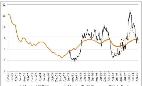
Figure 2: D-Star (Position of Curvature Peak in Years, 6-month CMA, Advanced 15 months and Inverted) and B-BBB Corporate Credit Spread, 1987-2016 (Monthly)

Comment: The position of the curvature peak (D-star) advanced by 15 months and inverted predicts future movements in the US corporate high yield spread between single B and BBB bonds. The negative correlation between the two series is minus 0.563 and D-star is strongly one-way Granger causal.

When D-star is included alongside measures of the three standard yield curve parameters, the regression results compare favourably with the principal components

16_{The Moody’s ‘Baa’ investment grade is equivalent to S&P’s ‘BBB’ rating.} 17

This index is constructed from the first principal component of the various national US financial stress indexes (FSIs), backfilled to 1987 using their major subcomponents, e.g. corporate credit spreads and the CBOE VIX

4 4.5 5 5.5 6 6.5 7 7.5 8 0 2 4 6 8 10 12 14 0 1/ 01 /1 98 7 0 1/ 03 /1 98 8 0 1/ 05 /1 98 9 0 1/ 07 /1 99 0 0 1/ 09 /1 99 1 0 1/ 11 /1 99 2 0 1/ 01 /1 99 4 0 1/ 03 /1 99 5 0 1/ 05 /1 99 6 0 1/ 07 /1 99 7 0 1/ 09 /1 99 8 0 1/ 11 /1 99 9 0 1/ 01 /2 00 1 0 1/ 03 /2 00 2 0 1/ 05 /2 00 3 0 1/ 07 /2 00 4 0 1/ 09 /2 00 5 0 1/ 11 /2 00 6 0 1/ 01 /2 00 8 0 1/ 03 /2 00 9 0 1/ 05 /2 01 0 0 1/ 07 /2 01 1 0 1/ 09 /2 01 2 0 1/ 11 /2 01 3 0 1/ 01 /2 01 5 0 1/ 03 /2 01 6 Yea rs P er Cent

(35)

decomposition. D-star contains additional information that, as I later show in Chapter 4, can help to predict a number of macro-finance variables besides those already mentioned, such as the ISM index of US business activity and popular measures of investors’ risk appetite. D-star falls ahead of major recessions and predates periods of financial turmoil. For example, according to estimates derived from generic Treasury yield data, D-star dropped significantly from a local peak of 7.45 years in December 2005 to 4.41 years in September 2007 ahead of the 2007/08 Financial Crisis and Great Recession. It has since rebounded to a current reading of around 7 years. These forewarnings do not occur because fixed income investors are any more prescient or better informed than others, but because it is easier to extract forward-looking information from the Treasury yield curve. These signals also may be purer because government bonds are less distorted by other factors, such as illiquidity and default risk. Long-dated government bonds constitute safe assets for several key investors types and, therefore, the demand for bond duration is, at the same time, often a demand for safe assets at that horizon. This, in turn, reflects a corresponding fall in investors’ overall risk appetite that will itself have future implications for the real economy.

This chapter is structured as follows: Section 3.2 reviews the recent preferred habitat and institutional finance literature. Section 3.3 examines the importance of duration management. In Section 3.5 I use the quadratic yield curve example to explain D-star, intuitively. Section 3.4 defines my measure of D-star. Section 3.6 describes the data and Section 3.7 provides monthly estimates for the position of the hump (D-star), using both security-level data from 1995-2016 and generic US Treasury spot yields over 1946-2016. Section 3.8 checks robustness. It compares the four parameter decomposition with principal components and estimates D-star directly from a Kalman filter technique. Section 3.9 concludes.

(36)

3.2 Review of the Preferred Habitat and Institutional Finance

Literature

Term premia are assumed to be negligible under the pure expectations hypothesis

(PEH), so rising interest rates rather than positive excess returns should follow periods of curve steepness (Fama and Bliss, 1987). Yet, it is well-documented (Ilmanen, 1995) that, in practice, three-month ahead excess returns (ex post) correlate with curve steepness (0.118). In addition, over the long-term when the mean-reverting behaviour of the yield curve washes out, the term structure still retains its concave shape. Thus, the return difference between a duration-matched bullet and barbell, i.e. the yield carry of a curve steepening strategy, earns an excess return, much like other examples of ‘carry’ in financial markets. Across four major bond markets – US, Germany, Japan and UK – the 1-5-10 year butterfly spread averaged +7bp (1986-2016) and +10bp (2000-16), showing that investors often pay premium prices for longer duration pay-offs. This contradicts the equality of horizon returns implicit in the PEH.

A mathematical analysis of these contributions (see Appendix A) shows how they can arise from: (1) the expectations of falling policy rates; (2) the excess demand for safe assets and (3) greater interest rate uncertainty. Each factor could be synonymous with sub-par future economic activity and a lower risk appetite among investors. These factors also affect the lateral position of the hump in the spot curve along the maturity axis. This position tells us the investment horizon where forward rates (and by implication expected policy rates) reach their maximum. This is explained (see Chapter 2 Appendix) because the duration-adjusted period change in spot yields is identically equal to the forward rate. When the hump occurs at shorter maturities, the economic outlook may be less favourable than normal and risk appetite low, while a hump positioned at an unusually long maturity could indicate risk-seeking behaviour and predate a future business cycle expansion. In cases where the PEH is superseded by the introduction of other factors into the pricing equation (e.g. the excess supply and demand for different maturities and/ or the option value of expected interest rate volatility), the position of the hump is also affected by the excess demand for safe assets and by the effects of greater interest rate uncertainty18. Ilmanen (1995) shows that, in

18

(37)

practice, excess supply and demand factors often dominate because the above butterfly

spread measure of yield carry only shows a modestly positive correlation with ex post

volatility (0.114).

The standard yield curve model is augmented to explain how these supply and demand factors influence US Treasury term premia. Tobin (1969) describes a portfolio balance

mechanism that adjusts the overall quantity of duration, liquidity and credit risk in response to shocks to the relative supplies of money (the zero duration asset) and other securities. Additional frictions are introduced by the preferred habitat hypothesis

(Modigliani and Sutch, 1966 and Vayanos and Vila, 2009) which opens up the possibility of market segmentation; through the importance of key investors in

institutional finance models with non-standard stochastic discount functions for asset

pricing (Adrian, Etula and Muir, 2010 and Haddad and Sraer, 2015) and with the existence of limits to arbitrage (Shleifer and Vishny, 1997). Modigliani and Sutch argue that bond interest rate risk should be measured relative to an investor's investment horizon, or preferred habitat, which vary by investor-type since different investors favour bonds of specific maturities. Investors’ desire to avoid risk: "...should lead them to hedge by staying in their maturity habitat, unless other maturities (longer or shorter) offer an expected premium sufficient to compensate for the risk and cost of moving out

of [their] habitat." (Modigliani and Sutch, 1966, p184). This means that yields are

determined by the local supply and demand conditions at each maturity. Adjacent securities in the maturity structure are assumed to be imperfect substitutes, with the inelasticity of yields directly related to the distance away from the preferred habitat, which helps to justify term premia. According to the preferred habitat view, the preference of investor clienteles for specific maturities becomes a significant determinant of bond yields, when the maturity structure of government debt supply change