Not Going to Take This Anymore: Multi-objective Overtime Planning for Software Engineering Projects

Not Going to Take This Anymore: Multi-objective

Overtime Planning for Software Engineering Projects

Filomena Ferrucci

, Mark Harman

, Jian Ren

and Federica Sarro

†_{University College London, CREST centre, London, WC1E 6BT, UK}

Abstract—Software Engineering and development is well-known to suffer from unplanned overtime, which causes stress and illness in engineers and can lead to poor quality software with higher defects. In this paper, we introduce a multi-objective decision support approach to help balance project risks and duration against overtime, so that software engineers can better plan overtime. We evaluate our approach on 6 real world software projects, drawn from 3 organisations using 3 standard evaluation measures and 3 different approaches to risk assessment. Our results show that our approach was significantly better (p <0.05) than standard multi-objective search in 76% of experiments (with high Cohen effect size in 85% of these) and was significantly better than currently used overtime planning strategies in 100% of experiments (with high effect size in all). We also show how our approach provides actionable overtime planning results and inves-tigate the impact of the three different forms of risk assessment.

I. INTRODUCTION

Poor overtime planning is particularly pernicious in the software industry. Facing a combination of estimate inaccuracy and time-to-market pressure, software engineers are often coerced into high levels of unplanned overtime, leading to dissatisfaction, depression, and defects. Inability to plan and budget for overtime leads to hastily arranged, unplanned overtime and the familiar spectre of the ‘death march project’ [1].

This has a detrimental effect on the quality of the lives of the software engineers unfortunate enough to be involved and also of the quality of the software that they produce. As might be expected, the problems of unplanned overtime have been widely reported upon in the occupational health literature, which contains many systematic studies of its unfortunate side effects on profes-sionals and the products and services they provide [2], [3], [4]. There is also evidence for the harmful effects of unplanned overtime specifically on software engineering professionals and the software they produce, though it is perhaps surprising how little this phenomenon has been systematically studied, given the widespread belief that it is so prevalent [1], [5]. A controlled study of 377 software engineers found positive correlations (p <0.05) between unplanned overtime and several widely-used stress and depression indicators [6]. There is also evidence that the deployment of overtime can lead to increased software defect counts [7].

Fortunately, there is also case study evidence that proper planning leads, not only to greater software engineer job satisfaction, but also to improved customer satisfaction in the resulting software products [8]. Looking to the wider (non-software-engineering specific) literature, we can also find evidence that planned overtime has few, if any, of the harmful side-effects that so-often accompany unplanned overtime [9]. This evidence all points to the need for research into decision support for software engineers to help them better plan for overtime, balancing the need for overtime against project overrun risks and budgetary constraints.

The software engineering literature contains many excellent examples of research on software engineering support techniques for a wide range of engineering tasks such as testing, design and maintenance. This work has contributed to the software-enabled development environments that many software engineers now take for granted [10]. However, sadly, there has been no research aimed at providing support to software engineers in their attempts to plan for overtime.

This paper addresses this problem. We introduce an approach to support software engineers in better planning for overtime, while managing risk. The problem is to find the right balance between the conflicting objectives of reducing project duration, overtime, and risk.

Complex multi-objective decision problems with competing and conflicting constraints such as this are well suited to Search Based Software Engineering (SBSE) [11], which has proved able to provide decision support for other early-stage development activities, notably requirements engineering [12], [13], [14]. We believe that this is the first time that an approach has been introduced to provide decision support for software engineers attempting to reconcile these complex and difficult problems. More specifically, the primary contributions of the paper are as follows:

1) We introduce a multi-objective search based formulation of the project overtime planning problem. Our approach is able to balance trade offs between project duration, overrun risk, and overtime resources for three different risk assessment models. It is applicable to standard software project plans, such as those constructed using the Critical Path Method, widely adopted by software engineers and implemented in many tools.

2) We present an empirical study on 6 real world software projects, ranging in size from a few person weeks to roughly four person years. This leads to 54 different experiments, comparing our proposed algorithm (with domain specific crossover operator) to the standard multi-objective algorithm and random search. The results reveal that our approach was significantly better than standard multi-objective search in 76% of experiments and was significantly better than random search in 100% experi-ments. The standard multi-objective approach significantly outperforms our approach in none of the experiments. We repeated the experiments to compare our approach with standard overtime planning strategies reported in the liter-ature. This revealed that our approach always significantly outperforms these standard strategies with high effect size. 3) We present case studies using Pareto fronts obtained by our approach to illustrate how they yield actionable insights into project planning tradeoffs. We also use our approach to investigate the different risk assessment models that might be adopted.

The rest of the paper is organised as follows: In Section II the overtime planning problem is defined. Section III introduces our search based approach to solving this problem using a multi-objective Pareto optimal approach. Section IV describes the method used in our empirical studies, the results of which are presented in Section V. Section VI analyses the limitations of the present study, while Section VII describes the context of related work in which the current paper is located. Section VIII concludes and presents directions for future work.

II. PROBLEM FORMULATION

Our formulation of the problem starts from the Work Breakdown Schedule (WBS) produced by the software engineer, which we formalise here for clarity. Such a WBS can be produced by many project planning tools, such as Microsoft project (the tool used by all the organisations that provided the real world schedules used to evaluate our approach in this paper).

Let a project schedule be represented as an

acyclic directed graph consisting of a node set

W P = {wp1, wp2, ..., wpn} of work packages and an

edge set DEP ={(wpi, wpj) :i=6 j,1≤i≤n,1≤j ≤n}

of dependencies between elements of WP, where wpj can start

only when wpi has completed. WP and DEPS form a graph,

the set of paths, Π, of which, denote the dependence-respecting orderings of work packages to be undertaken to complete the project. Associated with each work package,wpi, is the estimated effort, ei, required to complete wpi and also its estimated duration Duration(wpi). Based on this, the duration of each

pathp∈Π through the project dependence graph is given by

Durationp=

X

∀wp∈p

Duration(wp) (1) and the total estimated shortest possible duration of the project is given by any maximal length (or ‘critical’) path inΠ. This is a for-malisation of the well-known ‘Critical Path Method’ [15], which has been widely used in project planning for several decades. Though there may be several equal length critical paths (for which no other path is longer) it is traditional to select one and to refer to it asthe critical path,CP, a convention we adopt hereinafter.

Our problem is to analyse the effects of choices of overtime assignments, each of which seeks to minimize project duration, risk of overrun and the amount of overtime deployed. This can be formulated as a three objective decision problem in which the three objectives of duration, risk and overtime are conflicting minimisation objectives.

We represent a candidate solution to our problem as an assignment of overtime to work packages. A feasible solution is an assignment of a certain number of extra hours to each work package, denoted by Overtime(wpi)subject to the following constraint: 0 ≤ Overtime(wpi) ≤ M axOvertime(wpi),

where M axOvertime(wpi) is the maximum assignable

overtime to the ith work package and depends on the effort

ei and the maximum overtime assignable per day1_.

We shall use computational search to seek an allocation of overtime for all work packages that minimises each of the three objectives of Overtime (O), Project Duration (D) and Risk of Overrun (R). We therefore measure fitness as a triple hO, D, Ri, whose components are defined as follows:

1_{The length of a working day and maximum allowed overtime are country}

specific parameters to our approach, determined by legal and governance procedures in place. In this paper we set these to 8 hours for a working day and 3 hours per day maximum overtime.

Overtime(O) is the amount of time worked on each work package beyond the individual time limit per day summed over all work packages. More formally:

O= n

X

i=0

Overtime(wpi) (2)

Project Duration(D) is the estimated duration (i.e., the length of the critical path). More formally:

D= X wp∈CP

Duration(wp) (3) We define the risk of overrun in terms of the risk of overrun associated to each path,p, in the project schedule:

riskp= Durationp DurationCP

(4) The closer riskp is to 1.0, the greater the chance that an overrun on a work package along pathpwill causepto supersede the current critical path as the determinant of project duration (pthus becoming the new critical path due to the overrun).

We use three different approaches to the measurement of Risk of Overrun (R), each of which combines the path risk

riskp, above into an overall project risk, R, as follows: R=RAvgRisk=

P

p∈Πriskp

|Π| (5)

R=RM axRisk=maxp∈Π−CPriskp (6) R=RT rsRisk(L) =| {p·p∈Π∧riskp> L} |

|Π| ·100 (7)

These are, respectively, average, maximal, and threshold level risks. Average risk is suited to the engineer who is ‘risk averse’; it assumes that any overrun on any path could be a problem. This is ‘risk averse’ in the sense that it reflects a pessimistic belief that ‘anything that can go wrong will go wrong’. Maximum risk is better suited to the engineer who is more concerned that the critical path is not disrupted, but who is relaxed about overruns in non-critical paths that do not threaten to supersede the critical path, as these could be absorbed into the project schedule. Threshold risk allow the engineer to choose a risk level, making risk level a parameter to the overall approach (which we set to 0.75 in this paper).

Of course, overtime allocation is a disruptive process; it can change the critical path. This is one of the motivations for decision support: engineers cannot be expected to understand the impact of proposed overtime allocations on the critical path, while simultaneously balancing budgets, durations, and estimates of overruns. These are precisely those problems for which we need the kind of automated analysis we introduce in this paper.

III. THESOLUTIONAPPROACH

Our solution uses Search Based Software Engineering (SBSE) [16], [11], for which it is established best practice to define a rep-resentation, fitness function and computational search algorithm [17]. Since our formulation is a triple objective formulation we also need to decide how to handle multiple objectives.

Handling Multiple Objectives: In our case, the three

objectives are measured on orthogonal scales so we use Pareto optimality, which states: “A solution x1 is said to dominate

another solutionx2, ifx1is no worse thanx2 in all objectives

Pareto optimality means that we do not suggest to the engineer a single proposed solution. That would not be realistic. No engineer would trust an automated tool to provide a single overtime allocation. Rather, we seek to provide a decision support tool, by showing the solutions in a space of trade offs between the three objectives, allowing the engineer to see the trade offs between them.

Using Pareto optimality we can plot the set of solutions found to be non-dominating (and therefore equally viable). In the case where there are three objectives, such as ours, this leads to a three dimensional Pareto surface, though we can also project this surface onto a two dimensional Pareto front to focus any two objectives of interest. The shapes of such surfaces and fronts can yield actionable insights. For example, where there is a knee point (a dramatic switch in the material values of trade off between objectives), this guides decision making (See Section V).

Representation: Feasible solutions to the problem defined in Section II are assignments of a certain number of overtime hours to each work package. We encoded them as chromosomes of length n, where each gene represents the number of extra hours assigned to each work package. The initial population, composed by n chromosomes, was randomly obtained by assigning to each wpi an overtime ranging from 0 to M axOvertime(wpi).

Fitness: To evaluate the fitness of each chromosome we

employed a multi-objective function to simultaneously minimise the objectives described in Section II, namely Project Duration, Overtime, and Risk of Overrun. We report results for each overrun risk assessment measure (AvgRisk, MaxRisk, and TrsRisk) sepa-rately to explore the effects of each approach to risk assessment.

Computational Search: As a ranking method, we employed a

widely used Multi-Objective Evolutionary Algorithm (MOEA), namely NSGAII [18]. However, it is insufficient merely to apply a generic algorithm like NSGAII ‘out of the box’; we need to define problem-specific genetic operators to ensure best performance. In the case of genetic algorithms such as NSGAII the crossover operator plays a pivotal role [19], [20], [21] and thus forms a natural focus for such problem-specific algorithm design.

We therefore introduce a variant of NSGAII (which we call NSGAIIv) specifically for the overtime planning problem.

NSGAIIvexhibits the same selection and crowding distance

char-acteristics as the standard NSGAII but exploits a new crossover operator. Our crossover operator aims to preserve genes shared by the fittest overtime assignments, thereby avoiding the well-known disruptive effects of crossover [19]. It is defined as follows:

LetP1andP2be parent chromosomes,Cthe point of cut

ran-domly selected in the parents, andO1 andO2the new offspring.

For the genes placed beforeC,O1 andO2inherit the genes of

P1 andP2, respectively. While for each genegi placed after C,

O1(gi) = n_max(P 1(gi),P2(gi)),p=0.5 min(P1(gi),P2(gi)),p=0.5 o O2(gi) = (P1(gi) +P2(gi))/2

Note that when the parent genes hold the same characteristic (i.e., same quantity of overtime) they are retained in both offspring, otherwise we generate two different genes for the offspring: one that inherits the gene from mother or father with equal probability and one that inherits both parent characteristics in terms of overtime average.

IV. THEDESIGN OF THEEMPIRICALSTUDY This section explains the design of our empirical study; the research questions we set out to answer and the methods and statistical tests we used to answer these questions.

A. Research Questions

We seek to answer five research questions, each of which builds on its predecessor to develop the evidence for the validity, performance, usefulness, and insights gained from our approach to overtime planning.

RQ1 (SBSE Validation): How do NSGAII and NSGAIIv

perform compared to random search? In any attempt at an SBSE formulation of a problem this is a standard ‘baseline’ question asked. If a proposed formulation does not allow an intelligent computational search technique to outperform random search convincingly, then there is clearly something wrong with the formulation. This question is thus adopted in SBSE research as a preliminary ‘sanity check’ [22].

RQ2.1 (Comparison to State of the Art Search): How does

NSGAIIvperform compared to NSGAII? Outperforming random

search is necessary, but not sufficient. In order for a proposed approach to be adopted it must also outperform the state of the art for the problem in hand. In this case, there is no prior work on the problem of planning overtime on software projects. We therefore compare our approach, N SGAIIv, to the standard version of the algorithm (NSGAII), applied to our formulation.

RQ2.2 (Usefulness): How does NSGAIIv perform compared

to currently used overtime planning approaches? While outperforming a standard multi-objective search may be a valuable technical result, in order to be useful to software engineers, our approach must also outperform existing overtime management strategies used by practicing software engineers. We therefore repeat the experiments in RQ2.1, but for RQ2.2 we compare our approach with three currently used strategies.

RQ3 (Insight): Can our approach yield useful insights into the trade offs between objectives for real world software projects? To provide decision support it is insufficient to demonstrate that our approach outperforms engineers’ current practices. We must also provide evidence that our approach yields insights into the nature of the overtime planning problem. In order to do this, we need to give examples of actionable insights obtainable from the application of our approach to the real world software projects of the empirical study.

RQ4 (Impact of Risk Assessment Models): What is the

difference between the three approaches to risk measurement? If our approach is demonstrated to outperform state of the art and current practice and it also provides useful insights, then we can use it to explore the three different risk assessment models we implemented (average, maximal, and threshold risk assessment). Since these different assessments of risk reflect different priorities in software engineers’ management of risk, the findings shed light on the impact of different approaches to risk management in overtime planning.

B. Software Projects Used in the Empirical Study

Table I summarises the key information concerning the 6 projects used in the empirical study. The projects came from three different organisations, involved different kinds of software engineering development and had different sizes, ranging from 60 to 245 work packages and from a few person weeks to several person years in duration.

DB2 concerned the next release of a large data-intensive, multi-platform software system, written in several languages including DB II, SQL, and .NET. Webdelivered a web-based IT sales system across North America. The project included the development and testing of website, search engine and order management and tracking.

TABLE I

SOFTWARE PROJECTS USED IN THE EMPIRICAL STUDY. EFFORT IS MEASURED IN NORMALISED PERSON HOURS.

Project #WPs #Dependencies Effort Brief Description.

DB2 120 102 594 A multi-platform database upgrade involving several languages such as DB2, SQL and .NET

Web 245 247 6,664 A web-based purchase order system development

Quote 60 64 547 An enhancement of an existing system to include on-demand conversion of quotes to orders

Oracle 106 105 5,390 A large-scale Oracle database migration with tight data security constraints

Price 72 71 1,570 A client-side sales system upgrade to offer additional features to users

CutOver 95 68 2,356 Details cannot be revealed because of a Non Disclosure Agreement with the project data provider

Quotewas a system developed for a large Canadian sales

company to provide on-demand conversion of quotes to orders.

Oracle was large scale database upgrade, migrating an old,

yet mission-critical, Oracle system. The information that was migrated had an estimated value to the organisation of several million dollars and formed the cornerstone of the organisation’s operations. Pricewas an enhancement to the client side of a sales system to provide improved pricing and features for discounts, vouchers, and price conversions. The details of project

CutOverare the subject of a Non-Disclosure agreement and

so cannot be published.

C. Multi-Objective Evaluation Measurements Used

Assessing the performance of a computational search algorithm for a single objective optimisation problem typically requires observations about the best solution found. This approach is not applicable for multi-objective optimisation problems because there are a set of candidate solutions, each of which is said to be ‘non-dominating’. That is, each is incomparable to the others because no other solution has better values for all objectives. Analysis of graphical plots of the solutions can provide some indications of performance, but it provides a qualitative evaluation and cannot provide a quantitative assessment of the quality of solutions from one approach relative to another. A robust evaluation requires that qualitative evaluations be augmented by a more quantitive evaluation.

To provide this quantitative assessment we employ three solution set quality indicators, namely Contributions (IC), Hypervolume (IHV), and Generational Distance (IGD). To compute these we normalise fitness values to avoid unwanted scaling effects [23] and compute a reference front of solutions,

RS, which is the set of non-dominated solutions found by the union of all approaches compared [24].

The IC quality indicator is the simplest measure. It measures

the proportion of solutions given by an algorithm, A, that lie on the reference front RS[25]. The higher this proportion, the moreAcontributes to the best solutions found by the approaches compared, and so the better is the quality of its solutions. IC is a simple and intuitive measure, but it is affected by the number of solutions produced, unfavourably penalising algorithms that might produce ‘few but excellent’ solutions. This is why we also consider two other measures of solution quality, IHV andIGD.

The IHV quality indicator [26] calculates the volume (in the objective space) covered by members of a non-dominated set of solutions from an algorithm of interest. The larger this volume, the better the algorithm, because the more it captures of the non-dominated solution space. Zitzler demonstrates [27] that this hypervolume measure is also strictly ‘Pareto compliant’. That is, the hypervolume ofA is higher thanB if the Pareto set of Adominates that ofB. By using a volume rather than a count, this measure is also less susceptible to bias when the numbers of points on the two compared fronts are very different.

TheIGD quality indicator [28] computes the average distance between the set of solutions,S, from the algorithm measured and the reference setRS. The distance between S andRS in annobjective space is computed as the averagen-dimensional Euclidean distance between each point in S and its nearest neighbouring point in RS. We can think of IGD as the distance between the front S and the reference front RS in then-dimensional objective space of the problem.

D. Inferential Statistical Test Methods Used

Due to the stochastic nature of evolutionary algorithms, best practice requires the use of careful deployment of inferential statistical testing to assess the differences in the performance of the algorithms used [17], [29]. We therefore performed 30 independent runs per algorithm, per risk assessment measure, per project to allow for such statistical testing.

To analyse the normality of distributions we employed the Shapiro test [30]. As we expected, many of our samples showed no evidence that they come from normally distributed populations, making thet-test unsuitable. We therefore used the Wilcoxon test [31] to check for statistical significance. Using the Wilcoxon test is a safe test to apply (even for normally distributed data), since it raises the bar for significance, by making no assumptions about underlying data distributions. We set the confidence limit,α, at 0.05 and applied the standard Bonferroni correction (α/K, where K is the number of hypothesis) in cases where multiple hypotheses were tested.

As has been previously noted in advice on statistical testing of algorithms such as these [29], it is inadequate to merely show statistical significance alone; we also need to know whether the effect size is worthy of interest. Therefore, in order to additionally assess the effect size, we used Cohen’s d, the results of which are usually considered small for0.2≤d <0.5, medium for0.5≤d <0.8, and large ford≥0.8 [31].

To answer RQ1 we implemented a random search to be compared with NSGAII and NSGAIIv. The random search

assigns randomly to each work package of the project, an overtime varying from 0 to the maximum overtime assignable. The resulting Pareto fronts were compared for statistically significant differences with those produced by NSGAII and NSGAIIv, using the quality indicators explained in Section IV-C.

In this sanity check we used the Wilcoxon test and for significance also performed a Cohen effect size test in all results. We do not wish to devote too much space to RQ1, since it is only a ‘sanity check’, preferring to devote more space to the answers to RQs 2–4, which concern more scientifically important evidence for the performance and usefulness of our approach. To answer RQ2.1 we compared NSGAII and NSGAIIv in terms of

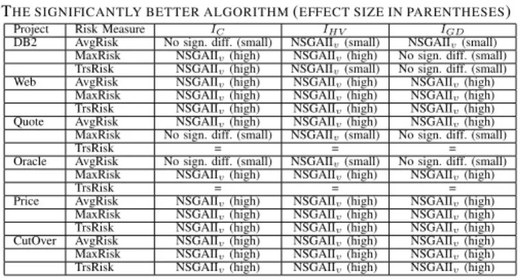
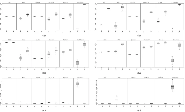
the quality indicators for statistical significance and effect size, as for RQ1, but additionally presenting the results using boxplots to give a pictorial account of the distributions of results obtained.

TABLE II

CONFIGURATIONS EXPLORED TO TUNE THE TWO ALGORITHMS

Configuration Pop. Size Generations Fitness Evals Very Small (VS) 50 5,000 250,000 Small (S) 100 2,500 250,000 Medium (M) 200 1,250 250,000 Large (L) 500 500 250,000 Very Large (VL) 1,000 250 250,000 TABLE III

BEST OBTAINED CONFIGURATIONS FORNSGAIIANDNSGAIIv

Project _NSGAIIMaxRisk_{NSGAIIv NSGAII}AvgRisk_{NSGAIIv NSGAII}TrsRisk_NSGAIIv

DB2 M VL VL VL L VL Web S S VL VL M M Quote VL VL VL VL VL VL Oracle VL VL VL VL S S Price L VL VL VL M M CutOver S VS VS VL VL S

To answer RQ2.2 we compared NSGAIIvto standard overtime

management strategies. That is, we implemented three strategies currently used, and compared the results to our NSGAIIv

approach using the same tests as we performed to answer RQ2.1. To answer RQ3 we analysed the Pareto fronts produced by our approach in order to identify useful trade offs among different goals and to discover knee points by means of graphical plots. We answer RQ4 by exploring the differences between the three risk assessment approaches studied in the paper (in terms of the Pareto surfaces that capture the solution space for each form of assessment).

E. Parameter Tuning and Setting

An often overlooked aspect of research on computational search algorithms lies in the selection and tuning of the algorithmic parameters, which is necessary in order to ensure fair comparison, but which often goes unreported and, thereby, hinders any potential replication. In order to facilitate replication of our findings, we report the method adopted for algorithmic parameter tuning and selection in this section.

We evaluated, for each algorithm, five different configurations characterised by very small, small, medium, large, and very large values for population as detailed in Table II. All configurations were allowed an identical budget of fitness evaluations (250,000), thereby ensuring that all require the same computational effort, though they may differ in parameter settings. We executed NS-GAII (NSNS-GAIIv) with each configuration 30 times and collected

the corresponding IC,IHV, andIGD values, testing for signifi-cant differences using the Wilcoxon Test. Table III reports the best configurations we selected for each algorithm and risk measure. The rest of our parameter settings for both algorithms were typical standard settings. We report them here for completeness and replicability. For population sizen, at each generation,n/2

applications of the single point crossover operator are used to construct offspring. The crossover operator performs crossover with a probability 0.5. The same number of mutations were performed, where the value of each gene is modified with a probability of 0.3. The mutation operator randomly assigns a new value between 0 andM axOvertime(wp). We employed binary tournament selection based on dominance and crowding distance, and in tied tournaments one of the two competitor parents is chosen at random (with equal probability for both).

V. ANALYSIS OFRESULTS

This section presents the results obtained from our experiments for RQs 1–4 set out in Section IV-A.

TABLE IV

THE SIGNIFICANTLY BETTER ALGORITHM(EFFECT SIZE IN PARENTHESES)

Project Risk Measure IC IHV IGD

DB2 AvgRisk No sign. diff. (small) NSGAIIv(small) NSGAIIv(small)

MaxRisk NSGAIIv(high) NSGAIIv(high) No sign. diff. (small)

TrsRisk NSGAIIv(high) NSGAIIv(small) No sign. diff. (small)

Web AvgRisk NSGAIIv(high) NSGAIIv(high) NSGAIIv(high)

MaxRisk NSGAIIv(high) NSGAIIv(high) NSGAIIv(high)

TrsRisk NSGAIIv(high) NSGAIIv(high) NSGAIIv(high)

Quote AvgRisk NSGAIIv(high) NSGAIIv(high) NSGAIIv(high)

MaxRisk No sign. diff. (small) NSGAIIv(small) No sign. diff. (small)

TrsRisk = = =

Oracle AvgRisk No sign. diff. (small) NSGAIIv(small) No sign. diff. (small)

MaxRisk NSGAIIv(high) NSGAIIv(high) NSGAIIv(high)

TrsRisk = = =

Price AvgRisk NSGAIIv(high) NSGAIIv(high) NSGAIIv(high)

MaxRisk NSGAIIv(high) NSGAIIv(high) NSGAIIv(high)

TrsRisk NSGAIIv(high) NSGAIIv(high) NSGAIIv(high)

CutOver AvgRisk NSGAIIv(high) NSGAIIv(high) NSGAIIv(high)

MaxRisk NSGAIIv(high) NSGAIIv(high) NSGAIIv(high)

TrsRisk NSGAIIv(high) NSGAIIv(high) NSGAIIv(high)

Results for RQ1 (SBSE Validation): We observed that both

NSGAII and NSGAIIv achieved superior values compared to

random search for all three quality indicators (i.e., IC, IHV,

IGD) and on all six projects. The Wilcoxon test results showed that for all 54 experiments (3 indicators, 3 risk assessment approaches, and 6 projects) the quality indicators achieved by NSGAII and NSGAIIv were significantly better than those

of random search with a Cohen effect size ‘high’. Thus, we conclude that there is strong empirical evidence that our formulation passes the sanity check denoted by RQ1.

Results for RQ2.1 (Comparison to State of the Art Search): Table IV presents the results of the significance tests and effect size test. We observe that our algorithm, NSGAIIv,

outperforms the standard NSGAII in 41 out of 54 (76%) experiments and in 35 of these 41 (85%) it does so with a Cohen effect size ‘high’, whilst the standard approach does not outperform our approach in any of the experiments.

In more detail, we observe that NSGAIIvachieved significantly

superiorIC values with respect to NSGAII in 13 out 18 cases with a high effect size. Only in two cases (i.e., projects Quote

andOraclewith TrsRisk) the two distributions were identical,

while in three cases (i.e., projects DB2,Quote, andOracle

with AvgRisk, MaxRisk, and AvgRisk, respectively) no signifi-cant differences were found. ForIHV, we observe that NSGAIIv

significantly outperformed NSGAII in 16 out of 18 cases with a high and small effect size (12 and 4 respectively), while in the remaining two cases (i.e., projectsQuoteandPricewith TrsRisk) the two distributions were identical. For the third quality evaluation measurement, IGD, NSGAIIv achieved significantly

better values than NSGAII in 11 out of 18 cases with a high effect size and in one further case there was a significant difference (but small effect size). In 4 cases there were no significant differences between the two approaches and, again, on projectsQuoteand

Oraclewith TrsRisk the two distributions were identical.

We can also get a more qualitative sense of the distributions of results for the two approaches from the box plots shown in Figures 1, 2 and 3. From these box plots we can see that the vari-ance in the results from both algorithms is lower for the threshold risk assessment measure than the other two. Subsequent results for RQ3 and 4 (see below) suggest that this is because there are simply fewer solutions available when threshold risk is used, due to the constraints the threshold imposes. For the other two risk assessment measures, variance is project specific, but low in all cases irrespective of the project concerned: standard deviation values ranged between 0.01 to 0.06 overall projects exceptDB2

(a)

(b)

(c)

Fig. 1. Boxplots for the average risk assessment approach (AvgRisk), evaluated using the quality measuresIC(a),IHV(b), andIGD(c) applied to NSGAII (Algorithm A) and NSGAIIv(Algorithm B)

Results for RQ2.2 (Usefulness): In order to answer RQ2.2, we need to define ‘current overtime planning practice’. There is evidence that current overtime practice employs what we term ‘margarine management’; spreading the overtime thinly and evenly over all work packages [32]. We can therefore compare our approach to this documented Overtime Management Strategy (OMS). There are two other natural strategies (often referred to anecdotally in the literature): loading overtime onto the critical path to reduce completion time and loading it onto the later half of the project to compensate for earlier delays.

Table V reports the mean values of each of the three quality assessment indicators obtained for 30 runs of all projects using NSGAIIv and the three OMS practices defined above.

The Wilcoxon Test confirmed that all the indicators obtained employing NSGAIIv were significantly better than those

obtained with each and all of the OMS practices and with a high Cohen effect size in every case.

As an example, Figure 4 shows the reference fronts obtained by NSGAIIv and the three OMS practices for the largest project

Web. In this and all subsequent figures, overtime is measured in total overtime hours committed to the project, while project duration is measured as the length of the critical path (in days). While Table V gives the precise technical answer to RQ2.2, Figure 4 provides a more qualitative assessment of the meaning of this technical finding. As can be seen, the Pareto surface produced by NSGAIIv offers many more points (sometimes

revealing quite clearly the shape of the solution space). By contrast, the currently used approaches appear to merely

(a)

(b)

(c)

Fig. 2. Boxplots for the maximal risk assessment approach (MaxRisk), evaluated using the quality measuresIC(a),IHV(b), andIGD(c) applied to NSGAII (Algorithm A) and NSGAIIv(Algorithm B)

TABLE V

MEAN VALUES OF THE QUALITY INDICATORS FORNSGAIIvAND THE THREE

CURRENTOVERTIMEMANAGEMENTSTRATEGIES(OMS).

Project Risk Measure IC IHV IGD

NSGAIIv OMS NSGAIIv OMS NSGAIIv OMS

DB2 AvgRisk 0.998 0.002 0.614 0.259 0.001 0.070 MaxRisk 0.998 0.002 0.440 0.116 0.000 0.237 TrsRisk 0.999 0.001 0.461 0.000 0.000 0.456 Web AvgRisk 0.993 0.007 0.544 0.226 0.000 0.016 MaxRisk 0.962 0.038 0.559 0.257 0.008 0.195 TrsRisk 0.961 0.039 0.551 0.203 0.001 0.060 Quote AvgRisk 0.997 0.003 0.475 0.269 0.000 0.013 MaxRisk 0.997 0.003 0.376 0.148 0.000 0.128 TrsRisk 0.998 0.002 0.424 0.116 0.000 0.161 Oracle AvgRisk 0.994 0.006 0.611 0.329 0.000 0.013 MaxRisk 0.994 0.006 0.630 0.256 0.000 0.033 TrsRisk 0.916 0.084 0.645 0.371 0.007 0.038 Price AvgRisk 0.994 0.006 0.583 0.247 0.000 0.024 MaxRisk 0.992 0.008 0.696 0.428 0.000 0.032 TrsRisk 0.987 0.013 0.346 0.004 0.001 0.116 CutOver AvgRisk 0.996 0.004 0.609 0.305 0.000 0.028 MaxRisk 0.910 0.090 0.544 0.260 0.015 1.285 TrsRisk 0.970 0.030 0.700 0.277 0.002 0.235

pick relatively arbitrary solutions, which are sub-optimal (far away from the frontier) and which thus denote little more than rather inaccurate guesses.

Results for RQ3 (Insight): To answer RQ3 we present

examples of the Pareto fronts obtained using NSGAIIv,

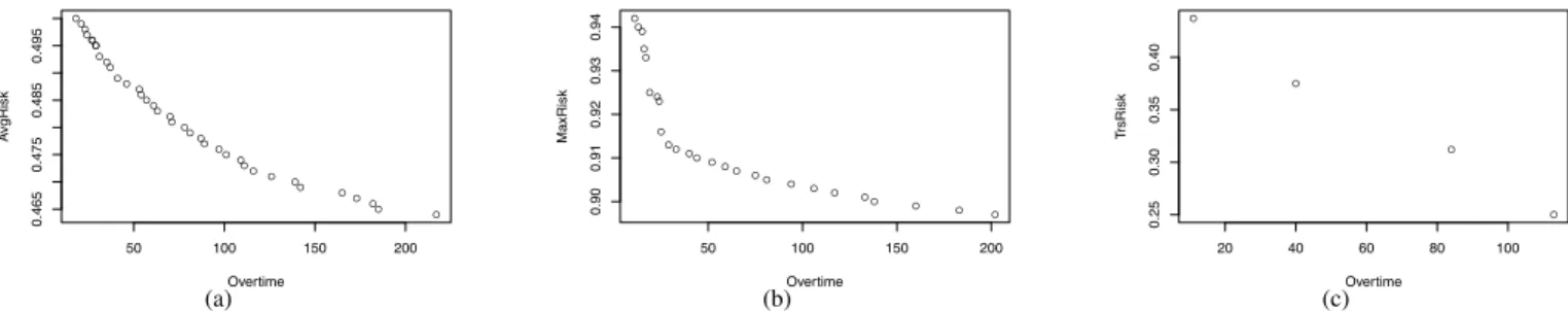
illustrating how they reveal insights into the trade off between risk, duration, and overtime. Software engineers can exploit this information when making decisions about software project overtime planning. For example, Figure 5 reports the two-dimensional projections of the Pareto front obtained by executing NSGAIIv on the Price project, projecting the

result onto the two objectives of overtime and risk. Such a 2D projection depicts the tradeoff between the spend on the overtime

(a) (b) (c)

Fig. 4. Pareto surfaces for NSGAIIv(depicted by the circles) and for all of the three Overtime Management Strategies (depicted by the triangles) obtained using each of the three risk assessment approaches: AvgRisk(a), MaxRisk(b), and TrsRisk(c) for the projectWeb.

(a)

(b)

(c)

Fig. 3. Boxplots for the threshold risk assessment approach (TrsRisk), evaluated using the quality measuresIC(a),IHV(b), andIGD(c) applied to NSGAII (Algorithm A) and NSGAIIv(Algorithm B)

budget and the impact this has on reducing risk according to the three risk assessment measures. Several insights are immediately obvious from these three plots. We can see that using a threshold risk level reduces the scope for choice in selection of an overtime budget (fewer points on the Pareto front in Figure 5(c)). Such a threshold should thus only be considered by an engineer who is certain they have selected an appropriate risk level.

By contrast, the risk averse engineer who seeks to reduce average risk overall, is presented with a relatively smooth trade off between the cost of overtime and the risk reduction it affords (Figure 5(a)).

For the engineer who seeks to reduce only the maximal risk

there is clear guidance from the shape of the Pareto front for Figure 5(b): A knee point in the front occurs at a budget of around 25 hours overtime. Up to this knee point along the horizontal axis, modest increases in overtime spend will yield sharp correspond-ing reductions in maximal risk. However, increascorrespond-ing overtime spend above this knee point of 25 hours, the engineer has to commit significantly more overtime spend to further reduce risk. This finding has actionable conclusions for the software engineer planning overtime on this project. Without the benefit of the insights provided by our overtime planning analysis, it would naturally be tempting to seek the maximum overtime budget allowable (202 hours) to ensure that there is the largest resource available to deal with problems. However, this inherently conservative approach will likely lead to stress, illness and defects as widely reported in the literature [1], [2], [3], [4], [6], [7], [8]. Fortunately, with the benefit of our overtime planning analysis, it is revealed that there is a much more compelling alternative. With a budget of only 25 hours overtime (only about 12% of the maximum allowable) it is possible to achieve more than 50% of the risk reduction achievable by the conservative approach which maximises overtime to minimise overrun risk. Of course, it will be for the software engineer to make the final decision concerning overtime planning. However, using our analysis, he or she can clearly see that a budget of around 12% of the maximum overtime allowable would be ideal in principle and this is an important input to the final decision, bearing in mind the well-known problems associated with overuse of overtime. Using these Pareto fronts the software engineer can thus obtain answers to questions like ‘how much spend on overtime is cost effective for my project plan?’ and ‘what must I spend to reduce average risk byx%?’. Such answers provide decision support to the engineer faced with the task of negotiating an overtime budget with their manager. They may also support decisions about how to most effectively deploy a budget to reduce risk. Space does not permit us to show results for all 6 projects. However, similar examples of interesting insights were observed for other projects.

Results for RQ4 (Impact of Risk Assessment Models): To

answer RQ4 we use the 3D visualisations of the Pareto surface, thereby showing the trade offs between all three objectives of overtime, duration, and risk. This allows us to compare the influence of the three different risk assessment measurements. Once again, space does not allow us to present all 18 plots, so we present (in Figure 6) the results from one project (Price) that is typical of the overall trends we observed in all projects. The most immediately obvious effect is the number of

● ● ● ● ● ● ● ● ● ● ● ● ● ● ● ● ● ● ● ● ● ● ● ● ● ● ● ● ● ● ● ● ● ● ● ● ● 50 100 150 200 0.465 0.475 0.485 0.495 Overtime A vgRisk (a) ● ● ● ● ● ● ● ● ● ● ● ● ● ● ● ● ● ● ● ● ● ● ● ● ● ● 50 100 150 200 0.90 0.91 0.92 0.93 0.94 Overtime MaxRisk (b) ● ● ● ● 20 40 60 80 100 0.25 0.30 0.35 0.40 Overtime TrsRisk (c)

Fig. 5. 2D Pareto surface projections for each of the three risk assessment approaches: AvgRisk(a), MaxRisk(b) and TrsRisk(c) for the projectPrice.

solutions offered by each approach to risk assessment. This can be clearly observed from the density of the Pareto surfaces shown in Figure 6 and it reveals an inherent property of these three risk assessment methods: the AvgRisk surface has 2,452 solutions, while MaxRisk has 1,228 and TrsRisk has only 182. Over all six projects the median number of solutions found was 2,535 for AvgRisk, 1,473 for MaxRisk and 190 for TsrRisk indicating that Figure 6 is not atypical.

The risk averse planner seeks to reduce average risk over all project paths and so this leads to many different trade offs and the largest number of potential solutions. The software engineer who has confidence in the applicability of the Critical Path Method (and thus seeks to reduce risks along this path) has fewer solutions available. However, this ‘CPM-confident’ engineer still has many solutions from which to choose and, more importantly, a continuous set of increasing degrees of trade off along each of the three dimensions of choice. By contrast, the engineer who is so confident in their risk assessment that they set a threshold risk level will have few solutions from which to choose; the threshold choice constrains the solutions. In particular, it reduces the number of projected project durations from which the engineer can choose.

The Pareto surfaces in Figure 6 also reveal an effect we found in four of the projects (Web, Oracle, Price and

CutOver): the risk averse (AvgRisk) form of assessment leads

to less pronounced changes in the dynamics of the trade off compared to the other two approaches. This can clearly be seen from the shape of Figure 6(a) compared (for example) to Figure 6(b); the former depicts a more gentle gradient through any arbitrary projection of the surface compared to the latter. This finding reflects the fact that the risk averse engineer seeks to minimise all risks, thereby reducing difference between choices, whereas the engineer who focuses effort on the critical path has a more pronounced impact of the choices they make on the solutions offered. Of course, there is no ‘free lunch’: we can also see that the risk averse engineer typically has to commit greater resources to satisfy their strategy than the others (solutions appear further to the right, denoting high overtime costs, in Figure 6(a) compared to the other two). Therefore, we can see that risk aversion comes at an increased cost.

A Note on Project-Specific Effects: While examining the

results to answer RQs2-4 we noted the effects due to the characteristics of the projects. In particular the results for DB2

and Quote appeared to differ from those of the other four.

These two projects are much smaller than the others (594 person hours for DB2and 547 forQuotecompared to an average of 3,995 person hours for the other four projects). Their small size is reflected in the comparatively low variance of results for NSGAII

and NSGA2v reported in answer to RQ2.1 (Figures 1, 2 and 3).

We also observed fewer differences in the three risk assess-ments reported in RQ4 and were able to find fewer examples of knee points and other insights obtainable forDB2and Quote

when answering RQ3. We therefore find that, unsurprisingly, smaller projects may not offer the software engineer as rich a set of overtime planning choices as large and more complex projects.

VI. THREATS TOVALIDITY

It is widely recognised that several factors can bias the validity of empirical studies. In this section we discuss the validity of our study based on three types of threats, namely

construct, internal, and external validity. Construct validity

concerns the methodology employed to construct the experiment. Internal validity concerns possible bias in the way in which the results were obtained, while external validity concerns the possible bias of choice of experimental subjects.

In our study, construct validity threats may arise from the as-sumptions we make about the current state of the art and practice. Since we are the first to address this problem, there simply is no currently established state of the art in terms of computational search. We therefore compared our results for technical quality against a standard multi-objective approach, implemented and ap-plied to the same subject set with the same settings. We also found comparatively little literature to guide us on what we should con-sider to be the ‘standard practice’ adopted by engineers. We fol-lowed the literature for one of these choices (‘margarine manage-ment’), but there is only anecdotal evidence in the literature for the other two practices. By comparing our overtime planning ap-proach to all three choices of OMS practice, we seek to compare with a set of alternative current practices for which there is some degree of support in the literature. Another threat to construct validity can arise from the fact that we did not take into account resource allocation and skills in the formulation of the problem. We catered for internal threats to validity in the standard man-ner for randomised algorithms [29], [17], using non-parametric statistical testing over 30 repeated runs of the algorithms.

Our approach to external threats is also relatively standard for the empirical software engineering literature. That is, while we were able to obtain a set of subjects that had a degree of diversity in scope, application and project team, we cannot claim that our results generalise beyond these subjects studied.

VII. RELATEDWORK

For a long time, software engineers have used the Critical Path Method as the principle means of bringing some rudimentary analysis to bear on the problem of project planning [15]. Many software engineers use this approach to plan their projects. However, there have been attempts to replace the human project

Project F − AvgRisk 0 50 100 150 200 250 300 0.46 0.47 0.48 0.49 0.50 0.51 0.52 0.53 0.54 50 55 60 65 70 Overtime Project Dur ation A vgRisk ● ● ● ● ● ● ●● ● ● ● ● ● ● ● ● ● ● ● ● ● ● ● ● ● ● ● ● ● ● ● ● ● ● ● ● ● ● ● ● ● ●● ● ● ● ● ● ●● ● ● ● ● ● ● ● ● ● ● ● ● ● ● ● ● ● ● ● ● ●● ● ● ● ●● ● ● ● ● ● ● ●● ●● ● ● ● ● ● ● ● ● ● ● ● ● ● ●● ● ● ● ● ● ● ● ● ● ● ● ● ● ● ●● ● ● ● ● ● ● ● ● ● ● ● ● ● ● ●● ● ● ● ● ● ● ● ● ● ● ● ● ● ● ● ● ● ● ● ● ● ● ● ● ● ● ● ● ● ● ● ● ● ● ● ● ● ● ● ● ● ● ● ● ● ● ● ●● ● ● ● ● ● ● ● ● ● ● ● ● ● ● ● ● ● ● ● ● ● ● ● ● ● ● ● ● ● ● ● ● ● ● ● ● ● ● ● ● ● ● ● ● ● ● ● ● ● ● ● ● ● ● ● ● ● ● ● ● ● ● ● ● ● ● ● ● ● ● ● ● ● ● ● ● ● ● ● ● ● ● ● ● ● ● ● ● ● ● ● ● ● ●●● ● ● ● ● ● ● ● ● ● ● ● ● ● ● ● ● ● ● ● ● ● ● ● ● ● ● ● ● ● ● ● ● ● ● ●● ●● ● ● ● ● ● ● ● ●● ● ● ● ● ● ● ● ● ● ● ●● ● ● ● ● ● ● ● ● ● ● ● ● ● ● ● ● ● ● ● ● ● ● ● ● ● ● ● ● ● ● ● ● ● ● ● ● ● ● ● ● ● ● ●● ● ● ● ● ● ● ● ●●● ● ● ● ● ● ● ● ● ● ● ● ● ● ● ● ● ● ● ● ● ● ● ● ● ● ● ● ● ● ● ● ●● ● ● ● ● ● ● ● ● ● ● ● ● ● ● ● ● ● ● ● ●● ● ● ● ●● ● ● ● ● ● ● ● ● ● ● ● ● ● ● ● ● ● ● ● ● ● ● ● ● ● ● ● ● ● ● ● ● ● ● ● ● ● ● ● ● ● ● ● ● ● ● ● ● ● ● ● ● ● ● ● ● ● ● ● ● ● ● ● ● ● ● ● ● ● ● ● ● ● ● ● ● ● ● ● ● ● ● ● ● ● ● ● ● ● ● ● ● ● ● ● ● ●● ● ● ● ● ● ● ● ● ● ● ● ● ● ● ● ● ●● ● ● ● ● ● ● ● ● ● ● ● ● ● ● ● ● ● ● ● ● ● ● ● ● ● ● ● ● ● ● ● ● ● ● ● ● ●● ● ● ● ● ● ● ● ● ● ● ● ● ● ● ● ● ● ● ● ● ● ● ● ● ● ● ● ● ● ● ● ● ● ● ● ● ● ● ● ● ● ● ● ● ● ● ● ● ● ● ● ● ● ● ● ● ●● ● ● ● ● ● ● ● ● ● ● ● ● ● ● ● ● ● ● ● ● ● ● ● ● ● ● ● ● ● ● ●● ● ● ●●● ● ● ● ● ● ● ● ● ● ● ● ● ● ●● ● ● ● ● ● ● ● ● ● ● ● ● ● ●● ● ● ● ● ● ● ● ● ● ● ● ● ● ● ● ● ● ● ● ● ● ●● ● ● ● ● ● ● ● ● ●● ● ● ● ●● ● ● ● ● ● ● ● ● ● ● ● ● ●● ● ● ● ● ● ● ● ● ● ● ● ● ● ● ● ● ● ● ● ● ●● ● ● ● ● ● ● ● ● ● ● ● ● ● ● ● ● ● ● ● ● ● ● ● ● ● ● ● ● ● ● ● ● ● ● ● ● ● ● ● ● ● ● ● ●● ● ● ● ● ● ●● ● ● ● ● ● ● ● ● ● ● ● ● ● ● ● ● ● ● ● ● ● ● ● ● ● ● ● ● ● ● ● ● ● ● ● ● ● ●● ● ● ● ● ● ● ● ● ● ● ● ● ● ● ● ● ● ● ● ● ● ● ● ● ● ● ● ● ● ● ● ● ● ● ● ● ● ● ● ● ● ● ● ● ● ● ● ● ● ● ● ● ● ●● ● ● ● ● ● ● ● ● ● ● ● ● ● ● ● ● ● ● ● ● ● ● ● ● ● ● ● ● ● ● ● ● ● ● ● ● ● ● ● ● ● ● ● ● ● ● ● ● ● ● ● ● ● ● ● ● ● ● ● ● ● ● ● ● ● ● ● ● ● ● ● ● ● ● ● ● ● ● ● ● ● ● ● ● ● ● ● ● ● ● ● ● ● ● ●● ● ● ● ● ● ● ● ● ● ● ● ● ● ● ● ● ● ● ● ● ● ● ● ● ● ● ● ● ● ● ● ● ● ● ● ● ● ● ● ● ● ● ● ● ● ●● ● ● ● ● ● ● ● ● ● ● ● ● ● ● ●● ● ● ● ● ● ● ● ● ● ● ● ● ● ● ● ● ● ● ● ● ● ● ● ● ● ● ● ● ● ● ● ● ● ● ● ● ● ● ● ● ● ● ● ● ● ● ● ● ● ● ● ● ● ● ● ● ●● ● ● ● ● ● ● ● ● ● ● ● ● ● ● ● ● ● ● ● ● ● ● ● ● ● ● ● ● ● ● ● ● ● ● ● ● ● ● ● ● ● ●● ● ● ● ● ● ● ● ● ● ● ● ● ● ● ● ● ● ● ● ● ● ● ● ● ● ● ● ● ● ● ● ● ● ● ● ● ● ● ● ● ● ● ● ● ● ● ● ●● ● ● ● ● ● ● ● ● ● ● ● ● ● ● ● ● ● ● ● ● ● ● ● ● ● ● ● ● ● ● ● ● ● ● ● ● ● ● ● ● ● ● ● ● ● ● ● ● ● ● ● ● ● ● ● ● ● ● ● ● ● ● ● ●● ● ● ● ● ● ● ● ● ● ● ● ●● ● ● ● ● ● ● ● ● ● ● ● ● ● ● ● ● ● ● ● ● ● ● ● ● ● ● ● ● ● ● ● ● ● ● ● ● ● ● ● ● ● ● ● ● ● ● ● ● ● ● ● ● ● ● ● ● ● ● ● ● ● ● ● ● ● ● ● ● ●● ● ● ● ● ● ● ● ● ● ● ● ● ● ● ● ● ● ● ● ● ● ● ● ● ● ● ● ● ● ● ● ● ● ● ● ● ● ● ● ●● ●● ● ● ● ● ● ●● ● ● ● ● ● ● ● ● ● ● ● ● ● ● ● ● ● ● ● ● ● ● ● ● ● ● ● ● ● ● ● ● ● ● ● ● ● ● ● ● ● ● ● ● ● ● ● ● ● ● ● ● ● ● ● ● ● ● ● ● ● ● ● ●● ● ● ● ● ● ● ● ● ● ● ● ● ● ● ● ● ● ● ● ● ●● ● ● ● ● ● ● ● ● ● ● ● ● ● ● ● ● ● ● ● ● ● ● ● ● ● ● ● ● ● ● ● ●● ● ● ● ● ● ● ● ● ● ● ● ● ● ● ● ● ● ● ● ● ● ● ● ● ● ● ● ● ● ● ● ● ● ●● ● ● ● ● ● ● ● ● ●● ● ● ● ● ● ● ● ● ● ● ● ● ● ● ● ● ● ● ● ● ● ● ● ● ●●● ● ● ● ●●● ● ● ● ● ● ● ● ● ● ● ● ● ● ●● ● ● ● ● ● ● ● ● ● ● ● ● ●● ● ● ● ● ● ● ● ● ● ● ● ● ● ● ● ● ● ● ● ● ● ● ● ● ● ● ● ● ● ● ● ● ● ● ● ● ● ●● ● ● ● ● ● ● ● ● ● ● ● ● ● ● ● ● ● ● ● ● ● ● ● ● ● ● ● ● ● ● ● ● ● ● ● ● ● ● ● ● ● ● ● ● ● ● ● ● ● ● ● ● ● ● ● ● ● ● ●● ● ● ● ●● ● ● ● ● ● ● ● ● ● ● ● ● ● ● ● ● ●● ●● ● ● ● ● ● ● ● ● ● ● ● ● ● ● ● ● ● ● ● ● ● ● ● ● ● ● ● ● ● ● ● ● ● ● ● ● ● ● ● ● ● ● ● ● ● ● ● ●● ● ● ● ● ● ● ● ● ● ● ● ● ● ● ● ● ● ● ● ● ● ● ● ● ● ●● ● ● ● ● ● ● ● ● ● ● ● ● ● ● ● ● ● ● ● ● ● ● ● ● ● ● ● ● ● ● ● ● ●● ● ● ● ● ● ● ● ● ● ● ● ● ● ● ● ● ● ● ● ● ● ● ● ● ● ● ● ● ● ● ● ● ● ● ● ● ● ● ● ● ● ● ● ● ● ● ● ● ● ● ● ● ● ● ● ● ● ● ● ● ● ● ● ● ● ● ● ● ● ● ● ● ● ● ● ● ● ● ● ● ● ● ● ● ● ● ● ● ● ● ●● ● ● ● ● ● ● ● ● ● ●●● ● ● ● ● ● ● ● ● ● ● ● ● ● ● ● ● ● ● ●● ● ● ● ● ● ● ● ● ● ● ● ● ● ● ● ● ● ● ● ● ● ● ● ● ● ● ● ● ● ● ● ● ● ● ● ● ● ● ● ● ● ● ● ● ● ● ● ● ● ● ● ● ● ● ● ● ● ● ● ● ● ● ●● ● ● ● ● ● ● ● ● ● ● ● ● ● ● ● ● ● ● ● ● ● ● ● ● ● ● ● ● ● ● ● ● ● ● ● ● ● ● ● ● ●● ●● ● ● ● ● ● ● ● ● ● ● ● ● ● ● ● ● ● ● ● ● ● ● ● ● ● ● ● ● ● ● ●● ● ● ● ● ● ● ● ● ● ● ● ● ● ● ● ● ● ● ● ● ● ● ● ● ● ● ● ● ● ● ● ● ● ● ● ● ● ● ● ● ● ● ● ● ● ●● ● ● ● ● ● ●● ● ● ● ● ● ● ● ● ● ● ● ● ● ● ● ● ● ● ● ● ● ● ●● ● ●● ● ● ● ● ● ● ● ● ● ● ● ● ● ● ● ● ● ● ● ● ● ● ● ●● ● ● ● ● ● ● ● ● ● ● ● ● ● ● ● ● ● ● ● ● ● ● ● ● ● ● ● ● ● ●● ● ● ● ● ● ●● ● ● ● ● ● ● ● ● ● ● ● ● ● ● ●● ● ● ● ● ● ● ● ● ● ● ● ● ● ● ● ● ●● ● ● ● ● ● ● ● ● ● ● ● ● ● ● ● ● ● ● ● ● ● ● ● ● ● ● ● ● ● ● ● ● ● ●● ● ● ● ● ● ● ● ● ● ● ● ● ● ● ● ● ● ● ● ● ● ● ● ● ● ● ● ● ● ● ● ●●● ● ● ● ● ● ● ● ● ● ● ● ● ● ● ● ● ● ● ●● ● ● ● (a) Project F − MaxRisk 0 50 100 150 200 250 300 0.88 0.90 0.92 0.94 0.96 0.98 1.00 50 55 60 65 70 Overtime Project Dur ation MaxRisk ● ● ● ● ● ● ● ●●●● ● ● ● ● ● ● ● ● ● ● ●● ● ● ● ● ● ● ● ● ● ● ●● ● ● ● ● ● ● ● ● ● ● ● ● ● ● ● ● ● ● ● ● ● ● ● ● ● ● ● ● ● ● ● ● ● ● ● ● ● ● ● ● ● ● ● ● ● ● ● ● ● ● ● ● ● ● ●● ● ● ● ● ● ●● ● ● ● ● ● ● ● ● ● ●●● ● ● ●● ● ● ● ● ● ● ● ● ● ● ● ● ● ● ● ● ●● ● ● ● ● ● ● ● ● ● ● ● ● ● ● ●● ● ● ● ● ● ● ● ● ● ● ● ● ● ● ● ● ● ● ● ● ● ● ● ● ● ● ● ● ● ● ● ● ●● ● ● ● ● ● ● ● ● ● ● ● ● ● ● ● ● ● ● ● ● ● ● ●● ● ● ● ●● ● ● ● ● ● ●●● ● ● ●● ● ● ● ● ● ● ● ● ● ● ● ● ● ● ● ●● ● ● ● ● ● ● ● ● ● ● ● ● ● ● ● ● ● ● ● ● ● ● ● ● ● ● ● ● ● ● ● ● ● ● ● ● ● ● ● ● ● ● ● ● ● ● ● ● ● ● ● ● ● ● ● ● ● ● ● ● ● ● ● ● ● ● ● ● ● ● ● ● ● ● ● ● ● ● ● ● ● ● ● ● ● ● ● ● ● ● ● ● ● ● ●● ● ● ● ● ● ● ● ● ● ● ● ● ● ● ● ● ● ● ● ● ● ● ● ● ● ● ● ● ● ● ● ● ● ● ● ● ● ● ● ● ● ● ● ● ● ● ● ● ● ● ● ● ● ● ● ● ● ● ● ● ● ● ● ● ● ● ● ● ● ● ● ● ● ● ● ● ● ● ● ● ● ● ● ● ● ● ● ● ● ● ● ● ● ● ● ● ● ● ● ● ● ● ● ● ● ● ● ● ● ● ● ● ● ● ● ● ● ● ● ● ● ● ● ● ● ● ● ● ● ● ● ● ● ● ● ● ● ● ● ● ● ● ● ● ● ● ● ● ● ●● ● ● ● ● ● ● ● ● ● ● ● ● ● ● ● ● ● ● ● ● ● ● ● ● ● ● ● ● ● ● ● ● ● ● ● ● ● ● ● ● ● ● ● ● ● ● ● ● ● ●● ● ● ● ●● ● ● ● ● ● ● ● ● ● ●● ● ● ● ● ● ● ● ● ● ● ● ● ● ● ● ● ● ● ● ● ● ● ● ● ● ● ● ● ● ● ● ● ● ● ● ● ● ● ● ● ● ● ● ● ● ● ● ● ● ● ● ● ● ● ● ● ● ● ● ● ● ● ●● ● ● ● ● ● ● ● ● ● ● ● ● ● ● ● ● ● ● ● ● ● ● ● ● ● ● ● ● ● ● ● ● ● ● ● ● ● ● ● ● ● ● ● ● ● ● ● ● ● ● ● ● ● ● ● ● ● ● ● ● ● ● ● ● ● ● ● ● ● ● ● ● ● ● ● ● ● ● ● ● ● ● ● ● ● ● ● ● ● ● ● ● ● ● ● ● ● ● ● ● ● ● ● ● ● ● ● ● ● ● ● ● ● ● ● ● ● ● ● ● ● ● ● ● ● ● ● ● ● ● ● ● ● ● ● ● ● ● ● ●● ● ● ● ● ● ● ● ● ● ● ● ● ● ● ● ● ● ● ● ● ● ● ● ● ● ● ● ● ● ● ● ● ● ● ● ● ● ● ● ● ● ● ● ● ● ● ● ● ● ● ● ● ● ● ●● ● ● ● ● ● ● ● ● ● ● ● ● ● ● ● ● ● ● ● ●● ● ● ● ● ● ● ● ● ● ● ● ● ● ● ● ● ● ●● ● ● ● ● ● ● ● ●● ●●● ● ● ● ● ● ● ● ● ● ● ● ● ● ● ● ● ● ●● ● ● ● ● ● ● ● ● ● ● ● ● ● ● ● ● ● ● ● ● ● ● ● ● ● ● ● ● ● ● ● ● ● ● ● ● ● ● ● ● ● ● ● ● ● ●● ● ● ● ● ● ● ● ● ● ● ● ● ● ● ● ● ● ● ● ● ● ● ● ● ● ● ● ● ●● ● ● ● ● ● ● ● ● ● ● ● ● ● ● ● ● ● ● ● ● ● ● ● ● ● ● ● ● ● ● ● ● ● ● ● ● ● ● ● ● ● ● ● ● ● ● ● ● ● ● ● ● ● ● ● ● ● ● ● ● ● ● ● ● ● ● ● ● ● ● ● ● ● ● ● ● ● ● ● ● ● ● ● ● ● ● ● ● ● ● ● ● ● ● ● ● ● ● ● ● ● ● ● ● ● ● ● ● ● ● ● ● ● ● ● ● ● ● ● ● ● ● ● ● ● ● ● ● ● ● ● ● ● ● ● ● ● ●● ● ● ● ● ● ● ● ● ● ● ● ● ● ● ● ● ● ● ● ● ● ● ● ● ● ● ● ● ● ● ● ● ● ● ● ● ● ● ● ● ● ● ●● ● ● ● ●● ● ● ● ● ● ● ● ● ● ● ● ● ● ● ● ● ● ● ● ● ● ● ● ● ● ● ● ● ● ● ● ● ● ● ● ● ● ● ● ● ● ● ● ● ● ● ● ● ● ● ● ● ● ● ●● ● ● ● ● ● ● ● ●● ● ● ● ●● ● ● ● ● ● ● (b) Project F − TrsRisk 0 50 100 150 200 250 0.25 0.30 0.35 0.40 0.45 54 56 58 60 62 64 66 68 70 Overtime Project Dur ation TrsRisk ● ● ● ● ● ● ● ● ● ● ● ●●● ● ● ● ● ● ● ● ● ● ● ●● ● ● ● ● ● ● ● ● ● ●●●●● ● ● ● ● ● ● ● ● ● ● ● ● ● ●● ● ● ● ● ● ● ● ● ● ● ● ● ● ● ● ● ● ● ● ● ● ● ● ● ● ● ● ● ● ● ● ● ● ● ● ● ● ● ● ● ●● ● ● ● ● ● ● ● ● ● ● ● ● ●● ● ● ● ● ● ● ● ● ● ● ● ● ● ● ● ● ● ● ● ● ●● ● ● ● ●● ● ● ● ● ● ● ● ● ● ● ●● ● ● ● ●●● ● ● ● ●●●●●●●●●●●●●● ● ●●●●●●● (c)

Fig. 6. Pareto surfaces for the projectPriceobtained using each of the three risk assessment approaches: AvgRisk(a), MaxRisk(b) and TrsRisk(c)

planner with a more automated planner, based on scheduling and resource optimisation techniques.

The first such attempt to apply optimisation to software project planning was the work of Chang et al. [33], who introduced the Software Project Management Net (SPMNet) approach for project scheduling and resource allocation and evaluated it on simulated project data. Subsequent research also formulated the problem of constructing an initial project plan as a Search Based Software Engineering (SBSE) problem, using scheduling and simulation [34], [35]. Though most approaches have focused on minimising project duration as the sole optimisation objective, there has also been work on constructing suitable teams of engineers [36], [37], [38].

Previous work has used a variety of SBSE techniques such as Genetic Algorithms [34], Simulated Annealing [36], Co-evolution [39] and Scatter Search [40] as well as hybrids, for example, combining SBSE with constraint satisfaction [41]. Though most of the previous work has been single objective, there has been previous work on multi-objective formulations [36], [42], [43]. However, unlike the present paper, none of this previous work has considered overtime, and all previous work starts with the assumption that it is the role of the optimisation tool (not the software engineer) to provide the initial project plan. We believe that the assumption that any automated tool should have the role of producing the initial project plan, may not always be realistic. Our experience with practitioners is that they would prefer to trust in their own judgement for the initial project plan. This is because the allocation of staff to teams and teams to work packages involves all sorts of human and domain specific judgements for which an automated approach is ill-equipped and a human may be far more suitable.

By contrast, our approach to the overtime planning problem has a fundamentally different starting point and usage scenario in mind: We do not seek to replace the software engineer, nor to second guess their decisions. Rather, we seek to provide decision support in analysing the effects and trade offs in overtime plan-ning. Few software engineers set out with the intention of coerc-ing their team into unplanned overtime, but many well-intentioned and professional software engineers end up doing just that [1], [6]. We seek to provide decision support so that this can be properly planned and better informed by multi-objective risk analysis.

Other authors have considered overtime planning issues in software projects, though none has offered an approach to plan overtime, balancing overtime deployment against project risks. For example, Jia and Fan [44] analysed the use of System Dynamics Modeling [45], reporting results on a simulation carried out on a real software project (called ISAM3.1 at Alcatel

Shanghai Bell). They report on the harmful effects of excessive overtime (above set limits).

Lipke [46] presents a brief report of an effort to control the use of reserve budget in a software project for the defence industry. There are many authors who opine overtime’s severe negative impacts on staff and their projects (e.g., [2], [3], [4]) but none offers a technique for automated decision support to help the engineer better plan the deployment of overtime.

We believe that ours is the first approach to address this issue, analysing overtime planning and its relationship to project duration and overrun risk. Furthermore, unlike previous work, because our approach starts with the software engineer’s original project plan (rather than attempting to construct it), it requires no simulation, thereby removing this source of potential error and the assumptions that go with it.

VIII. CONCLUSIONS ANDFUTUREWORK

We have introduced a search based approach to overtime planning on software engineering projects and evaluated it on 6 real world software engineering projects. Our approach performs significantly better (with high effect size) than currently used software engineering practice in terms of three standard measures of result quality. It also performs better than a standard multi-objective optimisation applied to the same problem for 76% of experiments (and never performs significantly worse). We provide qualitative evidence that the approach can provide actionable insights to the software engineer, backing up this quantitative evidence that it is effective and useful. We also used our approach to explore the differences between risk assessment strategies revealing, inter alia, the increased costs that accrue from risk aversion and the paucity of choice available to managers who have precise risk thresholds in mind. We believe that this paper lays a firm foundation for future development of semi-automated decision support for software engineers faced with the challenges of planning overtime on com-plex and demanding projects. However, there remains much to be done to realise the practical benefits that this approach offers. In future work we plan to deploy a version of the tooling reported upon in this paper as a freely available, open source plug-in component to popular project planning tools, such as Microsoft project. This will allow more extensive evaluation of the interface between the technical aspects of the work reported in this paper and other related socio-technical issues for implementation and exploitation, such as user interface, HCI, and decision support. Moreover, this will allow us also to get feedback from practioners on the usefulness of the insights provided by our approach and the considered overrun risk strategies. We also