Outlier Detection in GARCH Models

Outlier Detection in GARCH Models

Jurgen A. Doornik

Nuffield College, University of Oxford, Oxford OX1 1NF, UK Marius Ooms

Department of Economics, Free University of Amsterdam 1081 HV Amsterdam, The Netherlands

September 20, 2005 Correspondence to: Jurgen A. Doornik Nuffield College Oxford OX1 1NF UK email: [email protected]

Abstract We present a new procedure for detecting multiple additive outliers in GARCH(1,1) models at un-known dates. The outlier candidates are the observations with the largest standardized residual. First, a likelihood-ratio based test determines the presence and timing of an outlier. Next, a second test determines the type of additive outlier (volatility or level). The tests are shown to be similar with respect to the GARCH parameters. Their null distribution can be easily approximated from an extreme value distribution, so that computation ofp-values does not require simulation.

The procedure outperforms alternative methods, especially when it comes to determining the date of the outlier. We apply the method to returns of the Dow Jones index, using monthly, weekly, and daily data. The procedure is extended and applied to GARCH models with Student-tdistributed errors.

Outlier Detection in GARCH Models

1

Introduction

Financial data typically show volatility clustering and so-called thick tails. The ARCH (Engle, 1982) and GARCH (Bollerslev, 1986) models were designed to capture these features. However, when estimating a GARCH model with normal errors, there are frequently more outliers than expected. Two approaches come readily to mind to address this issue: using a distribution with fatter tails, such as the Student-tdistribution, or treating the outliers as being generated separately, and using dummy variables to remove them. Here we are concerned with the latter, and discuss methods for outlier detection in GARCH models.

The focus in this paper is on additive outliers, for which we shall follow the classification of Hotta and Tsay (1998). They distinguish between additive outliers that only affect the level, but leave the variance unaffected, and those that also affect the conditional variance. We label the first type ‘ALO’, and the second ‘AVO’. Like Hotta and Tsay (1998) and Franses and van Dijk (2000), our approach is inspired by Chen and Liu (1993), who discuss outlier detection in standard time-series models. Our approach, however, is based on likelihood-ratio tests, instead of Lagrange-multiplier tests, which leads to much simpler procedures than either Hotta and Tsay (1998) or Franses and van Dijk (2000).

The new procedure for outlier detection builds on work by Doornik and Ooms (2000), which stud-ies the impact of a dummy variable on the GARCH likelihood. In that paper, we give the conditions under which bimodality arises when adding a single-observation dummy variable to the mean equa-tion of a GARCH(p, q) model. Interestingly, bimodality does not always happen, but tends to be more likely when there is an outlier. We also show there that adding the corresponding dummy with a lag of one period in the variance equation solves the problem of bimodality. The procedure developed below is based upon this observation.

The organization of this paper is as follows. In§2 we review the two types of additive outliers introduced by Hotta and Tsay (1998). We then propose a nesting model for additive outliers in§3 and use this as the basis for a new likelihood-based detection procedure. Some examples to illustrate the procedure are given in §4, with a more formal description in§5. The next two sections investigate the size and power of the proposed procedure. Then in§8 we apply the procedure to the Dow Jones index, at monthly, weekly, and daily frequencies. In §9 we extend the new procedure to GARCH-t and GARCH(2,2) models. Finally, §10 concludes. Appendix B compares our procedure with those proposed by Hotta and Tsay (1998) and Franses and van Dijk (2000).

2

Additive outliers in GARCH models

The baseline GARCH(p, q) regression model with normally distributed errors is defined as: yt = x0tζ+εt, εt|Ft−1 ∼N(0, ht), ht = α0+ q X i=1 αiε2t−i+ p X i=1 βiht−i, t= 1, . . . , T. (1)

Ftis the filtration up to timet. In practice,xtmay only consist of the constant term. Surveys include Bollerslev, Engle, and Nelson (1994), Shephard (1996), and Gourieroux (1997). The log-likelihood of (1) is given by: `(θ) = T X t=1 `t(θ) =c− 1 2 T X t=1 log(ht) + ε2_t ht . (2)

For a GARCH(1,1) model with0≤β1 <1, which is the main focus, we can write

ht=α0+α1εt2−1+β1ht−1, as ht=α∗0+α1 t X j=1 β₁j−1ε2t−j, (3)

givenε0andh0, whereα∗0 =α0(1−β1t)/(1−β1) +β1th0.

2.1 Additive level outliers (ALO)

The GARCH(1,1) model with an additive level outlier is defined as: yt−x0tζ−γdt = εt, εt|Ft−1 ∼N(0, ht),

ht = α0+α1ε2t−1+β1ht−1, t= 1, . . . , T,

(4)

wheredtequals one whent= sand zero otherwise. In (4) the outlier does not influence the lagged disturbances that enter the conditional variance. The occasion could be a market correction that does not influence volatility, an institutional change, or even a rogue trade.

Model (4) is a standard GARCH model with a dummy variable as regressor. Although this data generation process is well-defined, maximum likelihood estimation is problematic because of the potential for bimodality in the likelihood.

We assume that the start-up of the GARCH(1,1) process does not depend on the parameters. The score of the log-likelihood of model (4) is given by:

T X t=1 ∂`t(θ) ∂θ =− T X t=1 εt ht ∂εt ∂θ + 1 2 1 h2_t ht−ε 2 t ∂ht ∂θ , (5)

withεt=yt−xt0ζ−dtγ. The first order condition (5) for the dummy coefficientγcan be expressed as a function ofεsandhs+1,hs+2, . . . hT, since

∂εt ∂γ =−dt, ∂ε2_t ∂γ =−2εtdt, thus ∂ht ∂γ =−2α1 t−1 X j=1 βj−1 1 εt−jdt−j.

and dt = 0 for t 6= s and ds = 1. The score term for hs+1 can lead to multiple solutions for

γ, depending on the GARCH parameters, on hs and on εs+2, hs+2, εs+3, hs+3, . . .. This type of

bimodality often appears in volatile periods. Doornik and Ooms (2000) show that, when this type of bimodality in the log-likelihood occurs, the ’standard’ estimate of γ that sets the residual εbs to zero, _bγ = ys−x0sζb, corresponds to a local minimum of the log-likelihood, instead of a maximum. Inference based ont-statistics in particular is compromised, motivating our decision to use likelihood-ratio based tests instead of Wald tests.

2.2 Additive volatility outliers (AVO)

The GARCH(1,1) model for an additive volatility outlier is:

yt−x0tζ−γdt = εt, εt|Ft−1 ∼N(0, h∗t), ε∗ t = γdt+εt, h∗ t = α0+α1εt∗−21+β1h ∗ t−1, t= 1, . . . , T, (6)

wheredtequals one whent = sand zero otherwise as in (4). The log likelihood is now defined in terms ofh∗

t andεt, whereh∗t is affected by previous outliers. To expressh∗

t in terms of the clean conditional variancehtand a dynamic effect of the outlier, we first substituteε∗

t:

h∗

t =α0+α1εt2−1+β1h∗t−1+α1 2γεt−1+γ2dt−1. (7)

Then we find from (3):

h∗

t =ht+α1β₁t−s−1 2γεs+γ2

I(t > s), (8)

whereI(t > s) equals one when t > s, and zero otherwise. So the outlier has an impact on the volatility that diminishes over time, assumingβ1<1. In particular, whenεs = 0, both a negative and a positive outlier increase volatility.

Maximum likelihood estimation (MLE) of the additive volatility outlier (AVO) model (6) is not hampered by the multiple modes forγ. The score of the log-likelihood of model (6) is given by:

T X t=1 ∂`t(θ) ∂θ =− T X t=1 εt h∗ t ∂εt ∂θ + 1 2 1 h∗2 t h∗ t −ε2t ∂h∗ t ∂θ , (9) withεt=yt−x0tζ−dtγ.

Because the volatility equation forh∗

tis in terms ofε∗t and notεt,∂h∗t/∂γ= 0, since∂ε∗t/∂γ= 0. The onlyγ solving the first order condition for MLE leads toε_bs= 0. Bimodality is not an issue, and b

γ = ys−x0sζb, with variance h∗s. Detection of an outlier of type AVO simplifies to inspecting the largest standardized residual. When an outlier is found, maximum likelihood estimation of (6) is required. This option is not readily available in most current software packages, but it would be a simple extension.

3

A nesting model for generalized additive outliers (GAO)

In this section we introduce a model for generalized additive outliers that nests both the additive level and the additive volatility outlier models in GARCH processes. The first step is to introduce a lagged dummy variable in the conditional variance equation of the GARCH(p, q) model:

β(L)ht=α0+α(L)ε2t +τ dt−1, t= 1, . . . , T.

wheredtis defined as before, such thatdt−1 equals one whent =s+ 1and zero otherwise. Theτ parameter models the effect of an outlier on the conditional variance at times+ 1. The polynomials in the lag operatorL,Lk_x

t=xt−k, are defined asβ(L) = 1−Ppi=1βiLi, andα(L) =Pqi=1αiLi. We assume that the roots ofβ(z) = 0lie outside the unit circle, and thatβ(z)andα(z)have no common roots to ensure identification of the individual GARCH parameters. Then:

ht= α0 β(1)+ α(L) β(L)ε 2 t + τ β(L)dt−1.

For the model with an additive volatility outlier, extending (6) to GARCH(p, q) processes: ε∗

t = γdt+εt,

β(L)h∗

t = α0+α(L)ε∗t2, we find, again substitutingε∗

t : h∗ t = α0 β(1)+ α(L) β(L)ε 2 t + α(L) β(L) 2γεt+γ 2_d t. (10)

In this equation for the AVO model, which extends (7), we see that the additional term multiplying β(L)−1_d

t−1isα(L)L−1(2γεt−1+γ2), while in the model with a lagged dummy in the volatility it is

τ, whereτ is estimated. The latter can therefore be interpreted as an unrestricted version of the AVO model.

In the second step we add the ALO dummy variable to the mean equation of the GARCH model. For this step, we again refer to Doornik and Ooms (2000), who show that, in a GARCH(p, q) model with a dummy in the mean equation and the same dummy lagged one period in the variance equa-tion, the bimodality problem discussed in §2.1 disappears as the first order condition for γ is sim-plified. This motivates the adoption of the generalized additive outlier (GAO) model, which for the GARCH(1,1) case is given by:

yt = x0tζ+γdt+εt,

ht = α0+α1ε2t−1+β1ht−1+τ dt−1.

(11)

In this model, the dummy variable in the mean equation forytsets the corresponding residual to zero whenγ is estimated by maximum likelihood: ε_bs = 0. Moreover, (11) nests both the AVO and ALO model, without the complexity that is created by the bimodality of the log-likelihood.

We propose to take advantage of this easy estimation in likelihood ratio tests for the presence of additive outliers. In practice the timing of the outlier, s, is often unknown. In our outlier detection

procedure we estimate a standard GARCH(1,1) model, use the largest standardized residual as the outlier candidate, then perform a likelihood-ratio type test of γ = τ = 0in (11). This procedure is simple enough that it can be carried out using standard GARCH software which allows for adding separate explanatory variables in the mean equation and in the variance equation, without the need for additional programming. Of course, the asymptotic distribution of the likelihood ratio test statistic is not the standard χ2if the timing of the outlier is unknown. We have to take account of the search for the largest outlier and approximate the distribution as we would do for an order statistic. An effective approximation is derived in§6.

If focus is only on detection of a single additive outlier, the above procedure is sufficient. It may, however, be of interest to determine whether an outlier is of type ALO or AVO. The next section gives some motivating examples before formalizing the procedure.

4

Likelihood adjustment, outlier correction and outlier classification

To illustrate the properties of the likelihood-based outlier classification, it is necessary to be able to evaluate the likelihoods of the different outlier models as a function of outlier size γ, see Figure 1 below. This is also required when a detected outlier has to be accounted for in the model. Both likelihood adjustment and outlier extensions can be implemented by a simple data transformation, which adjusts the data for the effect of the outlier.

Taking account of an additive level outlier (ALO) only involves adjusting the raw data prior to the next estimation (i.e. replacingytwithyt−bγdt). Taking account of an additive volatility outlier (AVO) is slightly more complicated. The log-likelihood function involves both the unadjusted residualsε∗ t that define h∗

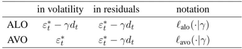
t for t = s+ 1, and the adjusted residuals εt, for t = s. Implementing the AVO adjustment therefore requires an extension to existing GARCH code. We summarise the adjustments needed to compute the modified log-likelihoods for the different outlier models in Table 1. We call these concentrated likelihoods, although the parameters of the model other than τ, only satisfy the first order conditions for MLE at one value ofγ.

Table 1: Adjustments for concentrated likelihood computation

in volatility in residuals notation ALO ε∗

t −γdt ε∗t −γdt `alo(·|γ)

AVO ε∗

t ε∗t −γdt `avo(·|γ) ε∗

t =yt−x0tζ,adjustments applied to log likelihood (2).

This adjustment avoids adding parameters of dummy variables to the log-likelihood which are difficult or impossible to estimate unrestrictedly.

In the first two motivating illustrations of our procedure, we use subsets of the weekly and monthly Dow Jones returns as discussed in more detail in §8. For the weekly data we use 574 observations

covering the years 1982 to 1992. The monthly data has 420 observations for the years 1965 to 1999. In both cases, a standard GARCH(1,1) with an intercept for the mean is estimated. Also in both cases, the largest outlier is found for the first observation after the Black Monday crash of 19 October 1987. This is the outlier candidate. Using the corresponding dummy variabledtin the mean, anddt−1in the

variance, the GAO model (11) is estimated next.

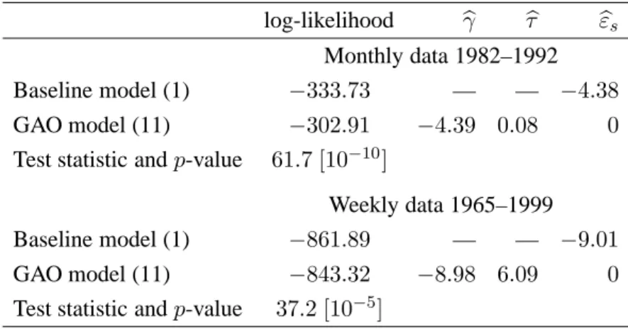
Table 2: Likelihood Ratio Testing for a generalized additive outlier (GAO) in Dow Jones returns log-likelihood γ_{b b}τ ε_bs

Monthly data 1982–1992

Baseline model (1) −333.73 — — −4.38

GAO model (11) −302.91 −4.39 0.08 0

Test statistic andp-value 61.7 [10−10_]

Weekly data 1965–1999

Baseline model (1) −861.89 — — −9.01

GAO model (11) −843.32 −8.98 6.09 0

Test statistic andp-value 37.2 [10−5_] Thessubscript refers to October 1987.

Table 2 gives the maximised log-likelihoods of the baseline GARCH(1,1) model and the GAO model. Thep-values of the likelihood ratio tests treat the timing of the outlier as unknown, i.e.sis considered as estimated from the data. They are based on an extreme value approximation discussed in§6 and Appendix A. In both data sets, the outlier candidate is highly significant.

−5.5 −5.0 −4.5 −4.0 −3.5 −305 −304 −303 Monthly γ→ AVO → log−likelihood ALO log−likelihood GAO log−likelihood AVO −12 −10 −8 −6 −850 −848 −846 −844 Weekly γ → ALO ↓ log−likelihood ALO log−likelihood GAO log−likelihood AVO

Figure 1: Likelihood grids of GAO, ALO, AVO models for GARCH(1,1) model of montly and weekly Dow Jones returns, as a function ofγ, the size of the October 1987 crash, see Table (1) for ALO and AVO concentrated likelihood computation. Note: GAO and AVO indistinguishable for weekly data.

Given the presence of an outlier att =s, we examine the outlier type. The decision on the type of additive outlier is based on`alo(·|bγgao)and`avo(·|bγgao), as discussed in Table 1. Figure 1 shows the concentrated likelihood grids as a function of the outlier sizeγ. The GAO model nests ALO and AVO, so always has a higher likelihood. The GAO grid can be computed from either`alo(·|γ)or`avo(·|γ)by adding the lagged dummy variable to the conditional variance equation and estimatingτ, conditional onγ. For the monthly data, ALO is very close to GAO: there is no significant difference using aχ2(1)

test. The likelihood of ALO is higher than AVO, and the former model is preferred. For the weekly data, Figure 1 shows the ALO likelihood to be bimodal, unlike the monthly case. Here, AVO and GAO are indistinguishable, so that the AVO model is preferred.

The procedure to decide between ALO and AVO is based on the likelihoods forγ_bgaoand therefore ignores the two global modes of the ALO model in case of bimodality. In practice it is possible that both ALO and AVO are significantly worse than the GAO model, although we have only encountered this very rarely. One approach to such a finding would be to adjust the GARCH likelihood in a similar manner as for ALO and AVO, so that a GAO correction can be imposed.

We conclude this section with a note on initialisation of the GARCH likelihood. In our computa-tions for the illustration of Figure 1 we conditioned on the first observation to initialize the GARCH recursion, so that the effective sample size is 419 and 573 respectively. Then, the value ofγ does not influence the likelihood of the observations prior tot=s. In the remainder of the paper, we use the sample mean ofε2t for initialization ofht, following the suggestion in Bollerslev (1986), which is more commonly followed in practice.

5

Detecting multiple outliers

The simplifying data adjustments and simplified likelihood-based tests are even more important when one suspects that more than one additive outlier of unknown type may be present: in that case a recursive detection procedure is required.

Based on the GAO model (11), we propose the following five step procedure to detect additive outliers in a GARCH(1,1) model:

Step 1 Estimate the baseline GARCH model (1), i.e. without any dummy variables, to obtain the

log-likelihood`bband residualsε∗t and volatilitiesh∗t.

Step 2 Find the largest standardized residual in absolute value,maxt|ε∗t/h∗t|. Denote this observa-tion by t = s. Estimate the GARCH GAO model (11) with dummy dt ≡ I(t = s) in the mean equation, anddt−1 in the variance equation (this can be done in most standard software

packages with GARCH estimation). This gives estimates for the added parameters _bγgao,s and b

τgao,srespectively, with log-likelihood`bgao,s.

Step 3 If 2(`bgao,s −`bb) < CTα then terminate: no new outlier is detected. Our approximation of the asymptotic distribution of this test under the null-hypothes of no outliers suggests that CT ≈ 5.66 + 1.88 logT at a significanceαof5%. The full approximation is given in§6.

Step 4 This step implements the AVO versus ALO selection, given that an outlier was detected:

(a) Ifτ_bgao,s<0then the outlier is of type ALO; else continue with step 4(b):

(b) Estimate the GARCH model with an ALO outlier correction of fixed size _bγgao,s. The model to be estimated corresponds to`alo(·|bγgao,s)from Table 1: it is a standard GARCH model without additional dummy parameters, but with a dependent variable that is cor-rected for the outlier, see§4. This model gives`balo,s.

(c) Estimate the GARCH model with an AVO outlier correction of fixed size bγgao,s. The model is`avo(·|bγgao,s)from Table 1, see§4 for its implementation. This gives`bavo,s. (d) If`bavo,s >`balo,s the outlier is AVO, else it is ALO.

The procedure can be iterated until no further outlier is detected. Because the outlier coefficients have already been estimated at each step, we propose to use the simple data correction of Table 1 when an outlier is detected. This data adjustment procedure avoids a proliferation of parameters in the log-likelihood.

Step 4 is used to distinguish between the two types of outliers, in case one is detected. It involves two additional GARCH model estimations, which can be initialised using estimates forα0, α1andβ1

from step 1, i.e. the baseline model (1) without any outlier effects. The same can be done in step 2, so that the additional overhead of the three maximum likelihood estimations is small.

Step 4(a) uses the fact that, because_bεs = 0for AVO:τ =α1γ2. Imposingα1 > 0shows that a

negativeτbis incompatible with the AVO model, saving the effort of estimating the model.

6

Controlling the size of the outlier detection procedure

We use extreme value theory, see e.g. Leadbetter, Lindgren, and Rootz´en (1983), and Monte Carlo simulation to determine an appropriate null distribution for the test in Step 3 of our outlier detection procedure of§5. Assuming that the single outlier test statistics are independent for alls, s= 1, . . . , T, and also that the dummy variable leading to the largest statistic is selected in Step 2, one can treat the test statistic in Step 3,

MT = max s∈(1,...,T)LR

GAO

T (s) = max

s∈(1,...,T)2(b`gao,s−b`b)

as the maximum of a random sample of size T from a χ2(2) distribution. Monte Carlo results in Appendix A show that the asymptoticχ2(2)approximation for a test for a single generalized additive outlier at a known fixed times, denoted byLRGAO_T (s), works well forT = 500.

Extreme value theory describes conditions under which MT follows an extreme value limit-ing distribution. These conditions do not require independence of the underlylimit-ing random variables LRGAO_T (s). In our case the limiting distribution is extreme value type I and the mean ofMT is a linear function of logT asT gets large. We use a response surface analysis of Monte Carlo experi-ments that leads to a good approximation of the finite sample distribution ofMT. The computation

of p-values and critical values only requires the knowledge of sample sizeT and does not require further simulation. Here we present the formula and the main simulation results; more detail is in Appendix A.

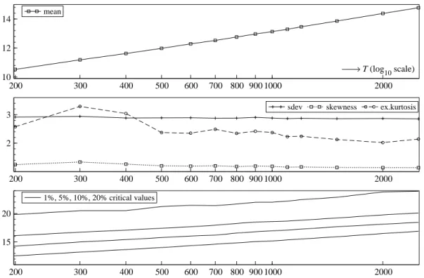
Steps 1–3 are simulated as described in§5 under the null hypothesis of no outlier. The Monte Carlo usesN = 10 000replications of the baseline model (1), a constant in the mean,xt = 1, ζ = 1and

α1 = 0.1, β1 = 0.8, α0 = 1−α1−β1. The sample sizes areT = 200(100)1200,1500,2000,2500.

The restrictions0<αb1+βb1 ≤1andαb0 >0are always imposed in the estimation procedure. The

results, shown in the first panel of Figure 2, indicate that the mean of the test statistic increases with the sample size, in proportion tologT asT → ∞, as predicted by extreme value theory. The variance, skewness and kurtosis are not very sensitive to the sample size, see the second panel of Figure 2. The last panel shows that the critical values are approximately equidistant, i.e. the critical value function, CV(α, T), is additively separable in two simple functions ofα and T and the distances between critical values of 20% and 10% on the one hand and between 10% and 5% on the other hand, are approximately equal. This is a characteristic of a Type I extreme value distribution.

200 300 400 500 600 700 800 900 1000 2000 10 12 14 → T (log₁₀ scale) mean 200 300 400 500 600 700 800 900 1000 2000 2

3 sdev skewness ex.kurtosis

200 300 400 500 600 700 800 900 1000 2000

15 20

1%, 5%, 10%, 20% critical values

Figure 2: Simulated moments (mean, standard deviation, skewness and excess kurtosis), and critical values (1%, 5%, 10%, 20%) of the maxsLR_TGAO(s)statistic under the null hypothesis.

Combining the extreme value Type I limiting distribution and the response surface analysis of Monte Carlo experiments in Appendix A, we form the following approximation for the distribution of the statisticMT, which we denote by maxsLR_TGAO(s):

P(maxsLRGAOT (s)≤x) = exp −exp −x+ 1.283−1.88 logT(1 + 12/T) 2.223 . (12)

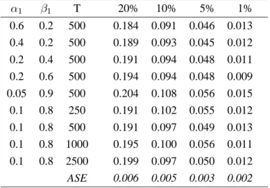
To check the accuracy of this approximation, we simulate the rejection frequencies for various parameter values under the null hypothesis. Table 3 lists the empirical size, showing that the procedure works well enough for practical use. The table also illustrates that the approximation works well for a range of GARCH parameters, indicating that the test is asymptotically similar with respect toα1and

β1.

Table 3: Size of (Max-)LR-test for single generalized additive outlier at unknown time

α1 β1 T 20% 10% 5% 1% 0.6 0.2 500 0.184 0.091 0.046 0.013 0.4 0.2 500 0.189 0.093 0.045 0.012 0.2 0.4 500 0.191 0.094 0.048 0.011 0.2 0.6 500 0.194 0.094 0.048 0.009 0.05 0.9 500 0.204 0.108 0.056 0.015 0.1 0.8 250 0.191 0.102 0.055 0.012 0.1 0.8 500 0.191 0.097 0.049 0.013 0.1 0.8 1000 0.195 0.100 0.056 0.011 0.1 0.8 2500 0.199 0.097 0.050 0.012 ASE 0.006 0.005 0.003 0.002 Based onN= 4 000replications.

ASE: Monte Carlo standard error of the rejection frequencies.

7

Power of the outlier detection procedure

Next, we investigate the performance of our procedure in detecting additive outliers, in selecting the type of additive outlier, and in determining the timing of the additive outlier. To investigate the power of the proposed test procedure by Monte Carlo, we selectT = 250, and have the DGP of type AVO as in (6) as well as of type ALO as in (4).1 The DGP parameters are set as α0 = 1−α1 −β1,

with γ = −3,−4,−5. The outlier enters near the middle of the sample: s = T /2. The results are presented in Table 4.

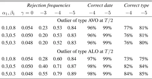
The first column in Table 4 gives the GARCH design parameters. The next four columns give the rejection frequencies at a 5%significance level. The results forγ = 0correspond to the size of the test, confirming a level close to5%. The remainder shows that the proposed procedure has satisfactory power to detect the outlier, regardless of the type of outlier. It is also remarkably good at detecting the date (i.e. the location) of the outlier, which, of course, is an important aspect of any detection procedure.2 _{Our procedure is also successful in detecting the type of outlier: there is no particular}

1

So we do not forceγto enter the DGP with the same sign as the drawn residual.

Table 4: Size and power of outlier detection test for a generalized additive outlier in a GARCH(1,1) model

Rejection frequencies Correct date Correct type

α1, β1 γ = 0 −3 −4 −5 −4 −5 −4 −5

Outlier of type AVO atT /2

0.1,0.8 0.054 0.23 0.53 0.84 96% 99% 77% 81%

0.3,0.5 0.050 0.20 0.53 0.83 96% 99% 76% 81%

0.5,0.3 0.048 0.20 0.52 0.83 96% 99% 76% 80%

Outlier of type ALO atT /2

0.1,0.8 0.054 0.28 0.60 0.84 97% 99% 73% 75%

0.3,0.5 0.050 0.40 0.71 0.87 98% 99% 82% 84%

0.5,0.3 0.048 0.55 0.79 0.89 98% 99% 84% 85%

Based on5%nominal rejection frequencies forN = 4 000andT = 250. Correct date: % with the correct date when an outlier was detected. Correct type: % with the correct outlier type when an outlier was detected.

Table 5: Samples for Dow Jones returns

frequency index at no. of observations scale

daily close of trade 29269 276

weekly midweek (or nearest day before) 5422 51

monthly end of month 1264 12

bias towards AVO or ALO, when an outlier is detected.

While the AVO results seem independent of the GARCH parameters, the power of ALO appears to increase asα1increases. The likely explanation is that this corresponds to a larger volatility effect

when left unmodelled, see equation (8) above. Overall, the proposed outlier detection procedure works very well, even at this small sample size where GARCH models can be somewhat harder to estimate. Essentially the same results were obtained for a sample size of 500.

8

Multiple outlier applications for Dow Jones returns

As an application of the new outlier-detection procedure we consider the returns on the Dow Jones Industrial Average index,3 using monthly, weekly, and daily data for the period 1896, May 26, to 2001, December 5. Table 5 provides some details.

The return data are formed by taking the first difference of the logarithms and then annualized. These returns were multiplied by the scale factor given in Table 5, selected as the integer which made the annualized average return for the daily and weekly returns as close as possible to the average for the monthly data.

Visual inspection of the daily returns shows the largest drop in 1914, followed closely by 1987. In 1914, the exchange was closed for four and a half months following the outbreak of World War I. So there is a long period of missing data in 1914 (during that period, grey trading continued outside the exchange). The year 1929 is characterized by boom and bust, followed by a period of long decline, and is historically the period with the highest volatility. October 1987 saw the largest one-day drop in the index, but it took less than two years to reach the pre-crash levels again. The last sharp fall followed the 11 September 2001 terrorist attacks on Washington and New York, which is indicated as an outlier in the daily data.

Table 6: Detected outliers in GARCH(1,1) model for monthly and weekly Dow Jones returns 1896-2001.

date size p-outlier p-AVO p-ALO type monthly returns: 12∆ logym

t 1987/10 −4.39 0.083 τ <b 0 0.795 ALO 1914/12 −3.58 0.00012 0.478 0.112 AVO 1940/05 −3.11 0.00022 τ <b 0 0.241 ALO 1937/09 −2.37 0.028 0.122 0.001 AVO 2001/09 0.129 —

weekly returns: 51∆ logyw t 1914/12/16 −16.75 0 0.042 0.244 ALO 1940/05/15 −7.05 0 1 0 AVO 1899/12/13 −7.14 0.083 0.206 0.026 AVO 1987/10/21 −8.95 0.053 0.287 0.010 AVO 1926/03/03 −4.84 0.00015 1 0.002 AVO 1898/05/11 7.61 0.00020 0.030 0.960 ALO 1994/03/30 −3.39 0.00075 0.120 0.536 ALO 1998/09/02 0.070 —

p-outlier is for testing no outlier against a GAO at an unknown date.

p-ALO is for testing ALO against GAO, conditional on a known outlier date.

p-AVO is for testing AVO against GAO, conditional on a known outlier date. Notation:0.045 = 0.00005

We apply our outlier detection procedure recursively: first detect the largest outlier, then adjust for this as discussed in§4, next, detect and adjust for the subsequent outlier, until no more are found. This

approach is along the lines of Chen and Liu (1993), and therefore susceptible to the same criticism that estimates of the other model parameters, in particular α0, are contaminated by the presence of

an outlier. Robust estimation of GARCH models is possible, but rather costly and difficult to imple-ment, see Sakata and White (1998) and therefore not yet attractive. The problem can be mitigated by applying a Studentt-error distribution, see§9.2 below.

The top half of Table 6 lists the results when applying the procedure to the monthly data. The column labelled p-outlier gives the p-value of the test for a generalized additive outlier, based on the extreme value approximation. Detected are the 1987 crash, the start of the two world wars in Western Europe, as well as September 1937 (when the index dropped by 17%). The order in the table follows the order in which the outliers were detected, and we also include the first outlier with a p-value>5%. The column labelledp-AVO reports thep-value for theχ2_{(1)likelihood-ratio test of}

the AVO restriction within the GAO model. Similarly, the next column has the test outcome for the ALO restriction. Note that AVO is rejected without further testing, whenτ <_b 0, according to Step 4a of the procedure. In December 1914, when the stock market reopened, both ALO and AVO are not significantly different from GAO. However, the likelihood of AVO is higher than ALO, so the former is selected.

The second part of Table 6 gives the results for the weekly data. We see more AVO outliers, as expected. At different frequencies, the pattern of outliers will also be different: a brief crash or rally within a month can be hidden by only looking at the end-of-month data. The world wars are now the largest outliers, and World War II is detected as an AVO. Also, the13%fall in the second week of December 1899 is detected before the 1987 crash. Except for the final outlier in 1994, the ALO versus AVO decision is clear-cut.

In Table 7 we list the dates of outliers for the daily model, but this time in chronological order. There are more than five times as many observations as in the monthly data set, but also five times as many outliers. The procedure is found to be acceptably fast on the daily data, taking less than half an hour for nearly30 000 observations (on a 800 Mhz Pentium III notebook; this includes the first estimation).

The results in this section assume that the underlying model is Gaussian GARCH(1,1), possibly contaminated with outliers. Outliers only exist with reference to a model, and using the wrong model could lead to the detection of too many outliers. Especially for the daily data, it may be that the GARCH model with student-tdistributed errors, which is readily available in standard software, is a better description. This is explored in the next section.

9

Extensions to other models

9.1 GARCH(2,2) models

In the GARCH(p, q) case, the lag polynomialα(L)in (10) hasqterms instead of one. The equivalent extension to the equation forhtin the GAO model (11) would be to add the dummy variable with lags

Table 7: Detected outliers using the new procedure in GARCH(1,1) model for daily Dow Jones re-turns: 276∆ logyd

t

date type p-outlier date type p-outlier date type p-outlier 1899/12/08 AVO 0.043 1924/02/15 AVO 0.0037 1950/06/26 AVO 0.066

1901/05/08 AVO 0.0008 1925/11/10 AVO 0.0015 1955/09/26 AVO 0

1901/09/07 AVO 0.0208 1927/10/08 AVO 0.0325 1962/05/28 AVO 0.0039

1904/12/07 AVO 0.045 1929/10/28 AVO 0.0002 1982/08/17 AVO 0.0055

1907/03/14 AVO 0.0005 1933/03/15 ALO 0.048 1986/09/11 ALO 0.0033

1913/01/20 ALO 0.066 1934/07/26 ALO 0.0067 1987/10/19 AVO 0

1914/07/28 ALO 0.045 1939/09/05 ALO 0.0031 1989/10/13 AVO 0

1914/07/30 AVO 0.043 1940/05/13 AVO 0.063 1991/01/17 ALO 0.0158

1914/12/12 ALO 0 1943/04/09 ALO 0.0004 1991/11/15 AVO 0.063

1916/12/12 AVO 0.0012 1946/09/03 AVO 0.0034 1997/10/27 AVO 0.042

1917/02/01 ALO 0.061 1948/11/03 AVO 0.048 2000/04/14 ALO 0.0156

2001/09/17 AVO 0.0002

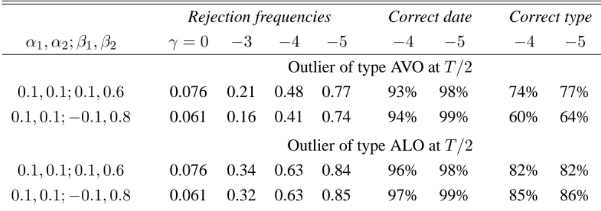
1 toq as the variance equation is affected by a level outlier forqperiods. As a simple alternative we do not extend the GAO model with extra lags of the dummy variable. Instead, we just apply the same procedure as for GARCH(1,1), introducing only one dummy variable in the variance equation and leaving the approximation to the distribution of the test statistic in Step 3 unchanged. We evaluate our test procedure by Monte Carlo for 16 different GARCH(2,2) data generating processes both with and without additive outliers. The results in Table 8 show that the size and power are very close to that in the GARCH(1,1) case. However, the procedure detects more additive level outliers in Step 4, which could be caused by the omission of the additional lagged dummies, together and the rule 4a thatbτ <0

corresponds to an ALO.

9.2 GARCH-t _{models and effects of outlier correction on GARCH parameter}

esti-mates

A GARCH model with Student-tdistributed errors, as proposed by Bollerslev (1987), is a likely al-ternative for a GARCH model with additive volatility outliers. Appendix A discusses the adjustments that we made to the extreme value approximation when incorporating the standardized t(ν) distribu-tion. As the form of the limiting extreme value distribution is nonstandard in this case and depends on the unknown ν, our approximation does not work as well as in the Gaussian model. Table 9 presents some results for the test. As expected, the actual outliers have to be considerably larger to be distinguished from the thick tail of the Student-t(6)distribution.

Table 8: Size and power of the test for a generalized additive outlier at unknown time in a GARCH(2,2) model

Rejection frequencies Correct date Correct type

α1, α2;β1, β2 γ = 0 −3 −4 −5 −4 −5 −4 −5

Outlier of type AVO atT /2

0.1,0.1; 0.1,0.6 0.076 0.21 0.48 0.77 93% 98% 74% 77%

0.1,0.1;−0.1,0.8 0.061 0.16 0.41 0.74 94% 99% 60% 64% Outlier of type ALO atT /2

0.1,0.1; 0.1,0.6 0.076 0.34 0.63 0.84 96% 98% 82% 82%

0.1,0.1;−0.1,0.8 0.061 0.32 0.63 0.85 97% 99% 85% 86% 5%nominal rejection frequencies forN = 2 000,T = 500.

Correct date, type: % correct when an outlier was detected.

Table 9: Size and power of the test for a single generalized additive outlier at unknown time in a GARCH(1,1)-t(6)model,α1 = 0.1, β1 = 0.8

Rejection frequencies Correct date Correct type

γ = 0 −5 −8 −10 −15 −8 −10 −15 −8 −10 −15

Outlier of type AVO atT /2

0.043 0.04 0.08 0.22 0.74 92% 98% 99% 77% 84% 96%

Outlier of type ALO atT /2

0.043 0.05 0.26 0.48 0.84 91% 96% 99% 90% 95% 96%

Based on5%nominal rejection frequencies forN = 2 000andT = 1 000. Correct date, type: % correct when an outlier was detected.

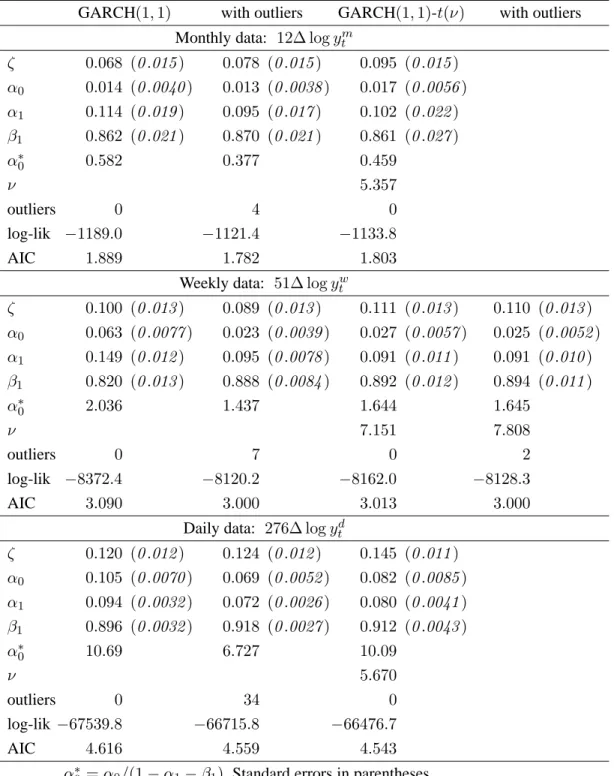
Empirical application to the Dow Jones industrial averages index supports the closeness of the Gaussian GARCH(1,1) model with generalized additive outliers and the GARCH(1,1)-tmodel. Ta-ble 10 shows that at the monthly and weekly level, the two models seem to be close substitutes, with the outlier model weakly preferred on AIC, where we treat the date and type of the outlier as known and count the sizes of the outliers as extra parameters to be estimated. At the daily level, the GARCH-tis preferred, yielding a higher log-likelihood and lower AIC than the model with outliers. Both the outlier extension and the introduction of tdistributed errors significantly affect the estimates for the GARCH parameters in the weekly and daily data: α_b0 and αb1 increase, βb1 decreases. The ’robust’

estimation of the mean return using the Student-errors significantly increasesζb(the intercept) as the predominantly negative returns receive a lower weight. A similar effect was observed by Sakata and White (1998) for daily S&P 500 returns (1987/8-1991/8) when they applied robust high breakdown

estimators for the GARCH(1,1) model. The outlier correction does not have a significant impact on the estimated mean return as the percentage of outliers is very small.

Table 10: Estimated GARCH(1,1) coefficients for Dow Jones returns at various frequencies

GARCH(1,1) with outliers GARCH(1,1)-t(ν) with outliers Monthly data: 12∆ logytm

ζ 0.068 (0.015) 0.078 (0.015) 0.095 (0.015) α0 0.014 (0.0040) 0.013 (0.0038) 0.017 (0.0056) α1 0.114 (0.019) 0.095 (0.017) 0.102 (0.022) β1 0.862 (0.021) 0.870 (0.021) 0.861 (0.027) α∗ 0 0.582 0.377 0.459 ν 5.357 outliers 0 4 0 log-lik −1189.0 −1121.4 −1133.8 AIC 1.889 1.782 1.803

Weekly data: 51∆ logywt

ζ 0.100 (0.013) 0.089 (0.013) 0.111 (0.013) 0.110 (0.013) α0 0.063 (0.0077) 0.023 (0.0039) 0.027 (0.0057) 0.025 (0.0052) α1 0.149 (0.012) 0.095 (0.0078) 0.091 (0.011) 0.091 (0.010) β1 0.820 (0.013) 0.888 (0.0084) 0.892 (0.012) 0.894 (0.011) α∗ 0 2.036 1.437 1.644 1.645 ν 7.151 7.808 outliers 0 7 0 2 log-lik −8372.4 −8120.2 −8162.0 −8128.3 AIC 3.090 3.000 3.013 3.000

Daily data: 276∆ logy_td

ζ 0.120 (0.012) 0.124 (0.012) 0.145 (0.011) α0 0.105 (0.0070) 0.069 (0.0052) 0.082 (0.0085) α1 0.094 (0.0032) 0.072 (0.0026) 0.080 (0.0041) β1 0.896 (0.0032) 0.918 (0.0027) 0.912 (0.0043) α∗ 0 10.69 6.727 10.09 ν 5.670 outliers 0 34 0 log-lik −67539.8 −66715.8 −66476.7 AIC 4.616 4.559 4.543 α∗

For each frequency we also applied the GARCH-toutlier test to the GARCH-tmodels. Only for the weekly data were outliers detected: ALO when the market reopened after World War I, and AVO at the start of World War II. These are the same two leading outliers found in the normal GARCH(1,1) model. However, in terms of AIC the GARCH-tmodel with outliers is not an improvement over the normal GARCH(1,1) model with outliers. The effect of the outliers detection on the estimated ν is small. For the monthly data, the closest candidate outlier in the GARCH-tmodel was October 1987, with ap-value of0.052. In daily data, the closest candidate was September 26, 1955, which was also the first one found in the GARCH(1,1) model, but now withp-value of0.10rather than zero.

10

Conclusion

We introduced a new detection procedure for additive outliers in GARCH models. This procedure has several advantages over existing procedures:

• It is simple to implement and contains a convenient procedure to compute p-values for tests, without the need for simulation.

• It is likelihood-based and associated tests are asymptotically similar with respect to the GARCH parametersα1andβ1.

• Simple nested tests distinguish between Additive Level Outliers and Additive Volatility Out-liers.

• The procedure can be extended to other types of GARCH models such as EGARCH, etc. Our applications on monthly, weekly and daily Dow Jones returns show that the test procedure also works well in practice. We compare estimates of our outlier model with a GARCH-tmodel, also possibly affected by outliers. The GARCH-tmodel without outliers is to be preferred over the normal GARCH with outliers for the daily Dow Jones returns.

Other practical aspects of the procedure could be examined. Although the in-sample fit of a GARCH-tand normal-GARCH with outliers for the monthly Dow Jones returns may be quite simi-lar, the forecasted volatility will be quite different. It may be that the former is preferred in practice, for example for value-at-risk estimations. Conclusions regarding leverage effects in the form of asym-metric volatility could be also different: the outlier detection, for the data considered, predominantly removes negative shocks.

The proposed method could become a useful addition to the toolkit of empirical volatility mod-ellers. The first-step outlier test can serve as a mis-specification test for the model. Next, the iterated procedure can be used as a robustification of the model (with too many outliers suggesting that the model is inadequate). Finally, the detected outliers can complement value-at-risk estimations: in large samples, the distribution of outliers is informative in itself, otherwise the estimates may require their absence.

Acknowledgements

We wish to thank Siem Jan Koopman for helpful discussions and suggestions. We’d also like to thank Dayong Zhang for reporting some errors in earlier versions of the paper. Financial support from the UK ESRC (grant R000237500) is gratefully acknowledged by JAD. JAD would also like to thank the Graduate School of Business at Stanford University for their hospitality while writing the first version. The computations were performed using the Ox programming language (Doornik, 2001).

References

Abraham, B. and N. Yatawara (1988). A score test for detection of time series outliers. Journal of Time Series Analysis 9(2), 109–119.

Bollerslev, T. (1986). Generalised autoregressive conditional heteroskedasticity. Journal of Econometrics 51, 307–327.

Bollerslev, T. (1987). A conditional heteroskedastic time series model for speculative prices and rates of return. Review of Economics and Statistics 69, 542–47.

Bollerslev, T., R. F. Engle, and D. B. Nelson (1994). ARCH models. In R. F. Engle and D. L. McFadden (Eds.), Handbook of Econometrics, Volume 4, Chapter 49, pp. 2959–3038. Amsterdam: North-Holland. Chen, C. and L. M. Liu (1993). Joint estimation of model parameters and outlier effects in time series.

Journal of the American Statistical Association 88, 284–297.

Doornik, J. A. (2001). Object-Oriented Matrix Programming using Ox (4th ed.). London: Timberlake Con-sultants Press.

Doornik, J. A. and M. Ooms (2000). Multimodality in the GARCH regression model. mimeo, Nuffield College.

Engle, R. F. (1982). Autoregressive conditional heteroscedasticity, with estimates of the variance of United Kingdom inflation. Econometrica 50, 987–1007.

Franses, P. H. and D. van Dijk (2000). Outlier detection in GARCH models. Econometric Institute Report EI-9926/RV, Erasmus University Rotterdam.

Gourieroux, C. (1997). ARCH Models and Financial Applications. New York: Springer Verlag.

Hotta, L. K. and R. S. Tsay (1998). Outliers in GARCH processes. mimeo, IMECC, Brazil and University of Chicago.

Leadbetter, M. R., G. Lindgren, and H. Rootz´en (1983). Extremes and Related Properties of Random Se-quences and Processes. Springer Series in Statistics. Springer-Verlag, New York, Heidelberg, Berlin. Mood, A. M., F. A. Graybill, and D. C. Boes (1974). Introduction to the Theory of Statistics, Third Edition.

McGraw-Hill.

Sakata, S. and H. White (1998). High breakdown point conditional dispersion estimation with application to s&p 500 daily returns volatility. Econometrica 66, 529–567.

Shephard, N. (1996). Statistical aspects of ARCH and stochastic volatility. In D. R. Cox, D. V. Hinkley, and O. E. Barndorff-Nielsen (Eds.), Time Series Models in Econometrics, Finance and Other Fields, pp. 1–67. London: Chapman & Hall.

A

Approximating the distribution of the max

s

LR

GAO_T

(

s

)

test

This appendix describes the details of the experiments leading to the approximation for the maxsLRGAO T (s) test in the normal case described in §6. We also present adjustments to the approximation for the case of Student-terrors, that we discuss in§9. In order to simplify the presentation we denoteLRGAO_(s)byX

sand maxsLRGAO

T (s)byMT.

The single likelihood-ratio test for a Generalized Additive Outlier at a known timet = s, denoted by

LRGAO_{(s), involves two parameters that are well identified under the null, giving the test statistic an asymptotic}

χ2_{(2)≡exp(1/2)distribution. The effectiveness of this asymptotic approximation for a sample size of 500 is} illustrated below.

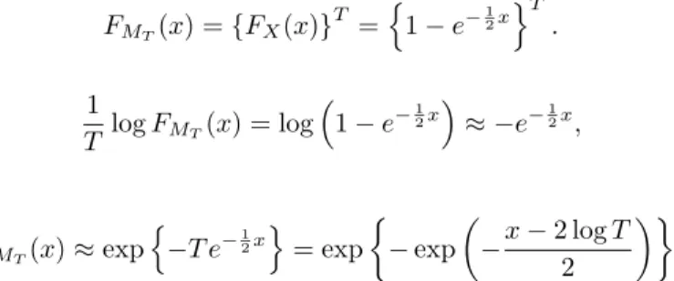
As we effectively do T such tests we wish to approximate the distribution of the maximum: MT = max(X1, . . . , XT). Assuming independently and identically distributedXsthe cumulative distribution func-tionFMT ofMT is given by FMT(x) ={FX(x)} T =n1−e−12x oT . Using 1 T logFMT(x) = log 1−e−12x ≈ −e−12x,

whenxis large, gives

FMT(x)≈exp n −T e−12x o = exp −exp −x−2 logT 2 ,

such that for largexand largeT,MT has a Type I extreme value limiting distribution. Our approximations are based on this distribution type. Leadbetter, Lindgren, and Rootz´en (1983, Chapters 1,3) show that Type I extreme value (or Gumbel-) limiting distributions apply much more generally. TheXsneed not be exponential and independent, although these are the cases where the asymptotic theory works well, also in moderately sized samples. In general, when FMT(x) = exp −exp −x−aT b , (13)

the expectation and variance ofMT are given byE[MT] ≡ mT = aT +δb, where δ ≈ 0.577216, and V[MT] =b2π2/6, see e.g. Mood, Graybill, and Boes (1974, Appendix B). Critical values at significance level

αcan therefore be computed as

CTα=−blog(−log(1−α)) +aT. (14) Although theXsare not independently distributed in our case, we can use the extreme value distribution (13) as the limiting distribution. TheXsare not fat tailed and they are short memory under the null hypothesis of no outliers, so the required distributional mixing conditions for a Type I extreme value distribution are met, see Leadbetter, Lindgren, and Rootz´en (1983, Ch. 3). The general theory allows the variance of the approximating distribution, and thereforeb, to depend onT. This does not apply to our statistic.

Simulating the distribution ofMT for increasing sample sizesT, as reported in§6, we observe that the simulated standard deviation,V[WT]1/2, of the test statistic is close to constant. Its asymptotic value is2.851 with standard error0.008, found from a regression on a constant,T−1_andT−2_{. This results in}b_{b= 2.223.}

After some experimentation, we found that the means from the Monte Carlo experiment in§6, depicted as 14 observations in the upper panel of Fig. 2, are very well described by the following regression:

b mTi = 1.880 (0.0013) log(Ti) + 22.7 (1.2) log(Ti)/Ti, i= 1, . . . ,14,

where heteroscedasticity consistent standard errors (HCSE) are given in parentheses. The residual normality test of this regression insignificant, but there is significant heteroscedasticity. The intercept is insignificant. The resulting response surface formT, bas a function of sample sizeT is:

aT = mT −δb ≈1.88 logT(1 + 12/T)−1.283,

b ≈ 2.223. (15)

Because the number of Monte Carlo experiments is quite big, we have a large number of draws from the (hypothesized) extreme value distribution. This in turns leads to accurate estimates of the mean and standard deviation, for which we adopted the method of moments to determine the parameters of the limiting distribution. We could instead have used the disaggregated data along the lines of, e.g., Tsay, 2002, §7.5.2.1, to directly estimateaT andbT. This would give very similar outcomes for the resulting critical values, but with better estimates of the overall parameter uncertainty in the approximation at varying levels ofT.

Abraham and Yatawara (1988) (AY88) use a similar extreme value approximation for the maximum of a sequence ofχ2_{(2)distributed LM tests for time series model outliers. They do not fit equations for the moments} of the extreme value distribution, but instead adjust the critical value approximation (14), with fixedb= 2and derive a constant term in the critical value equation,log(θ), using Monte Carlo Simulations.

(AY88) :CTα=−2 log(−log(1−α)) + 2 log(T) + log(θ) (16) withT the number of (dependent) outlier tests. They estimated an extremal indexθ = 0.8. The termlog(θ) corrects the critical values for the dependence of the test statistics, see Leadbetter, Lindgren, and Rootz´en (1983, p.67) for a formal definition. θ= 1for (asymptotically) independent statistics. Abraham and Yatawara (1988) also note that applying the test with estimated parameters for the time series model, rather than using known parameters markedly decreases the empirical critical values for the test. A similar effect may explain that the coefficient oflog(T)is lower than two in our approximation formula (15). The specification (16) would work badly in our case.

200 300 400 500 600 700 800 9001000 2000 12.5 15.0 17.5 20.0 22.5 → T (log₁₀ scale) 1% 5% 10% 20%

1%, 5%, 10%, 20% simulated critical values 1%, 5%, 10%, 20% fitted critical values

Figure 3: Simulated and fitted critical values (1%, 5%, 10%, 20%) of the maxsLRGAOT (s)test statistic under the null hypothesis.

Next, we turn to the case with a Student-terror term. We first note thatMTof a sample oft(ν)-distributed variables has a type II extreme value (Fr´echet) limiting distribution:

FMT(x) = exp

−x−ν _{, (17)}

whereν, the tail index, determines the shape of the distribution. Thek-th moments ofMT are now given by E[Mk

T] = Γ(1−k/θ), whereΓis the gamma function. In this caseν equals the degrees of freedom of the Student distribution, see Mood, Graybill, and Boes (1974,§6.5.3, example 12).

As theLRGAO _{test involves the test for a single outlier in a GARCH-tmodel, one may perhaps expect} that the type II behaviour also applies here. It may also be that the type I approximation is still reasonable for common values ofν.

In order to investigate this issue we compare the distributions of theLRGAO_{(s)test for a fixedsin the cases} of normal errors and Student-terrors using simulation. Figure 4 presents QQ plots of the simulation results for the design given in§6 forT = 500andN = 10000, testing for an outlier at the middle of the sample:s=T /2. The solid line in Figure 4 makes clear that the distribution for theLRGAO_{test for an outlier at a known point} in a GARCH model with normal errors is indeed close toχ2_(2).

Note that for Student-t(6)errors, the distribution ofLRGAO_{is considerably more spread towards the right} tail. At first sight, this may indicate that a type I extreme value distribution does not apply here. However, if we simulate the critical values of the maxsLRGAOT (s)test under Student-terrors, the distribution of the

0 1 2 3 4 5 6 7 8 9 10 11 12 5

10 15

GARCH GARCH−t(6)

Figure 4: QQ plot against aχ2(2)reference distribution of the LR(2) test for an outlier in the middle of the sample: normal GARCH(1,1) (solid line) versus GARCH-t(1,1) with t(6)errors. T = 500, N = 10 000. 200 300 400 500 600 700 800 9001000 2000 12.5 15.0 17.5 ν=∞ ν=13ν=9 ν=6 ν=5 ν=4 mean 200 300 400 500 600 700 800 9001000 2000 3.0 3.5 4.0 ν=4 ν=5 ν=6 ν=9 ν=13 ν=∞ standard deviation

Figure 5: Simulated moments (mean, standard deviation), of the maxsLRGAOT (s) statistic in a GARCH-t(ν)(1,1) under the null hypothesis, forν= 4,5,6,9,13and∞(normal).

test shifts withν, but the distance between critical values at 5% and 10% and between 10% and 20% for a specificν remain very close, as in Figure 2. Figure 6 presents simulated critical values for Student-terrors. The differences in critical values for a type II extreme value distribution are determined by[−log(1−α)]−1/ν

which should not lead to an equal spacing between 5% and 10 % and 10% and 20% critical values. This is an indication that that the type II approximation would not work well here.

Instead of using a type II approximation, we adapt the type I extreme value approximation under normal errors to the Student-t(ν)case by allowingmT andbto depend onν. Based on GARCH(1,1)-t(ν)Monte Carlo simulations forν= 4,5,6,9,13, the following adjustments can be used to approximate the distributions for the

outlier test in the GARCH(1,1)-t(ν)model:

m(T, ν) ≈ mT + 11ν−1+ 0.25mTν−1/2,

b(ν) ≈ b+ 12ν−2_, (18)

withmT andbgiven in (15). We did not allowbto depend onT, although the simulations show the variance to be somewhat u-shaped forνranging from4to6. The response surface for the mean fits remarkably well. The approximation to the critical values is satisfactory, see Figure 6, except whenν = 4, and to a lesser extent for

ν = 5at1%. 200 300 400 500 1000 2000 15.0 17.5 20.0 22.5

20% simulated critical values fitted 200 300 400 1000 2000 17.5 20.0 22.5 ν=4 5 6 9 13 10% simulated critical values

fitted

200 300 400 1000 2000

20.0 22.5 25.0

5% simulated critical values fitted 200 300 400 1000 2000 22.5 25.0 27.5 30.0

1% simulated critical values fitted

Figure 6: Simulated and fitted critical values (1%, 5%, 10%, 20%) of the test statistic for GAO in GARCH-t(ν) under the null hypothesis.

B

Alternative outlier detection procedures for GARCH(1,1) models

We discuss to alternative approaches. Hotta and Tsay (1998) built a procedure based on LM tests. Franses and van Dijk (2000) suggested a procedure based on regressions.

B.1 Additive volatility outliers

Hotta and Tsay (1998) propose an LM test on the largest standardized residual: LMAVO= max 1<t<T b ε2 t b ht .

This is approximately distributed as the maximum of a random sample of sizeT−2from aχ2_{(1)distribution.}

B.2 Additive level outliers

Hotta and Tsay (1998) propose an LM test for the ALO case:

LMALO= max 1<t<T b ε2 t b ht n 1 +α_b1bhtPJj=t+1βb j−(t+1) 1 bh−j2 b hj−εb2j o2 1 + 2αb2 1bh2t PJ j=t+1βb 2[j−(t+1)] 1 bh− 2 j .

t < J ≤ T is a truncation parameter that is introduced to avoid ‘swamping’. The distribution of LMALO depends on the choice ofJ, and the true values ofα1andβ1, requiring simulation for every test. Finally, they suggest, when both LMALOand LMAVOare significant, to adopt the one with the most significant value. The

p-values of LMALOcan only be obtained by simulation, which can hinder the decision between outlier types: if the AVO test has a very smallp-value, many replications are required to decide whether the ALO test has an even smallerp-value or not. Moreover, there is no guarantee that the candidate outliers for both tests occur at the same observation.

Franses and van Dijk (2000) suggest the following procedure for detecting additive level outliers in GARCH(1,1) models. Using the ’variance innovations’ut=ε2t−htandu∗t =ε∗t2−h∗t they rewrite (8) as (so this is under the impact of a neglected outlier):

u∗

t =φ

I(t=s)−α1β1t−s−1I(t > s) +ut,

whereφ = 2γεs+γ2 is the direct impact of the outlier on the sequence of variance innovations. Theφ parameter is estimated by regression ofu_b∗

t = bε∗t2−bh∗t on n

I(t=s)−αb1βb1t−s−1I(t > s) o

, whereα_bandβb

are obtained in the baseline GARCH(1,1) model. From this they solve forγ:

b γs=          0 if_bε∗2 s −φ <b 0, b ε∗ s− b ε∗2 s −φb 1/2 if_bε∗2 s −φb≥0andεb∗s≥0, b ε∗ s+ b ε∗2 s −φb 1/2 if_bε∗2 s −φb≥0andεb∗s<0.

The largest_bγsexceeding a certain critical value is used to remove the outlier from the data. An approximation for the critical value is offered for certain significance levels. If an outlier is found, att0say, the procedure is repeated foryt−γct0I(t = t0)until no further outliers are detected. This procedure could be combined

with LMAVOalong the lines suggested by Hotta and Tsay (1998) (i.e. selecting the outcome with the smallest

p-value). In both cases, the assumption is that the outlier is of the same sign as the observed residual. In addition, Franses and van Dijk (2000) select the smallest solution (in absolute value). Although this provides a unique choice forγ, their regression method for the variance innovations often suggests the existence of multiple solutions forγ, even when these are not indicated by the log-likelihood. See, e.g., the left hand side likelihood grid in Figure 1.

Both the LM based approach and the regression procedure are rather complex, and suffer from non-similarity with respect to the GARCH parameters, so that new simulations are needed to computep-values in each empirical application.

B.3 Simulation comparison

Next, we contrast our procedure to these alternative methods, denoted FD for the regression procedure of Franses and van Dijk (2000), and HT for the LM test based approach of Hotta and Tsay (1998). The results are in Table 11.4 _{The main findings are that FD, although not designed to test for AVO, it will have some power} against it; FD has lower power than HT when the outlier is of type ALO, probably because HT actually uses two tests (a more appropriate comparison would be with LMALOonly). HT and our procedure have similar power, but the latter is much better at dating the outlier. Surprisingly, HT is worse at dating for the larger outliers as the LM tests lose their optimal power properties for distant alternatives. In addition, our procedure is more successful in classifying the outlier.

Table 11: Size and power of outlier detection tests for a single outlier in a GARCH(1,1) model Rejection frequencies Correct date Correct type

α1, β1 γ = 0 −4 −5 −4 −5 −4 −5

Outlier of type AVO atT /2

HT 0.1,0.8 0.047 0.55 0.84 97% 96% 50% 39%

HT 0.3,0.5 0.044 0.54 0.85 82% 75% 54% 48%

HT 0.5,0.3 0.045 0.54 0.85 70% 66% 60% 56%

Outlier of type ALO atT /2

FD 0.1,0.8 0.050 0.45 0.73 91% 97% FD 0.3,0.5 0.042 0.30 0.55 82% 91% FD 0.5,0.3 0.075 0.27 0.50 72% 85% HT 0.1,0.8 0.047 0.58 0.82 97% 96% 75% 80% HT 0.3,0.5 0.044 0.69 0.85 88% 78% 75% 81% HT 0.5,0.3 0.045 0.76 0.86 72% 56% 60% 75%

HT is LM approach of Hotta and Tsay (1998); FD is regression method of Franses and van Dijk (2000). For further notes: see Table 4.

B.4 Application Comparison for the Dow Jones returns

Table 12 lists the results when applying the three procedures to the monthly Dow Jones returns. The order in the table is that in which the outliers were detected, and we also include the first outlier with ap-value>5%.

The procedure of Hotta and Tsay (1998) finds the same outliers as our method, with two additional ones. Note that Hotta and Tsay (1998) use simulation to determinep-values for the ALO test. For large outliers, the result is ap-value of zero, because it would be too time consuming to find accurate values (we use1000 replications andJ = 3). In our implementation, ALO is selected over AVO in that situation.

Franses and van Dijk (2000)’s procedure only detects ALO, which is less of a problem with monthly data, nonetheless giving quite different results. This method was the only to detect a positive outlier in the monthly data: August 1932 saw a large upswing in the index. The size of the first detected outlier is rather different from the other methods, as the multiple solution forγsuggested by their regression for the variance innovations did not arise in the other methods.

This could also explain the subsequent differences in the detection path. For the weekly and daily results we exclude this method, because it would need to be combined with an AVO detection (adding LMAVOis simple, but does require simulation to determinep-values). The consequence of only correcting for ALO in the weekly returns is that about twice as many outliers are found, often close to each other. This illustrates the advantages of implementing volatility outliers.

4_{To compute the rejection frequency, we used the extreme value approximation (12) for our procedure. For HT we used}

simulation based on1000replications andJ = 3. For FD we use the given critical value approximation, except that we replaceκwithmax(3, κ). This is not a good solution, though, e.g. whenα= 0.6andβ= 0.2, we would use the value 3, but simulations find a size of20%in that case.

Table 12: Detected outliers in GARCH(1,1) model for monthly Dow Jones returns: 12∆ logym t new procedure

date type size p-outlier p-ALO 1987/10 ALO −4.38 0.083 0.795

1914/12 ALO −3.58 0.00012 0.112

1940/05 ALO −3.11 0.00018 0.251

1937/09 AVO −2.37 0.036 0.002

2001/09 — 0.139

Hotta and Tsay (1998)

date type size p-LMAVO p-LMALO 1987/10 ALO −4.38 0.074 0 1914/12 ALO −3.58 0.045 0 1940/05 ALO −3.11 0.008 0.002 1899/12 ALO −2.49 0.039∗ _0.025 1937/09 AVO −2.38 0.0457 0.046∗ 1990/08 ALO −1.79 0.052∗ 0.043 2001/09 — 0.053 0.069∗∗

Franses and van Dijk (2000) date type size

1987/10 ALO −3.78

1932/08 ALO +3.44

1940/05 ALO −2.54

1914/12 ALO −2.76

p-ALO is for testing ALO, when an outlier is detected.

∗_{at date of subsequent outlier candidate;}∗∗_{at 1907/3.}

Notation:0.045 = 0.00005

Table 13 gives the results for the weekly data. Four out of the seven outliers that are found by both our procedure and HT are now of a different type. The HT procedure detects two more outliers albeit atp-values that are not very low.

The application comparison shows two clear benefits of our new procedure: it is a nested procedure, avoid-ing the need to have to comparep-values of two separate tests, possibly at different dates. It is also easy to computep-values at the second stage, allowing for better classification in ALO and AVO.

The new procedure is found to be considerably faster on the daily data, taking less than half an hour for nearly30 000observations (on a 800 Mhz Pentium III notebook; this includes the first estimation). HT takes two and a half hours, requiring simulation, and FD more than seven hours. FD requires nearly30 000regressions for each test, but there is scope for implementing this more efficiently.

Table 13: Detected outliers in GARCH(1,1) model for weekly Dow Jones returns:51∆ logytw new procedure

date type p-outlier p-ALO size

1914/12/16 ALO 0 0.244 −16.75 1940/05/15 AVO 0 0 −7.05 1899/12/13 AVO 0.083 0.026 −7.14 1987/10/21 AVO 0.053 0.010 −8.95 1926/03/03 AVO 0.00015 0.002 −4.84 1898/05/11 ALO 0.00020 0.960 7.61 1994/03/30 ALO 0.00075 0.536 −3.39 1998/09/02 — 0.070

Hotta and Tsay (1998)

date type p-LMAVO p-LMALO size

1914/12/16 AVO 0 0∗∗ _−16.75 1940/05/15 AVO 0 0 −7.05 1899/12/13 ALO 0.093 0 −7.14 1987/10/21 ALO 0.065 0 −8.95 1898/05/11 ALO 0.043∗ 0 7.61 1994/03/30 ALO 0.043∗ 0 −3.39 1926/03/03 ALO 0.042 0 −4.84 1998/09/02 ALO 0.030 0.018 −4.73 1929/10/30 AVO 0.043 0.061∗ _−8.67 1927/10/19 — 0.115 0.059

∗_{at subsequent outlier candidate.} ∗∗_{at previous observation: 1914/7/29.}