Enhancing simulated kalman filter algorithm using current optimum opposition-based learning

(1)

DOI: https://doi.org/10.15282/mekatronika.v1i1.157

Enhancing simulated Kalman filter algorithm using current optimum

opposition-based learning

Kamil Zakwan Mohd Azmi

1

_{, Zuwairie Ibrahim}

1,*

_{, Dwi Pebrianti}

2

_{, Mohd Falfazli Mat Jusof}

2

_{, Nor Hidayati Abdul Aziz}

3

_and

Nor Azlina Ab. Aziz

3

1_{Faculty of Manufacturing Engineering, Universiti Malaysia Pahang, 26600 Pahang, Malaysia.}

2_{Faculty of Electrical and Electronics Engineering, Universiti Malaysia Pahang, 26600 Pahang, Malaysia.} 3_{Faculty of Engineering and Technology, Multimedia University, 75450 Melaka, Malaysia.}

ARTICLE HISTORY

Received: 30 August 2018 Accepted: 4 October 2018

KEYWORDS Simulated Kalman filter opposition-based learning current optimum

Introduction

The main goal of an optimization problem is to obtain the best combination of variables of a fitness function such that the value of the fitness is maximum or minimum. This can be done effectively by using a population-based optimization algorithm.

A new population-based optimization algorithm termed as simulated Kalman filter (SKF) is inspired by the estimation capability of Kalman filter [1]. Designed from the procedure of Kalman filtering, which incorporates prediction, measurement, and estimation, the global minimum or maximum can be estimated. Measurement process, which is needed in Kalman filtering, is mathematically modelled and simulated. Agents interact with each other to update and optimize the solution during the search process.

The concept of opposition-based learning (OBL) can be used to improve the performance of population-based optimization algorithm [2]. The important idea behind the OBL is the concurrent consideration of an estimate and its corresponding opposite estimate which is closer to the global optimum. OBL was initially implemented to improve learning and back propagation in neural networks [3], and until now, it has been employed in various optimization

algorithms, such as differential evolution [4], particle swarm optimization [5] and ant colony optimization [6].

In this research, inspired by the concept of current optimum opposition-based learning (COOBL) [7], we propose a modified SKF which is called as current optimum opposition-based simulated Kalman filter (COOBSKF) to enhance the performance of SKF. From the SKF perspective, this is the first attempt to improve its performance through COOBL strategy. The COOBSKF compares the fitness of an individual to its opposite and maintain the fitter one in the population. Experimental results show that the proposed algorithm can achieve better solution quality.

The remainder of this paper is organized as follows: Section 2 briefly presents an overview of optimization algorithms and opposition-based learning application. Section 3 explains the standard simulated Kalman filter algorithm, the concept of opposition-based learning and the proposed enhance version of SKF. Section 4 provides the experimental settings and discusses the experimental results. Section 5 concludes the paper.

ABSTRACT – Simulated Kalman filter (SKF) is a new population-based optimization algorithm inspired by estimation capability of Kalman filter. Each agent in SKF is regarded as a Kalman filter. Based on the mechanism of Kalman filtering, the SKF includes prediction, measurement, and estimation process to search for global optimum. The SKF has been shown to yield good performance in solving benchmark optimization problems. However, the exploration capability of SKF could be further improved. From literature, current optimum opposition-based learning (COOBL) has been employed to increase the diversity (exploration) of search algorithm by allowing current population to be compared with an opposite population. By employing this concept, more potential agents are generated to explore more promising regions that exist in the solution domain. Therefore, this paper intends to improve the exploration capability of SKF through the application of COOBL. The COOBL is employed after the estimation process of SKF. Experimental results over the IEEE Congress on Evolutionary Computation (CEC) 2014 benchmark functions indicate that current optimum opposition-based simulated Kalman filter (COOBSKF) improved the exploration capability of SKF significantly. The COOBSKF also has been compared with five other optimization algorithms and outperforms them all.

(2)

Related Work

This part provides a brief overview of optimization algorithms followed by the application of OBL in optimization algorithms.

Some of optimization algorithms are based on population-based where the search process is perform with multiple agents. One example of population-based optimization algorithm is particle swarm optimization (PSO) [8]. In PSO, a swarm of agent searches for the global optimum solution by velocity and position updates, which are depending on current position of agent, personal best, and global best of the swarm. They move towards those particles which have better fitness values and finally attain the best solution. Another population-based optimization algorithm is gravitational search algorithm (GSA) [9]. GSA was designed according to the Newtonian gravity law and mass interactions. In the algorithm, agents and their performance is evaluated by their masses which rely on fitness function values. The location of each agent in the search space indicates a problem solution. The heaviest mass is the optimum solution in the search space and by lapse of time, masses are attracted by the heaviest mass and converged to the better solution.

The concept of opposition-based learning is applicable to a wide range of optimization algorithms. Even though the proposed approach is originally embedded in differential evolution (DE), it is universal enough to be employed in other optimization algorithms. In [4], the OBL has been used to accelerate the convergence rate of DE. The proposed opposition-based DE (ODE) implements the OBL at population initialization and also for generation jumping. Besides that, a comprehensive investigation was conducted by using 58 benchmark functions with a purpose to analyze the effectiveness of ODE. Various sets of experiments are performed separately to examine the influence of opposite points, dimensionality, population size and jumping rates on the ODE algorithm.

Opposition-based differential evolution using the current optimum (COODE) was introduced for function optimization [7]. In the COODE, the optimum agent in the current population is dynamically functioned as the symmetry point between an estimate and its respective opposite estimate. The distance between opposite numbers and the global optimum is short enough to maintain a significant rate of applying OBL throughout the search process.

Opposition-based particle swarm optimization (OPSO) is proposed by employing OBL to population initialization, generation jumping and the swarm's best particle [10]. Initially, swarms are initialized with random velocities and positions. The opposite swarm is determined by calculating the opposite of velocity and position, and then the fittest of swarm and opposite swarm is chosen as the next population. The similar approach is used in current generations by

applying jumping rate and dynamic constriction factor, which is used to improve the convergence rate. In other report, the OBL technique has been used to enhance the quality of solutions and convergence rate of an ant colony system (ACS) [6]. Five versions of implementing opposition idea have been proposed to extend the solution construction phase of ACS, known as, free opposition, free quasi-opposition, synchronous opposition, opposite pheromone per node (OPN) and opposite pheromone per edge (OPE). Results of these algorithms on TSP problems indicate that only OPN technique shows significant improvement.

Current optimum opposition-based simulated

Kalman filter

Simulated Kalman filter

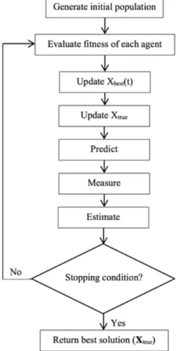
The simulated Kalman filter (SKF) [1, 11] algorithm is shown in Figure 1. The algorithm started with initialization of n agents, in which the positions of each agent are initialized randomly in the search space. The maximum number of iterations, tmax, is defined as the stopping condition for the algorithm. The initial value of error covariance estimate, 𝑃(0), the process noise value, 𝑄, and the measurement noise value, 𝑅, which are needed in Kalman filtering, are also determined during initialization stage. After that, each agent is subjected to fitness evaluation to generate initial solutions. The fitness values are checked and the agent having the best fitness value at every iteration, t, is recorded as Xbest(t). For function

minimization problem,

𝑿𝒃𝒆𝒔𝒕(𝑡) = min_1∈3,….,7𝑓𝑖𝑡1(𝑿(𝑡)) (1)

and for function maximization problem,

𝑿𝒃𝒆𝒔𝒕(𝑡) = max_1∈3,….,7𝑓𝑖𝑡1<𝑿(𝑡)= (2)

The best so far solution in SKF is named as Xtrue. The

Xtrue is updated only if the Xbest(t) is better (𝑿𝒃𝒆𝒔𝒕(𝑡) <

𝑿_{𝒕𝒓𝒖𝒆} for minimization problem, or 𝑿_{𝒃𝒆𝒔𝒕}(𝑡) > 𝑿𝒕𝒓𝒖𝒆

for maximization problem) than the Xtrue.

The subsequent computations are basically identical to the prediction, measurement and estimation procedures in Kalman filter. In the prediction stage, the following time-update equations are calculated: 𝑿_𝒊(𝑡|𝑡) = 𝑿_𝒊(𝑡) (3) 𝑃(𝑡|𝑡) = 𝑃(𝑡) + 𝑄 (4) where Xi(t) and Xi(t|t) are the previous state and predicted state, respectively, and P(t) and P(t|t) are previous error covariant estimate and predicted error covariant estimate, respectively. Note that the error

(3)

covariant estimate is influenced by the process noise,

Q.

Figure 1. Simulated Kalman filter (SKF) algorithm. The next step is measurement, which is a feedback to estimation process. Measurement is modelled such that its output may take any value from the predicted state estimate, 𝑿₁(𝑡|𝑡), to the true value, 𝑿_EFGH. Measurement, Zi(t), of each individual agent is simulated based on the following equation:

𝒁_𝒊(𝑡) = 𝑿𝒊(𝑡|𝑡) + sin(𝑟𝑎𝑛𝑑 × 2𝜋) × |𝑿𝒊(𝑡|𝑡) −

𝑿𝒕𝒓𝒖𝒆| (5)

The sin(𝑟𝑎𝑛𝑑 × 2𝜋) term provides the stochastic aspect of SKF algorithm and 𝑟𝑎𝑛𝑑 is a uniformly distributed random number in the range of [0,1].

The final step is the estimation. During this step, Kalman gain, 𝐾(𝑡), is computed as follows:

𝐾(𝑡) =_W(E|E)XYW(E|E) (6) Then, the estimation of next state, Xi(t+1), is computed based on Equation 7 and the error covariant

is updated based on Equation 8. Finally, the algorithm will continue the search process until the maximum number of iterations, tmax, is reached.

𝑿₁(𝑡 + 1) = 𝑿1(𝑡|𝑡) + 𝐾(𝑡) × (𝒁1(𝑡) − 𝑿1(𝑡|𝑡)) (7)

𝑃(𝑡 + 1) = <1 − 𝐾(𝑡)= × 𝑃(𝑡|𝑡) (8) Since the introduction of the SKF algorithm, fundamental studies [12-15] have been reported to understand the potentials of the SKF algorithm. Furthermore, fundamental modifications also been done to enhance the performance of the SKF [16-22], to enable the SKF to operate in discrete domains [23-28], and to solve multi-objective optimization problems [29]. The SKF has also been applied to solve engineering problems. For example, the SKF have employed as feature selector [30-33], algorithms in adaptive beamforming [34-37], routing algorithm in manufacturing process [38-40] and airport gate allocation [41], tuning algorithm in control engineering [42-45], and matching algorithm in image processing [46-48].

Opposition-based learning

The concept of Opposition-based learning (OBL) is to concurrently assess the current solutions and its opposite solutions in order to obtain a better approximation of the current candidate solutions. Figure 2 illustrate the opposite point which is determined in domain [a,b]. Let 𝑥 ∈ [𝑎, 𝑏] be a minimum and maximum values of variable in current population. The opposite number ox is determined as: 𝑜𝑥 = 𝑎 + 𝑏 − 𝑥 (9)

Figure 2. Opposite point defined in domain [a,b].

Current optimum opposition-based learning

In the original OBL concept, the agents and their opposite agents are asymmetric on the midpoint within the range of variables’ current interval. This opposite agents might possibly flee from the global optimum, which leads to decrease the contribution of opposite points. Therefore, opposition-based learning using the current optimum (COOBL) was proposed in [7] to address this drawback. So this approach is used to enhance the effectiveness of the SKF. The proposed algorithm is known as current optimum opposition-based simulated Kalman filter (COOBSKF).

The significant difference is the formation of opposite population in COOBSKF is depends on the

(4)

best agent so far which is identified by fitness calculation on particular objective function. The opposite population is generated using Equation 10.

𝑜𝑥1 = 2𝑥^_− 𝑥1 (10)

where 𝑥^_ is the best agent so far or current optimum

agent.

Enhancing SKF using current optimum

opposition-based learning

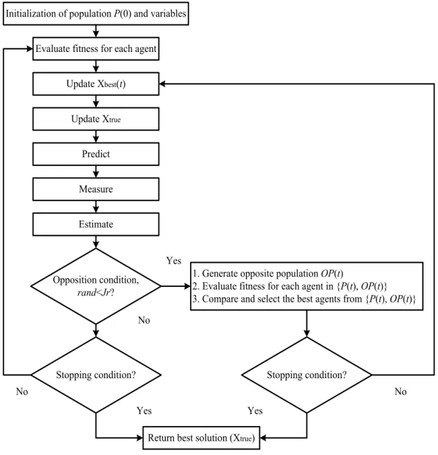
The original SKF is selected as a parent algorithm and the COOBL strategies are embedded in SKF to boost its performance. COOBL is employed at one stage of SKF which is after estimation process of SKF. This implementation generated opposite population which is potentially fitter compared to the current ones. Figure 3 shows the flowchart of the proposed algorithm.

Initially, COOBSKF generates randomly initial population or candidate solutions. The initial value of error covariance estimate, 𝑃(0), the process noise value, 𝑄, the measurement noise value, 𝑅, and jumping rate value, Jr, are also determined during initialization stage. Then, the fitness of agents in the population is calculated based on the objective function. Next, Xbest(t) and Xtrue are updated based on

SKF algorithm steps. The algorithm continues with prediction, measurement and estimation similar to SKF algorithm using Equation 3 to Equation 8.

After that, COOBL is applied to the current solution in order to check a potential solution on opposite side. This action is performed probabilistically influenced by a parameter known as the jumping rate, Jr ∈ [0,1]. Jr is a control parameter to form or ignore the formation of opposite population at specific iteration. The following jumping condition is considered:

Figure 3. Flowchart of COOBSKF algorithm. Evaluate fitness for each agent

Update Xbest(t) Update Xtrue Predict Measure Estimate Opposition condition, rand<Jr?

Initialization of population P(0) and variables

Stopping condition?

Return best solution (Xtrue)

1. Generate opposite population OP(t)

2. Evaluate fitness for each agent in {P(t), OP(t)} 3. Compare and select the best agents from {P(t), OP(t)}

Stopping condition? Yes Yes No No Yes No

(5)

if rand < Jr

then

apply COOBL else

check stopping condition else

where rand is a random number in the range of [0,1]. Within this stage, if opposition condition is met, the respective opposite population is formed according to Equation 10. Then, the best agents for next generation will be selected as follows:

𝑥₁(𝑡 + 1) = `𝑜𝑥1(𝑡), 𝑓𝑖𝑡 <𝑜𝑥1(𝑡)= < 𝑓𝑖𝑡 <𝑥1(𝑡)=

𝑥1(𝑡), 𝑓𝑖𝑡 (𝑜𝑥1(𝑡)) > 𝑓𝑖𝑡 (𝑥1(𝑡))

(11) Finally, the process of searching for optimum solution continued until the maximum number of function evaluation is reached.

Experimental and results

In order to make a fair comparison of the SKF and the proposed COOBSKF, we used a test suite of 30 standard benchmark functions and the same settings.

Benchmark functions

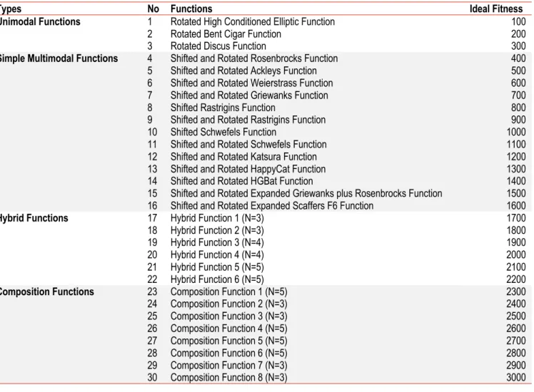
A comprehensive list of 30 benchmark global optimization functions (CEC 2014) [49] has been employed for performance verification of the proposed algorithms. The description of the benchmark functions and their global optimum (ideal fitness) are listed in Table 1. All the functions used in this experiment are minimization problem. It comes with 3 unimodal functions, 13 simple multimodal functions, 6 hybrid functions and 8 composition functions. The search space for all the test functions is between -100 to 100 for all dimensions.

Table 2. SKF parameters.

SKF Parameters Values

Initial error covariance estimate, P (0) 1000

Process noise, Q 0.5

Measurement noise, R 0.5

Table 3. Experimental parameters.

Experimental Parameters Values

Number of agent 100

Number of dimension 50

Number of run 50

Number of function evaluations 10000

Table 1. CEC 2014 benchmark functions.

Types No Functions Ideal Fitness

Unimodal Functions 1 Rotated High Conditioned Elliptic Function 100

2 Rotated Bent Cigar Function 200

3 Rotated Discus Function 300

Simple Multimodal Functions 4 Shifted and Rotated Rosenbrocks Function 400

5 Shifted and Rotated Ackleys Function 500

6 Shifted and Rotated Weierstrass Function 600

7 Shifted and Rotated Griewanks Function 700

8 Shifted Rastrigins Function 800

9 Shifted and Rotated Rastrigins Function 900

10 Shifted Schwefels Function 1000

11 Shifted and Rotated Schwefels Function 1100

12 Shifted and Rotated Katsura Function 1200

13 Shifted and Rotated HappyCat Function 1300

14 Shifted and Rotated HGBat Function 1400

15 Shifted and Rotated Expanded Griewanks plus Rosenbrocks Function 1500 16 Shifted and Rotated Expanded Scaffers F6 Function 1600

Hybrid Functions 17 Hybrid Function 1 (N=3) 1700

18 Hybrid Function 2 (N=3) 1800

Composition Functions 23 Composition Function 1 (N=5) 2300

24 Composition Function 2 (N=3) 2400 25 Composition Function 3 (N=3) 2500 26 Composition Function 4 (N=5) 2600 27 Composition Function 5 (N=5) 2700 28 Composition Function 6 (N=5) 2800 29 Composition Function 7 (N=3) 2900 30 Composition Function 8 (N=3) 3000

(6)

Settings for the experiments

In order to compare the performance of COOBSKF with the original SKF, all the experiments were executed in the same platform and subjected to the similar parameter settings in order to get a fair competition. Table 2 and Table 3 show the SKF parameters and experimental parameters respectively.

The stopping condition is defined to be the

maximum number of function evaluations for all

algorithms. Besides that, these experiments also

have been conducted to explore the effect of

jumping rate (

Jr

) upon the overall performance of

COOBSKF algorithm. The performance can vary

for different

Jr

values. To identify appropriate

Jr

value, the different numbers from 0 to 1 (0.1, 0.3

0.5, 0.7 and 0.9) was applied. Zero

Jr

means that

opposition-based technique is totally removed

from the algorithm. The

Jr

value is an important

control parameter in which, if optimally set, will

attain better results.

The performance of COOBSKF over SKF

This experiment investigates the performance of COOBSKF over the SKF. Based on Table 4, the

results obtained show that the proposed COOBSKF has a significant improvement.

According to Friedman Test, the average rankings of these algorithms are shown in Table 5. These algorithms can be sorted by average ranking into the following order: COOBSKF (Jr=0.9), COOBSKF (Jr=0.5), COOBSKF (Jr=0.7), COOBSKF (Jr=0.3), COOBSKF (Jr=0.1) and SKF. The best average ranking is obtained by the COOBSKF (Jr=0.9). The Friedman statistic for this experiment is 47.295. Since this value is greater than 11.070 (based on 5 degree of freedom at a 0.05 level of significance according to Chi-square table), hence, significant difference exists in term of performance among these algorithms.

Therefore, to compare the performance differences between these algorithms, the Friedman Post Hoc Test was performed. Post Hoc Test using Holm’s procedure is chosen to evaluate the significant difference between the algorithms’ performance [50]. Table 6 shows the resultant p-values when comparing between SKF and COOBSKF. Holm’s procedure rejects those hypotheses that have p-value lower than 0.005. The rejection of these hypotheses indicates a significant difference exists between the performances of the compared algorithms. The p-values below 0.005 are

Table 4. Mean value comparison of COOBSKF with SKF.

Function SKF COOBSKF

(Jr=0.1) COOBSKF (Jr=0.3) COOBSKF (Jr=0.5) COOBSKF (Jr=0.7) COOBSKF (Jr=0.9) 1 4702013.17 1076066.9455 1229553.6314 1295419.0349 1539599.2793 1709933.4488 2 24498691.66 3734.4152 4364.2133 5191.9996 5896.5624 5252.6651 3 18147.70 3576.0458 2508.6555 3106.0056 3433.6582 3283.6733 4 532.77 490.7681 509.5353 497.4695 521.1160 503.8873 5 520.01 520.0000 520.0000 520.0000 520.0000 520.0000 6 633.44 629.1087 627.1215 625.8455 625.6539 626.4995 7 700.25 700.0191 700.0172 700.0140 700.0141 700.0130 8 807.98 802.6068 801.9899 801.3332 801.6516 801.2735 9 1059.14 1054.8748 1053.5615 1051.9098 1054.7753 1058.2776 10 1335.18 1269.6576 1211.2699 1211.5394 1202.4715 1174.6086 11 6249.37 6058.5216 6089.7465 6154.4400 5909.7128 5964.2966 12 1200.24 1200.1665 1200.1602 1200.1510 1200.1523 1200.1509 13 1300.56 1300.5692 1300.5758 1300.5593 1300.5460 1300.5406 14 1400.30 1400.3079 1400.3219 1400.3350 1400.3479 1400.3294 15 1551.66 1523.9582 1520.5517 1520.1406 1518.5534 1519.0694 16 1619.13 1619.1377 1619.0205 1618.8370 1618.6569 1618.9107 17 908272.09 142202.2586 162138.3897 193156.7732 184132.1261 223642.6456 18 6941389.77 2889.1810 2900.4436 2943.6296 2805.0259 2928.3890 19 1950.22 1917.8190 1918.1752 1920.2604 1923.5501 1924.6712 20 34799.06 3952.7988 2760.8150 2919.4987 2723.6052 2574.2365 21 1186640.91 151359.6270 120710.0306 138331.9163 160142.6513 163087.1809 22 3429.11 3346.0273 3291.2296 3268.7018 3298.4063 3329.7652 23 2645.69 2644.0045 2644.0045 2644.0045 2644.0045 2644.0045 24 2667.25 2663.7930 2664.1926 2664.5113 2664.2735 2665.1893 25 2730.40 2725.1857 2719.1827 2716.7524 2718.2685 2717.4820 26 2766.39 2772.2931 2760.3367 2760.3725 2749.5381 2750.4254 27 3883.34 3764.6612 3763.2763 3760.4055 3742.2586 3703.4934 28 7223.37 6131.1664 5720.3915 5386.0278 5293.3785 5244.8513 29 5997.83 104245.4826 882355.6217 824794.4430 826387.6088 5448.3110 30 19753.29 16472.8260 17281.6365 16704.7432 17416.0645 17128.4940

(7)

shown in bold. According to the results, COOBSKF is significantly better than SKF.

Table 5. Average rankings of COOBSKF and SKF.

Algorithms Ranking COOBSKF (Jr=0.9) 1 COOBSKF (Jr=0.5) 2 COOBSKF (Jr=0.7) 3 COOBSKF (Jr=0.3) 4 COOBSKF (Jr=0.1) 5 SKF 6

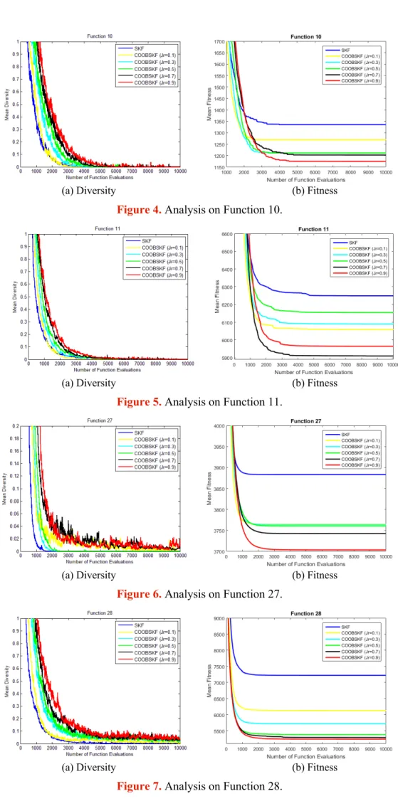
Figure 4 to Figure 7 show the diversity analysis of COOBSKF and its impact on algorithm’s performance for some CEC 2014 benchmark functions. Based on these figures, it shows that the higher Jr value is set, the higher diversity of population generated by COOBSKF. The high value of population diversity corresponds to good exploration and vice versa.

Table 6. Algorithms p-values table for α = 0.05.

Algorithms z p Holm SKF vs. COOBSKF (Jr=0.9) 5.7275 0.0000 0.0033 SKF vs. COOBSKF (Jr=0.5) 5.5205 0.0000 0.0036 SKF vs. COOBSKF (Jr=0.7) 5.4515 0.0000 0.0038 SKF vs. COOBSKF (Jr=0.3) 4.8305 0.0000 0.0042 SKF vs. COOBSKF (Jr=0.1) 4.1404 0.0000 0.0045 Based on those figures and statistical analysis performed previously, the higher diversity appears to be helpful to improve the search efficiency. This is due to the strength of current optimum opposition-based learning (COOBL) technique when generating the opposite agents. The formation of opposite agents is depended on the far. The best-agent-so-far is used as symmetry point between agents and their opposite agents, which increase the chance to locate the global optimum solution.

To conclude, the jumping rate is an important control parameter in which, if optimally set, can achieve even better results. Based on statistical analysis (considering all CEC2014 benchmark functions), the optimal Jr value for COOBSKF is 0.9.

The performance of COOBSKF over other

optimization algorithms

This experiment investigates the performance of COOBSKF in comparison with other optimization algorithms such as particle swarm optimization (PSO), grey wolf optimizer (GWO), genetic algorithm (GA), gravitational search algorithm (GSA) and black hole (BH). The experimental parameters used in this experiment are shown in Table 7. For COOBSKF, the

Jr value used is 0.9. For GSA, α is set to 20 and initial gravitational constant, G0 is set to 100. For PSO, cognitive coefficient, c1, and social coefficient, c2, are set to 2. The inertia factor is linearly decreased from 0.9 to 0.4. For GWO, components of a are linearly

decreased from 2 to 0. Lastly, for GA, the probabilities of selection and mutation are set to 0.5 and 0.2, respectively.

Table 7. Experimental parameters. Experimental Parameters Values

Population size 100

Number of dimensions 50

Number of runs 50

Number of function evaluations 10000

Jumping Rate, Jr 0.9

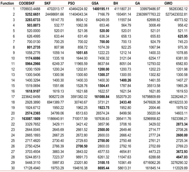
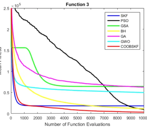
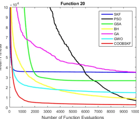
The results of each algorithm are presented in Table 8. In general, the COOBSKF and GSA show excellent performance on many test functions. According to the Friedman Test, the average rankings of these algorithms are shown in Table 9. These algorithms can be sorted by average ranking into the following order: COOBSKF, GSA, SKF, BH, PSO, GWO and GA. The best average ranking is obtained by the COOBSKF. The Friedman statistic for this experiment is 66.482. Since this value is greater than 12.592 (based on 6 degree of freedom at a 0.05 level of significance according to Chi-square table), significant difference exists in term of performance among these algorithms. Therefore, to compare the performance differences significantly between these algorithms, the Friedman Post Hoc Test was performed. Table 10 shows the resultant p-values when comparing between COOBSKF and the other optimization algorithms. Holm’s procedure rejects those hypotheses that have p-value lower than 0.0045. The rejection of these hypotheses indicates a significant difference exists between the performances of the compared algorithms. The p-values below 0.0045 are shown in bold. From the results, it can be seen that COOBSKF is significantly better than GA, GWO, PSO, BH, and SKF. The COOBSKF obtains the best result and the GSA has the second-best performance. Figure 8 to Figure 11 show the convergence curve for Function 3, Function 6, Function 20 and Function 27, respectively. Based on these figures, the COOBSKF has good convergence performance than the other compared algorithms.

Conclusion

This paper reports the first attempt to enhance the exploration capability of SKF by applying COOBL technique. In addition, jumping rate is also integrated in the proposed method. Once the jumping rate condition is met, the opposite solution is selected if the solution is better than the current one. The analysis confirmed that the proposed COOBSKF is superior to SKF and better than GA, GWO, PSO and BH. For future research, different OBL techniques shall be considered to enhance further the SKF.

(8)

(a) Diversity (b) Fitness

Figure 4. Analysis on Function 10.

(9)

Table 8. Mean value comparison of COOBSKF with other optimization algorithms.

Function COOBSKF SKF PSO GSA BH GA GWO

1 1709933.4488 4702013.17 43464224.92 1400195.11 4111807.31 339979486.97 56283362.12 2 5252.6651 24498691.66 11404043.34 7166.79 193491.14 23639977763.22 5273423032.81 3 3283.6733 18147.70 9934.12 64249.05 11557.54 62699.82 49773.52 4 503.8873 532.77 1062.06 653.46 564.79 3008.49 958.42 5 520.0000 520.01 521.06 520.00 520.01 521.01 521.11 6 626.4995 633.44 631.49 636.34 658.13 655.83 625.95 7 700.0130 700.25 700.02 700.00 700.13 924.79 745.23 8 801.2735 807.98 858.72 1074.39 922.25 1067.94 975.30 9 1058.2776 1059.14 1051.65 1222.23 1212.14 1400.33 1078.85 10 1174.6086 1335.18 1644.00 7456.32 3121.04 6254.17 6381.00 11 5964.2966 6249.37 11965.59 8637.64 8051.04 12793.02 6582.83 12 1200.1509 1200.24 1202.61 1200.00 1200.73 1202.23 1201.98 13 1300.5406 1300.56 1300.60 1300.37 1300.55 1302.82 1300.58 14 1400.3294 1400.30 1400.33 1400.30 1400.26 1461.55 1407.27 15 1519.0694 1551.66 1528.76 1504.41 1787.84 35513.58 1965.26 16 1618.9107 1619.13 1621.68 1622.57 1621.54 1621.85 1619.53 17 223642.6456 908272.09 3591382.02 161088.84 552079.20 16798809.69 3226248.21 18 2928.3890 6941389.77 30740.67 3731.21 2433.40 5476926.38 48192233.30 19 1924.6712 1950.22 1962.25 1923.75 1952.80 2004.46 1979.52 20 2574.2365 34799.06 6513.63 26574.24 8499.56 35020.04 14603.11 21 163087.1809 1186640.91 710017.59 187636.63 395411.76 5296958.82 1923398.21 22 3329.7652 3429.11 3421.42 3857.96 3708.16 3429.02 2873.34 23 2644.0045 2645.69 2661.52 2500.00 2649.46 2714.77 2708.26 24 2665.1893 2667.25 2672.80 2600.03 2666.42 2777.24 2600.00 25 2717.4820 2730.40 2729.83 2700.00 2750.48 2761.21 2725.34 26 2750.4254 2766.39 2700.50 2800.03 2792.16 2702.69 2769.23 27 3703.4934 3883.34 3843.02 4577.53 4654.81 4473.23 3672.93 28 5244.8513 7223.37 9891.73 6261.32 11047.63 6288.68 4647.03 29 5448.3110 5997.83 23201.80 3100.15 10361.49 6716062.26 3276290.32 30 17128.4940 19753.29 194616.38 8695.44 58613.31 161845.14 112029.89

Table 9. Average rankings of COOBSKF and others.

Algorithms Ranking COOBSKF 1 GSA 2 SKF 3 BH 4 PSO 5 GWO 6 GA 7

Table 10. Algorithms p-values table for α = 0.05.

Algorithms z p Holm COOBSKF vs. GA 7.7989 0.0000 0.0024 COOBSKF vs. GWO 4.8706 0.0000 0.0026 COOBSKF vs. PSO 4.4522 0.0000 0.0028 COOBSKF vs. BH 4.0638 0.0000 0.0031 COOBSKF vs. SKF 3.4960 0.0005 0.0036 COOBSKF vs. GSA 2.7191 0.0065 0.0045

(10)

(11)

(12)

Acknowledgement

The authors would like to thank the Ministry of Higher Education Malaysia and Universiti Malaysia Pahang (UMP) for awarding Fundamental Research Grant Scheme (FRGS) (RDU160105) to financially support this research.

References

[1] Z. Ibrahim, N. H. Abdul Aziz, N. A. Ab. Aziz, S. Razali, M. I. Shapiai, S. W. Nawawi and M. S. Mohamad, “A Kalman filter approach for solving unimodal optimization problems,”

ICIC Express Letters, vol. 9, no. 12, pp. 3415-3422, 2015. [2] H. R. Tizhoosh, “Opposition-based learning: a new scheme

for machine intelligence,” in Computational Intelligence for Modelling, Control and Automation and International Conference on Intelligent Agents, Web Technologies and Internet Commerce, 2005, pp. 695-701.

[3] M. Ventresca and H. R. Tizhoosh, “Improving the convergence of backpropagation by opposite transfer functions,” in International Joint Conference on Neural Networks, 2006, pp. 4777-4784.

[4] S. Rahnamayan, H. R. Tizhoosh and M. M. Salama, “Opposition-based differential evolution algorithms,” in

IEEE Congress on Evolutionary Computation, 2006, pp. 2010-2017.

[5] H. Wang, H. Li, Y. Liu, C. Li and S. Zeng, “Opposition-based particle swarm algorithm with Cauchy mutation,” in

IEEE Congress on Evolutionary Computation, 2007, pp. 4750-4756.

[6] A. R. Malisia, “Investigating the application of opposition-based ideas to ant algorithms,” M.S. thesis, Univ. of Waterloo, Canada, 2007.

[7] Q. Xu, L. Wang, B. M. He and N. Wang, “Modified opposition-based differential evolution for function optimization,” Journal of Computational Information Systems, vol. 7, no 5, pp. 1582-1591, 2011.

[8] R. Kennedy and J. Eberhart, “Particle swarm optimization,” in Proceedings of IEEE International Conference on Neural Networks IV, 1995, pp. 1942-1948.

[9] E. Rashedi, H. Nezamabadi-Pour and S. Saryazdi, “GSA: a gravitational search algorithm,” Information Sciences, vol. 179, no. 13, pp. 2232-2248, 2009.

[10] S. Rahnamayan, H. R. Tizhoosh and M. M. Salama, “Opposition-based differential evolution,” IEEE Transactions on Evolutionary computation, vol. 12, no. 1, pp. 64-79, 2008.

[11] Z. Ibrahim, N. H. Abdul Aziz, N. A. Ab. Aziz, R. Razali and M. S. Mohamad, “Simulated Kalman filter: a novel estimation-based metaheuristic optimization algorithm,”

Advanced Science Letters, vol. 22, no. 10, pp. 2941-2946, 2016.

[12] N. H. Abdul Aziz, Z. Ibrahim, S. Razali, T. A. Bakare and N. A. Ab. Aziz, “How important the error covariance in simulated Kalman filter?,” in National Conference for Postgraduate Research, 2016, pp. 315-320.

[13] N. H. Abdul Aziz, N. A. Ab. Aziz, M. F. Mat Jusof, S. Razali, Z. Ibrahim, A. Adam and M. I. Shapiai, “An analysis on the number of agents towards the performance of the simulated Kalman filter optimizer,” in 8th International Conference on Intelligent Systems, Modelling and Simulation, 2018, pp. 16-21.

[14] N. H. Abdul Aziz, Z. Ibrahim, N. A. Ab. Aziz and S. Razali, “Parameter-less simulated Kalman filter,” International

3, pp. 129-137, 2017.

[15] N. H. Noordin, Z. Ibrahim, M. H. J. Xie, R. Samad and N. Hasan, “FPGA implementation of simulated Kalman filter optimization algorithm,” Journal of Telecommunication, Electronic and Computer Engineering, vol. 10, no. 1-3, pp. 21-24, 2018.

[16] B. Muhammad, Z. Ibrahim, K. H. Ghazali, K. Z. Mohd Azmi, N. A. Ab Aziz, N. H. Abd Aziz and M. S. Mohamad, “A new hybrid simulated Kalman filter and particle swarm optimization for continuous numerical optimization problems,” ARPN Journal of Engineering and Applied Sciences, vol. 10, no. 22, pp. 17171-17176, 2015.

[17] Z. Ibrahim, K. Z. Mohd Azmi, N. A. Ab. Aziz, N. H. Abdul Aziz, B. Muhammad, M. F. Mat Jusof and M. I. Shapiai, “An oppositional learning prediction operator for simulated Kalman filter,” in 3rd International Conference on Computational Intelligence and Applications, 2018, pp. 139-143.

[18] N. H. Abdul Aziz, Z. Ibrahim, N. A. Ab Aziz, M. S. Mohamad and J. Watada, “Single-solution simulated Kalman filter algorithm for global optimisation problems,”

Sadhana, vol. 43, no. 7, article 103, 2018.

[19] N. A. Ab. Aziz, Z. Ibrahim, N. H. Abdul Aziz and T. Ab. Rahman, “Asynchronous simulated Kalman filter optimization algorithm,” International Journal of Engineering and Technology(UAE), vol. 7, no. 4.27, pp. 44-49, 2018.

[20] B. Muhammad, Z. Ibrahim, K. Z. Mohd Azmi, K. H. Abas, N. A. Ab Aziz, N. H. Abd Aziz and M. S. Mohamad, “Performance evaluation of hybrid SKF algorithms: hybrid SKF-PSO and hybrid SKF-GSA,” in National Conference for Postgraduate Research, 2016, pp. 865-874.

[21] B. Muhammad, Z. Ibrahim, K. Z. Mohd Azmi, K. H. Abas, N. A. Ab Aziz, N. H. Abd Aziz and M. S. Mohamad, “Four different methods to hybrid simulated Kalman filter (SKF) with particle swarm optimization (PSO),” in National Conference for Postgraduate Research, 2016, pp. 843-853. [22] B. Muhammad, Z. Ibrahim, K. Z. Mohd Azmi, K. H. Abas,

N. A. Ab Aziz, N. H. Abd Aziz and M. S. Mohamad, “Four different methods to hybrid simulated Kalman filter (SKF) with gravitational search algorithm (GSA),” in National Conference for Postgraduate Research, 2016, pp. 854-864. [23] Z. Md Yusof, I. Ibrahim, Z. Ibrahim, K. H. Abas, N. A. Ab

Aziz, N. H. Abd Aziz and M. S. Mohamad, “Local optimum distance evaluated simulated Kalman filter for combinatorial optimization problems,” in National Conference for Postgraduate Research, 2016, pp. 892-901.

[24] Z. Md Yusof, I. Ibrahim, Z. Ibrahim, K. H. Abas, S. Sudin, N. A. Ab Aziz, N. H. Abd Aziz and M. S. Mohamad, “Three approaches to solve combinatorial optimization problems using simulated Kalman filter,” in National Conference for Postgraduate Research, 2016, pp. 951-960.

[25] Z. Md Yusof, I. Ibrahim, S. N. Satiman, Z. Ibrahim, N. H. Abd Aziz and N. A. Ab Aziz, “BSKF: binary simulated Kalman filter,” in Third International Conference on Artificial Intelligence, Modelling and Simulation, 2015, pp. 77-81.

[26] Z. Md Yusof, Z. Ibrahim, I. Ibrahim, K. Z. Mohd Azmi, N. A. Ab Aziz, N. H. Abd Aziz and M. S. Mohamad, “Angle modulated simulated Kalman filter algorithm for combinatorial optimization problems,” ARPN Journal of Engineering and Applied Sciences, vol. 11, no. 7, pp. 4854-4859, 2016.

[27] Z. Md Yusof, Z. Ibrahim, I. Ibrahim, K. Z. Mohd Azmi, N. A. Ab. Aziz, N. H. Abd Aziz and M. S. Mohamad, “Distance evaluated simulated Kalman filter for combinatorial

(13)

optimization problems,” ARPN Journal of Engineering and Applied Sciences, vol. 11, no. 7, pp. 4904-4910, 2016. [28] Z. Md Yusof, Z. Ibrahim, A. Adam, K. Z. Mohd Azmi, T. Ab

Rahman, B. Muhammad, N. A. Ab Aziz, N. H. Abd Aziz, N. Mokhtar, M. I. Shapiai and M. S. Muhammad, “Distance evaluated simulated Kalman filter with state encoding for combinatorial optimization problems,” International Journal of Engineering and Technology(UAE), vol. 7, no. 4.27, pp. 22-29, 2018.

[29] A. Azwan, A. Razak, M. F. M. Jusof, A. N. K. Nasir and M. A. Ahmad, “A multiobjective simulated Kalman filter optimization algorithm,” in 4th IEEE International Conference on Applied System Innovation, 2018, pp. 23-26. [30] A. Adam, Z. Ibrahim, N. Mokhtar, M. I. Shapiai, M. Mubin and I. Saad, “Feature selection using angle modulated simulated Kalman filter for peak classification of EEG signals,” SpringerPlus, vol. 5, no. 1580, 2016.

[31] B. Muhammad, M. F. Mat Jusof, A. Adam, Z. Md Yusof, K. Z. Mohd Azmi, N. H. Abdul Aziz, Z. Ibrahim, M. I. Shapiai and N. Mokhtar, “Feature selection using binary simulated Kalman filter for peak classification of EEG Signals,” in 8th International Conference on Intelligent Systems, Modelling and Simulation, 2018, pp. 1-6.

[32] A. Adam and B. Muhammad, “Distance evaluated simulated kalman filter algorithm for peak classification of EEG signals,” International Journal of Simulation: Systems, Science and Technology, vol. 19, no. 5, pp. 6.1-6.7, 2018. [33] N. Ahmad Zamri, T. Bhuvanewari, N. A. Ab. Aziz and N. H.

Abdul Aziz, “Feature selection using simulated Kalman filter (SKF) for prediction of body fat percentage,” in

International Conference on Mathematics and Statistics, 2018, pp. 23-27.

[34] K. Lazarus, N. H. Noordin, Z. Ibrahim and K. H. Abas, “Adaptive beamforming algorithm based on simulated Kalman filter,” in Asia Multi Conference on Modelling and Simulation, 2016, pp. 19-23.

[35] K. Lazarus, N. H. Noordin, K. Z. Mohd Azmi, N. H. Abdul Aziz and Z. Ibrahim, “Adaptive beamforming algorithm based on generalized opposition-based simulated Kalman filter,” in National Conference for Postgraduate Research, 2016, pp. 1-9.

[36] K. Lazarus, N. H. Noordin, M. F. Mat Jusof, Z. Ibrahim and K. H. Abas, “Adaptive beamforming algorithm based on simulated Kalman filter,” International Journal of Simulation: Systems, Science and Technology, vol. 18, no. 4, pp. 10.1-10.5, 2017.

[37] K. Lazarus, N. H. Noordin, Z. Ibrahim, M. F. Mat Jusof, A. A. Mohd Faudzi, N. Subari and K. Z. Mohd Azmi, “An opposition-based simulated Kalman filter algorithm for adaptive beamforming,” in IEEE International Conference on Applied System Innovation, 2017, pp. 91-94.

[38] N. H. Abdul Aziz, N. A. Ab Aziz, Z. Ibrahim, S. Razali, K. H. Abas and M. S. Mohamad, “A Kalman filter approach to PCB drill path optimization problem,” in IEEE Conference on Systems, Process and Control, 2016, pp. 33-36.

[39] A. Mustafa, Z. M. Yusof, A. Adam, B. Muhammad and Z. Ibrahim, “Solving assembly sequence planning using angle modulated simulated Kalman filter,” IOP Conference Series: Materials Science and Engineering, vol. 319, no. 1, Article number 012044, 2018.

[40] N. H. Abdul Aziz, Z. Ibrahim, N. A. Ab. Aziz, Z. Md Yusof and M. S. Mohamad, “Single-solution simulated Kalman filter algorithm for routing in printed circuit board drilling process,” Intelligent Manufacturing and Mechatronics, pp. 649-655, 2018.

[41] K. Z. Mohd Azmi, Z. Md Yusof, S. N. Satiman, B. Muhammad, S. Razali, Z. Ibrahim, N. A. Ab. Aziz and N. H.

Abd Aziz, “Solving airport gate allocation problem using angle modulated simulated Kalman filter,” in National Conference for Postgraduate Research, 2016, pp. 875-885. [42] M. F. M. Jusof, A. N. K. Nasir, M. A. Ahmad and Z. Ibrahim,

“An exponential based simulated Kalman filter algorithm for data-driven PID tuning in liquid slosh controller,” in 4th IEEE International Conference on Applied System Innovation, 2018, pp. 984-987.

[43] B. Muhammad, D. Pebrianti, N. A. Ghani, N. H. Abdul Aziz, N. A. Ab. Aziz, M. S. Mohamad, M. I. Shapiai and Z. Ibrahim,” An application of simulated Kalman filter optimization algorithm for parameter tuning in proportional-integral-derivative controllers for automatic voltage regulator system,” in SICE International Symposium on Control Systems, 2018, pp. 113-120.

[44] B. Muhammad, K. Z. Mohd Azmi, Z. Ibrahim, A. A. Mohd Faudzi and D. Pebrianti, “Simultaneous computation of model order and parameter estimation for system identification based on opposition-based simulated Kalman filter,” in SICE International Symposium on Control Systems, 2018, pp. 105-112.

[45] K. Z. Mohd Azmi, Z. Ibrahim, D. Pebrianti and M. S. Mohamad, “Simultaneous computation of model order and parameter estimation for ARX model based on single and multi swarm simulated Kalman filter,” Journal of Telecommunication, Electronic, and Computer Engineering, vol. 9, no. 1-3, pp. 151-155, 2017.

[46] N. Q. Ann, D. Pebrianti, Z. Ibrahim, M. F. Mat Jusof, L. Bayuaji and N. R. H. Abdullah, “Illumination-invariant image matching based on simulated Kalman filter (SKF) algorithm,” Journal of Telecommunication, Electronic and Computer Engineering, vol. 10, no. 1-3, pp. 31-36, 2018. [47] N. Q. Ann, D. Pebrianti, Z. Ibrahim, L. Bayuaji and M. F.

Mat Jusoh, “Image template matching based on simulated Kalman filter (SKF) algorithm,” Journal of Telecommunication, Electronic and Computer Engineering, vol. 10, no. 2-7, pp. 37-41, 2018.

[48] N. Q. Ann, D. Pebrianti, L. Bayuaji, M. R. Daud, R. Samad, Z. Ibrahim, R. Hamid and M. Syafrullah, “SKF-based image template matching for distance measurement by using stereo vision,” Intelligent Manufacturing & Mechatronics, pp. 439-447, 2018.

[49] Liang, J. J., Qu, B. Y., & Suganthan, P. N., “Problem definitions and evaluation criteria for the CEC 2014 special session and competition on single objective real-parameter numerical optimization,” Computational Intelligence Laboratory, Zhengzhou University, Zhengzhou, China, Tech. Rep. 201311 and Nanyang Technological University, Singapore, 2013.

[50] J. Derrac, S. García, D. Molina and F. Herrera, “A practical tutorial on the use of nonparametric statistical tests as a methodology for comparing evolutionary and swarm intelligence algorithms,” Swarm and Evolutionary Computation, vol. 1, no. 1, pp. 3-18, 2011.