Tax Policy and Employment: How Does the Swedish System Fare?

Uppsala Center for Fiscal Studies

Department of Economics

Working Paper 2011:2

Tax Policy and Employment: How Does

the Swedish System Fare?

Uppsala Center for Fiscal Studies Working paper 2011:2 Department of Economics February 2011

Uppsala University P.O. Box 513

SE-751 20 Uppsala Sweden

Fax: +46 18 471 14 78

T

P

E

: H

d

s

s

F

?

Papers in the Working Paper Series are published on internet in PDF formats. Download from http://ucfs.nek.uu.se/

Tax Policy and Employment: How Does the Swedish System Fare? by Jukka Pirttilä and Håkan Selin February 1, 2011

Abstract: This paper reviews the literature on optimal taxation of labour income and the empirical work on labour supply and the elasticity of taxable income in Sweden. It also presents an overview of Swedish taxation of labour income, offers calculations on the development in effective marginal tax rates and participation tax rates, and estimates, using the difference-in-differences method, the impact of tax incentives on employment rates of elderly workers. After this background, we ponder possibilities for reforming the Swedish tax system to improve its labour market impacts. We suggest better targeting the earned income tax credit at families and low-income workers, lowering the top marginal tax rates, and maintaining the tax incentives for older workers.

Key words: Optimal taxation, labour income taxation, labour supply, taxable income, Swedish tax system.

JEL codes: H21; H24; J22.

       

This paper was originally published in Swedish as "Skattepolitik och sysselsättning. Hur väl fungerar det svenska systemet?", bilaga 12 till Långtidsutredningen 2011, SOU 2011:2, Välfärdsstaten i arbete. Inkomsttrygghet och omfördelning med incitament till arbete. We are grateful to Mårten Hultin of the Swedish Ministry of Finance for help with the micro-simulations, to Lennart Flood and John Hassler, seminar participants and the editors for useful comments on an earlier draft.



University of Tampere and the Labour Institute for Economic Research, Helsinki. Department of Economics and Accounting, FI-33014 University of Tampere, Finland. Email: <jukka.pirttila@uta.fi>



Uppsala Center for Fiscal Studies at the Department of Economics, Uppsala University, P.O. Box 513, SE-751 20 Uppsala, Sweden, Email: <hakan.selin@nek.uu.se> 

1. Introduction

One of the most heavily debated topics in economics is the employment effects of taxation. Some macroeconomists argue that virtually all employment differences between countries are due to differences in the tax burden, whereas most economists specialising in labour and public economics hold the view that taxes matter somewhat; for some groups of workers they might matter more, whereas others seem to work regardless of the level of income or other taxation.

This article offers a selected review of both the theoretical and empirical economic research on taxation and employment that we think is most relevant for the current Swedish system. This review focuses on the microeconomic part of research, drawing on both applied theory and microeconometric evidence (i.e. statistical analysis using data on individuals, not countries), although we briefly comment on the relations between macro and micro work in Section 4 below.1 The purpose of our report is to discuss the Swedish system for the taxation of labour incomes in the light of the most recent theoretical and empirical findings on the intersection of labour and public economics.

Before starting the actual review, it might be useful to briefly describe the basic problem at hand: When setting taxes, the government typically wants to both raise revenues in an efficient manner (without distorting the economy too drastically or changing too much the way people work and save and the way firms invest) and to achieve a socially acceptable distribution of the tax burden and after-tax income. Taxation is also used to achieve other goals; for example, corrective taxes are imposed on externality-generating activities to equate private and marginal social costs, but these taxes are not the subject matter of this survey. The efficiency and equity objectives of taxation are to some extent conflicting objectives. If the government wants to achieve a very evenly distributed disposable income, it needs to rely on heavily progressive taxation and offer a comprehensive social safety net. However, such a policy reduces people’s incentives to work and save, as well as the firms’ incentives to invest, and therefore redistribution typically also diminishes the overall size of the economy, i.e. some efficiency losses are inevitable. Note that this is not a universal truth; one can imagine policies that are desirable as regards both efficiency and equity: To some extent, the social safety net can serve as one example if it also facilitates efficiency-increasing risk taking among the population. However, as a general rule, the trade off exists and the optimal choice

       1

This paper concentrates on the relation between employment and taxation. A recent impressive study by Sørensen (2010) offers a general analysis of the Swedish tax system – including analysis of international competitiveness and capital income taxation. On the other hand, it is somewhat less focused on employment effects. Many of the conclusions in Sørensen (2010) and our work are very similar, as we will discuss below.

depends on societal preferences. The more the government and the population value redistribution, the more they are willing to tolerate distortions to the economy.

A simple example, in which taxation affects individual decisions, is labour supply. If the marginal tax on labour income is raised, this reduces the take-home pay from work on the margin. This makes leisure relatively more attractive, and reduces the hours of work (economists call this a substitution effect). The greater is this effect, the more a given level of taxation distorts the economy. On the other hand, a higher level of taxation reduces people’s disposable income. If leisure is a good that people want to enjoy more when their income increases, making people poorer by increasing taxes also has an additional channel of influence that tends to increase labour supply (this is called ‘an income effect’). While the two effects point in opposite directions, the substitution effect typically dominates and therefore higher marginal taxes typically reduce labour supply.2 Hence, higher tax rates to fund more public expenditure or more progression to redistribute income typically entail some efficiency losses. How large these losses are, and to what extent the employment effects vary across different tax instruments or within the tax system, is the essence of what we will review in this report.

The next section of this report offers a brief description of the aspects of the Swedish tax system that are most relevant for employment. Particular emphasis will be put on incentives created by the tax and the transfer system to take paid work as opposed to unemployment or sickness leave. Section 3 reviews the theoretical literature on designing a good tax system based on lessons in what economists call ‘optimal tax theory’. Here, we draw heavily on recent material in the Mirrlees Review3, a large-scale overview of tax theory and practice by the world’s leading tax economists and lawyers, initiated by the Institute for Fiscal Studies in the UK. Section 4 turns to the empirical evidence on the connections between taxation and employment, using both international material and evidence from Sweden. Section 5 summarises our findings and discusses reform options to enhance the design of the Swedish tax system from the employment perspective.

       2

Although at high income levels, the income effect may be stronger, in which case a tax increase would actually increase labour supply for a subset of population.

3

2. The Swedish tax system

2.1 General features and recent reforms

Sweden is a high tax country by any standards. In 2008 the total revenue of the general government sector amounted to 53 % of GDP, whereas total public expenditures were 50.6 % of GDP. There are several ways to classify taxes. One is to distinguish between taxes on labour, taxes on capital and taxes on consumption and input goods. Table 2.1 reports the

collected revenues for each category in 2007. Table 2.1 shows that 59 % of the taxes

collected relate to labour income. From the decomposition of labour income taxes in Table 2.2 we recognize that the bulk of the tax revenues relating to labour income comes from local income tax (479 billion in 2007) and social security contributions (473 billion in 2007).

Table 2.1. Total taxes in 2007

SEK, billion % of total taxes % of GDP Taxes on labour 874 59% 28.5 % Taxes on capital 208 14% 6.8%

Taxes on consumption and input goods 402 27 % 13.1 %

Total taxes 1484 100% 48.4%

Source: Taxes in Sweden 2009 (Table 4).

In this report we analyse the optimal design of the labour income taxation and how taxes affect employment. The main emphasis will be on labour income taxation at the personal level and the supply side of the economy. Thus, we will mainly concentrate on how features of the personal income tax system affect individual behaviour. We will also discuss some issues in payroll taxation. However, from the viewpoint of economic theory there are no sharp dividing lines between ‘taxes on labour income’ and other taxes. First, standard economic textbooks teach that the statutory incidence of the tax does not say anything about the economic incidence of the tax. In other words, the agent who formally pays the tax does not necessarily bear the burden of the tax. Second, in some applications the implications of levying a consumption tax are analytically similar to levying an income tax. In a model where the individual disposes of all her income, and hence there is no saving, a proportional income tax of 50 % is equivalent to taxing consumption at a rate of 100%, if the tax on consumption is defined as a mark-up on the consumer price.

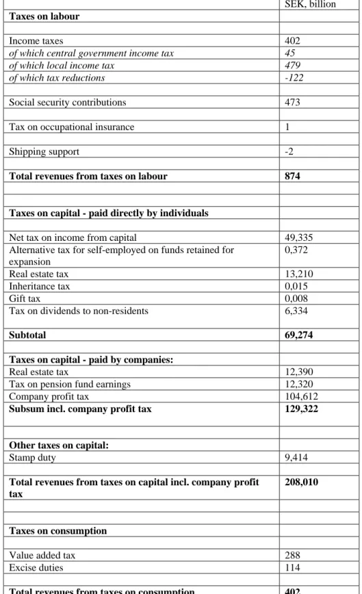
Table 2.2 Decomposition of tax revenues 2007

SEK, billion

Taxes on labour

Income taxes 402

of which central government income tax 45

of which local income tax 479

of which tax reductions -122

Social security contributions 473

Tax on occupational insurance 1

Shipping support -2

Total revenues from taxes on labour 874

Taxes on capital - paid directly by individuals

Net tax on income from capital 49,335

Alternative tax for self-employed on funds retained for expansion

0,372

Real estate tax 13,210

Inheritance tax 0,015

Gift tax 0,008

Tax on dividends to non-residents 6,334

Subtotal 69,274

Taxes on capital - paid by companies:

Real estate tax 12,390

Tax on pension fund earnings 12,320

Company profit tax 104,612

Subsum incl. company profit tax 129,322

Other taxes on capital:

Stamp duty 9,414

Total revenues from taxes on capital incl. company profit tax

208,010

Taxes on consumption

Value added tax 288

Excise duties 114

Total revenues from taxes on consumption 402

Source. Taxes in Sweden 2009, Table 14, Source: Taxes in Sweden 2009, Table 5, Source. Skattestatistisk årsbok 2009, table 5.1.

A centre-right wing coalition came into power in 2006. This change in power had quite a profound impact on the taxation of labour incomes. One of the stated purposes of the government’s tax policy was to

“…contribute to an increase of the permanent level of employment (the number of hours worked) via an increase in labour force participation, increase in work hours among those who are in the labour force and increase in education and competence among those who work.”4

The introduction of the so-called ‘jobbskatteavdraget’, the earned income tax credit (EITC) stands out as the single most important tax reform.5 However, changes have also been made in other areas of taxation with direct or indirect impact on work incentives. Some of the most important implemented tax cuts since the tax year of 2007 are

 An earned income tax credit was introduced in four steps 2007-2010.

 The tax burden on elderly workers was reduced both through targeted pay roll

tax reductions and a considerably more generous earned income tax credit for those aged 65 and above (2007).

 Payroll tax reductions were targeted towards young workers aged below 26

(2009).

 A tax reduction for household services was introduced (2007) and a tax

reduction for building, rebuilding and maintenance services (late 2008) was introduced.

 The property tax on owner-occupied housing was abolished and replaced by a

charge that may not exceed SEK 6000. (2008).

 The wealth tax was abolished (2007).

 The tax on corporate profits was lowered from 28 % to 26.3 % of profits (2009).

 The tax treatment of closely held corporations became more favorable

(2007-2008).

To a large extent the EITC has been financed by reforms in the social insurance system. Most prominently, changes have been made to the unemployment insurance system and the sickness insurance system.6

       4

Prop. 2008/09:1, p.135. Our translation. 5

In what follows we use the term ‘earned income tax credit (EITC)’ as a translation of ‘skattereduktion för arbetsinkomster’ which is often called ‘jobbskatteavdraget’ in the Swedish debate. EITC is the name of the U.S. in-work subsidy which has been in place since the 1970’s. One should keep in mind that there are several important differences between the Swedish and the U.S. earned income tax credits

6

2.2. The Swedish income tax system

The basic structure of the Swedish statutory income tax system, which to a large extent is a result of the comprehensive 1991 reform, is simple. A proportional local tax rate applies to all earned income and taxable transfers. The mean local income tax rate in 2010 is 31.56 %, with a minimum rate of 28.89 (Vellinge), and a maximum rate of 34.17 (Ragunda). For total labour incomes above a certain threshold, (SEK 384,200 in 2010), the taxpayer also has to pay a central government income tax. The central government income tax schedule consists of two brackets; the marginal tax rates in each bracket are 20% and 25% respectively. Thus, when only considering the personal income tax the top marginal tax rate on earned income is 56.56 % in 2010. Capital income is taxed separately from total labour income according to a proportional tax rate of 30 %.

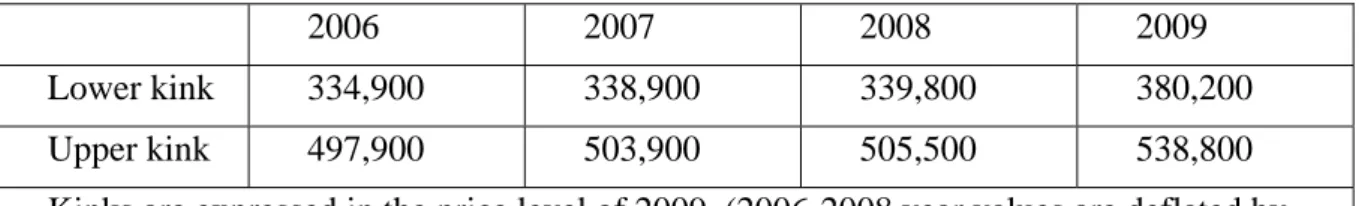
In 2007, 20 % of the population aged over 20 were liable to the central government income tax. Six per cent of the population faced the top marginal tax rate. The thresholds for the central government income tax increased in real terms during the last couple of years (Table 2.3). In particular, the kink points in central government taxation were increased in 2009.

Table 2.3. The upper and lower kink points of the central government tax schedule 2006-2009, SEK.

2006 2007 2008 2009

Lower kink 334,900 338,900 339,800 380,200

Upper kink 497,900 503,900 505,500 538,800

Kinks are expressed in the price level of 2009. (2006-2008 year values are deflated by the CPI).

Before computing the individual’s tax liability, a basic deduction is made mechanically by the tax authorities against the individual’s assessed total labour income (the sum of earned income and social transfers). Since 1991 the basic deduction has been phased in at lower income levels and phased out at higher income levels with consequences for the marginal tax rate facing the individual in these income intervals. Figure 2.1 shows the statutory tax schedule on individuals in 2010. The basic deduction is phased in between SEK 42,000 and SEK 115,300 and phased out between SEK 131,000 to SEK 334,100 in 2010.

2.2. The earned income tax credit

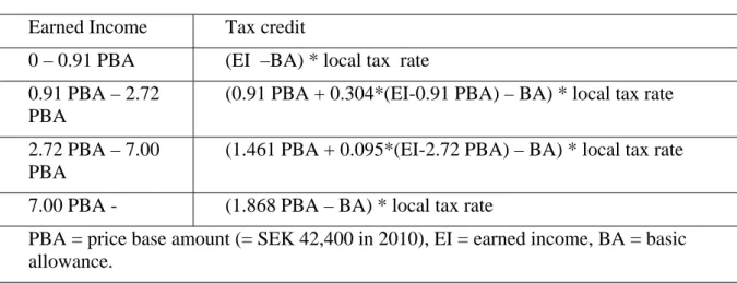
A Swedish earned income tax credit, which applies solely to earned income – and not to taxable transfers7 -- was introduced in 2007. In the 2007 government bill the budget cost of this tax cut (‘the first step’) was estimated to be around SEK 40 billion. The EITC reform marks a break with the longstanding Swedish tradition of taxing several types of social transfers together with earned income. The technical design of the EITC is complicated. This is partly due to the pre-existing basic allowance. The size of the EITC in 2010 is calculated in accordance with Table 2.4. The EITC lowers marginal tax rates up to a level of earned income of SEK 334,000. However, in contrast to what is standard in other countries that have implemented in-work tax credits the Swedish EITC is not phased out.

Table 2.4. Formula for the earned income tax credit in 2010

Earned Income Tax credit

0 – 0.91 PBA (EI –BA) * local tax rate

0.91 PBA – 2.72 PBA

(0.91 PBA + 0.304*(EI-0.91 PBA) – BA) * local tax rate 2.72 PBA – 7.00

PBA

(1.461 PBA + 0.095*(EI-2.72 PBA) – BA) * local tax rate

7.00 PBA - (1.868 PBA – BA) * local tax rate

PBA = price base amount (= SEK 42,400 in 2010), EI = earned income, BA = basic allowance.

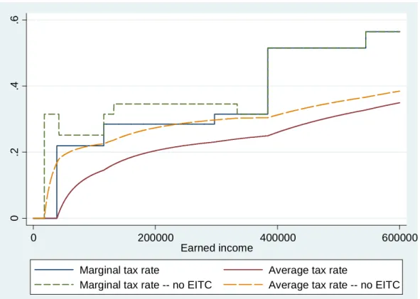
Figure 2.1 shows the marginal tax rate and average tax rate as a function of earned income, with and without the EITC in 2010 under the assumption that all reported income is earned income (not taxable transfers). In one sense, the EITC simplified the marginal tax schedule as

the number of brackets decreased from 8 to 6.8 A large number of taxpayers with middle

range incomes receive a marginal tax rate cut of approximately 6 percentage points. The marginal tax rates of those earning above SEK 334,000 are not affected by the EITC. We can also infer that taxpayers with very low incomes received dramatic cuts in both the average tax

       7

This is not completely true since the EITC also depends on the basic allowance, which is also a function of taxable transfers.

8

Note that this is on the assumption that the individual receives no taxable transfers. Since the basic deduction, but not the EITC, is a function of taxable transfers, the kink points in general depend on the amount of taxable transfers. This makes the tax code non-salient from the perspective of the taxpayers.

rate and marginal tax rate. For higher incomes the reduction in average tax rates is more modest. 0 .2 .4 .6 0 200000 400000 600000 Earned income

Marginal tax rate Average tax rate

Marginal tax rate -- no EITC Average tax rate -- no EITC

Figure 2.1. The marginal tax rate as a function of earned income (under the assumption that the individual receives no taxable transfers) in 2010. The tax schedule includes basic allowance, earned income tax credit and central government income tax.

The abovementioned rules apply to workers aged 65 or below. Elderly workers who earn wage income or self-employment income are subject to more generous rules. In 2007 and 2008 the EITC formula for elderly workers was quite similar to the formula for prime-aged workers, with the exception that elderly workers benefited from a more generous tax credit at a given level of earned income, see Appendix 4. In 2009 the EITC schedule for elderly workers was simplified so that it is no longer a function of either the local tax rate or the basic allowance – it is only a function of the amount of earned income.

2.3 Payroll taxes

The statutory payroll tax (social security contributions) in Sweden has been stable around 32-33 % of the gross wage since the mid 1990’s. On top of that, employers pay contributions to collectively agreed social benefit systems. One should keep in mind, though, that the social security contributions also entitle the employee to a number of social benefits. However, to a

large extent there is no direct link between the amount paid and the level of pension and benefits collected. Wage income exceeding 7.5 price base amounts does in general not generate any benefits. The tax component of the social security contributions has often been estimated to be around 60 % (The Swedish Tax Agency 2010, p. 11).

From July 1, 2007, the payroll tax rate was lowered to 22.71 % of the wage bill for individuals who had not turned 25 before January 1. From 1 January 2009 employers who have workers aged below 26 before 1 January only have to pay a social security contribution rate of 15.74 % for these employees. These reforms were motivated by high youth unemployment rates and demographic trends.

The government has also targeted payroll tax cuts at elderly workers. For employees born prior to 1938 the employer does not need to pay any statutory social security contributions. These workers are not eligible for the new public pension system. For those born after 1938 but who are 65 and older, the employer pays a social security contribution of 10.21 %, see Appendix 4 for details.

Related programs currently in place in Sweden reducing wage costs for certain groups of workers are “nystartsjobben”, “nyfriskjobben” and “instegsjobben”. “Nystartsjobben” implies a wage subsidy for the long-term unemployed, “Nyfriskjobben” is a subsidy to individuals who have been on long-term sick-leave. “Instegsjobben”, finally, is a wage subsidy targeted at newly arrived immigrants.

2.4. Consumption taxes

Consumption taxes can be divided into value added taxes (VAT) and excise duties. The general VAT rate is 25 %. Food, hotel accommodation and camping are taxed at a rate of 12%. Newspapers, books, magazines, cultural and sports events and passenger transports are taxed at 6 %. For a typical household the effective VAT rate is around 21 %.9 The bulk of excise duties is levied on energy and environmental taxes.

2.5. Tax reduction for household services

A tax reduction for household services was introduced on 1 July, 2007. The taxpayer receives a tax credit of 50 % of the cost of the household service. The tax reduction applies to services conducted close to the house or apartment where the taxpayer lives. These services include

       9

cleaning services, cooking, grasscutting and childcare. Almost 99,000 Swedish taxpayers applied for this tax reduction for the tax year 2008, see Section 5.3 for a further discussion.

A tax reduction for building, rebuilding and maintenance services, primarily for real estate, (ROT-avdraget) was reintroduced for purchases of this type of services from December 8, 2008 and onwards. This tax reduction has occasionally been in place earlier and has been motivated as a stimulus programme to the building industry. The tax reduction is again 50 % of the labour cost. The sum of these tax reductions (RUT + ROT) must not exceed SEK 50,000.

2.6. Microsimulation

In the previous sections we made the observation that the introduction of the EITC considerably lowered both marginal tax rates and average tax rates. However, to properly describe the work incentives facing Swedish taxpayers one must also consider the effects of the complete tax and transfer system. In this section we look more carefully into work incentives for different socio-demographic groups and income groups. Since 2006 the centre-right government has reformed the unemployment insurance system and the sickness insurance system with the declared purpose to increase work incentives. However, some aspects of these reforms – as the increased contribution rates to unemployment insurance schemes – have probably had a counterproductive effect on work incentives. While it is beyond the scope of this report to describe the transfer systems the analysis will focus on two key concepts:

(i) The participation tax rate (PTR) for an individual is defined as

work at when individual the of income Gross work to chooses individual the when household the for gain financial The PTR1

In a world without any transfers the PTR would be equal to the statutory average tax rate of

an individual.10 Suppose that an individual earns a wage income of SEK 120,000 if she

chooses to work and pays a net tax of SEK 38,000. Thus, her disposable income if working is SEK 82,000. If not working she instead receives unemployment benefits amounting to SEK 96,000, while paying a net tax of SEK 30,000, implying a disposable income if not working

       10

In Appendix 1 we discuss how the PTR and the METR are affected if one explicitly takes indirect taxes (VAT and payroll taxes) into account.

of SEK 66,000. This person would exhibit a PTR of 1-(82,000 – 66,000)/120,000 = 86.7 %. If the PTR is 1 there is no financial gain from working. Note that the PTR is an individual measure, even though it is based on household income. To obtain the PTR one should study household income while holding constant the other household members’ income.

(ii) The marginal effective tax rate (METR) is defined as

amount small The amount small a with increases income work when transfers and taxes in change net The METR

METR is a relevant measure of the incentives to acquire a small amount of additional earnings. If METR is zero, then the individual keeps all her incremental earnings. If METR is 1 she keeps none of her incremental earnings.

2.3.1. Participation tax rate

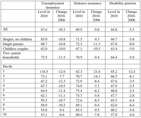
The level of the PTR is different for individuals going from different transfer systems (e.g. unemployment insurance or sickness insurance) Since the rules differ for different transfer systems the PTR for the individual also differs. Table 2.5 reports average levels in 2010 and changes between 2006 and 2010 in PTR:s by household type and decile for three transfer systems: the unemployment insurance system, the sickness insurance system and the disability pension system.1112 Deciles are defined on the basis of labour income.

       11

When interpreting average PTR:s and METR:s for the household types one should keep in mind that these differences may reflect differences in income.

12

In this report we do not calculate PTR:s for those who are on social assistance (“socialbidrag”, “försörjningsstöd”) since this is not a standard routine at the Ministry of Finance. Social assistance is means-tested against income net of the preliminary tax payment.

Table 2.5. Participation tax rates for different categories of non-employment

Unemployment insurance

Sickness insurance Disability pension

Level in 2010 Change 2010-2006 Level in 2010 Change 2010-2006 Level in 2010 Change 2010-2006 All 67.6 -10.3 69.9 -9.8 64.8 -5.3 Singles, no children 65.0 -10.8 71.5 -9.3 66.7 -5.8 Single parents 68.7 -10.8 72.3 -11.3 67.8 -8.0 Childless couples 62.0 -10.0 67.1 -10.5 63.4 -5.0 Two- parent households 72.5 -11.5 70.9 -9.4 64.4 -5.0 Decile 1 116.5 -12.6 62.3 -21.6 65.2 -12.4 2 73.1 -7.7 70.7 -14.1 66.5 -8.1 3 67.2 -12.3 72.9 -8.4 67.6 -3.5 4 67.7 -10.5 74.9 -7.1 67.9 -2.5 5 64.9 -11.4 75.4 -6.2 68.0 -2.5 6 62.1 -11.1 75.7 -5.8 67.7 -2.8 7 59.3 -10.7 72.6 -8.3 65.5 -4.4 8 56.9 -10.2 69.1 -9.4 62.6 -6.4 9 54.8 -9.4 65.5 -9.5 60.2 -5.6 10 53.1 -6.6 60.4 -7.8 57.0 -4.6  

Table 2.5 shows that the PTR:s for the unemployment insurance system have decreased across all demographic groups and income deciles. The mean level of the PTR has fallen from 77.8% in 2006 to 67.6% in 2010. The high PTR:s in the first decile can be explained by the fact that there is a minimum level in the unemployment insurance scheme. The unemployed person receives a minimum amount regardless of the income earned while at work. During the time period 2006 to 2010 the reduction in PTR:s was the largest in the 1st decile and the smallest in the 10th decile.

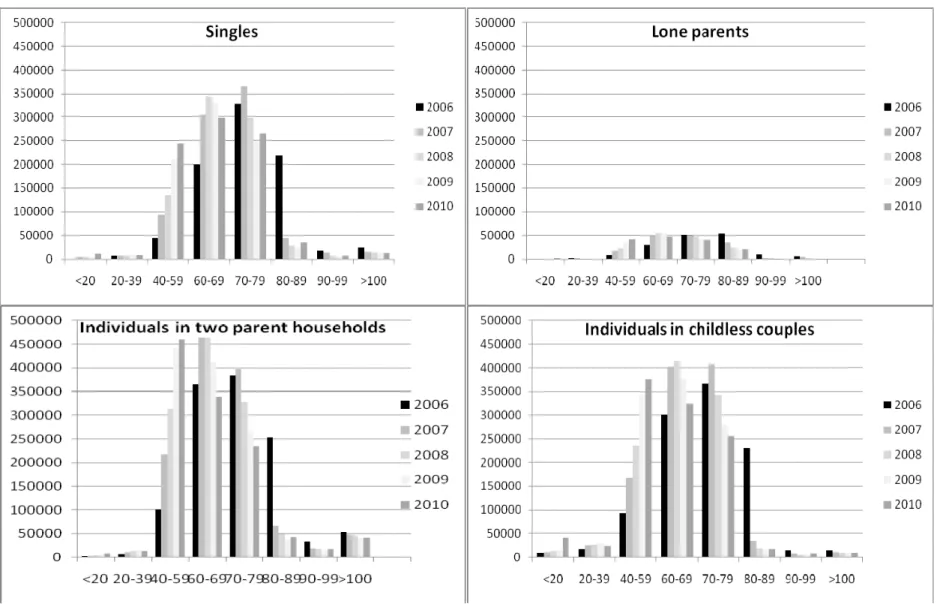
Figure 2.2 provides more information on the distributions of individuals in each PTR interval through 2006 to 2010. The population totals have been estimated using population weights. Among singles it is striking that over 200,000 singles faced PTR:s in the range 80-90% in 2006, while only about 30,000 individuals were doing so in 2010. The same pattern can also be discerned for ‘individuals in childless couples’, ‘single parents’ and ‘individuals in two parent households’.

Table 2.5 further reveals that the evolution in sickness insurance PTR:s has been quite similar as in the unemployment insurance case. In the case of sickness insurance the reduction has been more concentrated on deciles 1 and 2, however. PTR:s for the disability pension

have evolved slightly differently. Here the average level was lower in 2006. On the other hand, the decrease has been considerably lower than in the other two systems. Interestingly, there have been no major reforms in the disability pension during the period of study. The reductions in PTR:s shown in Table 2.7 can therefore largely be ascribed to the introduction of the EITC. It is interesting that the reductions in PTR:s is considerably lower than in the unemployment insurance system and in the sickness insurance system, where PTR:s have

been lowered both through changes in the social insurance system and in the income tax

system.

How high are the participation tax rates in a comparative context? The seminal study that brought participation tax rates to the centre stage of analysis is that by Immervoll et al.(2007). It already contained simulation results for participation tax rates across EU countries based on EUROMOD analysis and 1998 tax rules. Then Sweden had the second highest participation tax rates (after Denmark), ranging from 70% to 75% , with the highest figures for the lowest decile. A more up-to-date comparison is available in Immervoll and Pearson (2009, Figure 1)13 who depict the participation tax rate for a person moving from unemployment to full-time work at 2/3 of the average wage in 2005. For such a person, the participation tax rate was above 75% in Sweden (the third highest figure across the OECD countries), whereas for a typical country in continental Europe, the participation tax rate was around 65%. Participation tax rates were lower still in countries with less redistribution (such as the US). Therefore, before the introduction of the EITC in Sweden, the participation tax rates were among the highest in the world, but now the relative position of Sweden has probably improved somewhat in this aspect. While discussing trends in average tax rates (taking into account both the tax and transfer system) between 2000 and 2009, the OECD (2009) remarks that ‘the most significant reductions affecting all of the family types are noted in Sweden (p.130)’.

4.3.2. Marginal effective tax rate

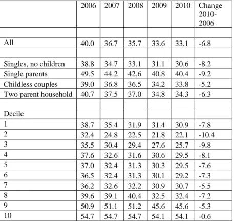
In addition to the statutory tax system METR takes account of all the transfer systems of an individual at a certain income level. Table 2.6 reports the evolution of METR:s 2006-2010. Note that METR:s on average are higher in the first decile than in the second decile. This is an effect of the transfer system. There has clearly been a decrease in METR:s for all, except for

       13

This study also offers an in-depth review of different types of in-work benefits currently in place in OECD countries.

the top decile, where instead METR:s have been fairly constant through 2006 to 2010. In principle, for higher incomes the entire METR is due to the statutory tax system. As the top marginal tax rates were constant during the period of study the average METR in the top decile has also been fairly constant.

Figure 2.3 shows the number of individuals in each METR interval from 2006 to 2010. In particular, it is striking that the number of single parents with very high METR:s diminished during the last four years. One should keep in mind that the METR:s reported in Table 2.6 do not include the value added tax (VAT) and payroll taxes. If one also takes these indirect taxes into account the METR:s are higher. As discussed in Appendix 1, METR of 0.29 reported in Table 2.6 translates to METR of 0.48 if one also takes indirect taxes into account.

Table 2.6. Marginal effective tax rates 2006-2010

2006 2007 2008 2009 2010 Change 2010-2006 All 40.0 36.7 35.7 33.6 33.1 -6.8 Singles, no children 38.8 34.7 33.1 31.1 30.6 -8.2 Single parents 49.5 44.2 42.6 40.8 40.4 -9.2 Childless couples 39.0 36.8 36.5 34.2 33.8 -5.2 Two parent household 40.7 37.5 37.0 34.8 34.3 -6.3 Decile 1 38.7 35.4 31.9 31.4 30.9 -7.8 2 32.4 24.8 22.5 21.8 22.1 -10.4 3 35.5 30.4 29.4 27.6 25.7 -9.8 4 37.6 32.6 31.6 30.6 29.5 -8.1 5 37.0 32.4 31.3 30.3 29.5 -7.6 6 36.5 32.4 31.3 30.1 29.2 -7.3 7 36.2 32.6 32.2 30.9 30.7 -5.5 8 39.6 39.1 40.4 32.5 32.4 -7.2 9 50.9 51.1 51.2 45.6 45.6 -5.3 10 54.7 54.7 54.7 54.1 54.1 -0.6

4.3.3 Summary of METR and PTR simulations

Taken together, this descriptive microsimulation exercise shows that both PTR:s and METR:s have decreased in Sweden in the last couple of years. PTR:s for unemployment insurance is still falling in income, which could be problematic given that low income earners often are

considered to be more responsive along the extensive labour supply margin (see the discussion in Section 4). We also note that METR:s decreased for some low income groups – among single mothers there has been a clear reduction 2006-2010. Interestingly, not much happened to the METR applying to top income earners. The top METR will be further discussed in Section 5.2.

Figure 2.2. Participation tax rates if the individual receives unemployment insurance benefits if not working. Estimated number of individuals (vertical axis) with a PTR in a certain interval (horizontal axis).

3. Lessons from optimal tax theory

Optimal tax theory, initiated by the Nobel-prize winning economist James Mirrlees (1971), provides a robust base for analysing the inherent trade-off between distributional concerns and efficiency aspects mentioned in the introduction. Optimal taxation does not start with some arbitrary principles, such as “it is always good to have a broad tax base and low tax rates” or that “one should tax consumption, not income”, a statement behind some flat tax proposals, for example. Instead it starts from a specification of societal preferences (captured via a social welfare function) and then examines which tax structures and tax rates could best achieve these social aims (Banks and Diamond 2010). The resulting tax structures may sometimes be quite complicated, but they certainly serve – with suitable modifications such as administrative constraints – as a yardstick to which actual tax systems can be compared.

This framework embeds the problem of designing low-income support (transfers to those who do not work or work very little) into the general problem of choosing an optimal income tax system. The optimal system typically includes a guaranteed minimum income for those who do not work and rising average tax rates with increasing income.

3.1 The basic analysis

The analysis in Mirrlees (1971) requires modelling of the social preferences, underlying pre-tax income differences, assumptions on the revenue requirement of the government, and ideas on the distortions the tax system creates. The latter are often modelled via labour supply decisions, where higher taxes reduce labour supply; but in a more recent analysis, other distortions are examined as well. Because of higher tax rates, individuals may exert less effort per working hour, which would then be reflected as a lower hourly wage rate, or acquire less formal education. High tax rates can also diminish the incentives to switch to better-paying jobs, which would be desirable from the point of view of enhancing overall productivity in the economy. In principle, all these distortions are captured in the notion of taxable income elasticity discussed in more detail in Section 4.2 – under certain conditions, taxable income elasticity is a sufficient statistic of all tax-generated distortions.

Optimal tax results have been reviewed by e.g. Tuomala (1990) and Salanié (2003). According to the basic analysis, the overall tax rates tend to increase if

 pre-tax income distribution becomes more unequal – this is the distribution the government attempts to correct

 labour supply decisions become less elastic – the distortions the tax system creates become smaller

 the government’s preferences become more egalitarian

 the revenue requirement of the government increases

These general principles are intuitive, but they tell relatively little about the actual marginal tax rate at different income levels, i.e. about the shape of the marginal tax rates over gross income.

A key factor affecting that shape is the underlying income (or skill) distribution. Marginal tax rates ought to be high in those areas of skill distribution where there are few taxpayers, because then the number of people facing severe distortions is limited. On the other hand, marginal tax rates should be high at those income levels above which many taxpayers are situated. For these people, the high marginal tax rate at a smaller income level only creates an income effect, and hence it is not distortive. The marginal tax rate at a given income also depends on the societal value of additional income to persons at that income level: with redistributive preferences, the marginal value of additional income is declining in gross income. And of course, the optimal marginal tax rate for a given skill group is also affected by the magnitude of the taxable income elasticity in this skill group.

These observations imply that optimal marginal tax rates can easily reach high levels at small incomes: at these income levels, there are few taxpayers, but many taxpayers are situated above them in the income distribution. This also means that transfers given to those who do not work at all are tapered off relatively rapidly (although below in Section 3.3. we note that this result does not hold if labour force participation is particularly elastic). Optimal marginal tax rates could then be relatively low at middle income levels (where the majority of tax payers are situated) and they would rise again for high enough income levels (because then they affect fewer persons and the social marginal value of their income is small). This would then lead to a U shaped marginal income tax rate curve over income (Brewer et al.2010).1415

       14

However, the study of the shape of optimal marginal tax rates is quite complicated and Tuomala (2010) derives tax rates that are fairly flat for reasonable assumptions about income distribution.

15

If the skill distribution is bounded from above, the marginal tax rate at the top should be zero. However, this result is a technical curiosity and of no relevance to practical tax policy: there is no way to know what would be

One issue not studied in the analysis above is income uncertainty. Real-world educational decisions to acquire income-earning abilities entail a substantial amount of uncertainty on, for example, the returns to education. Progressive taxation combined with a social security system provides a kind of insurance system against negative realisations of income shocks, which is valuable to individuals. These concerns tend to increase the desired progressivity of the tax system (Mirrlees 1974, Pirttilä and Tuomala 2007).

3.2 Optimal tax rate at the top of the distribution

A particular question concerns the appropriate marginal tax rate at the highest incomes, i.e. at the top. One approach is to try to find the level of the highest marginal tax rate which would raise the maximum amount of tax revenues. This notion of the top tax rate is consistent with a Rawlsian social welfare function where the welfare effects of the rich do not count, all that matters is the tax revenue that can be collected from them (to distribute to those who are less well off). It can be also defended on the grounds that with a high level of income, the social valuation of additional income for that person is likely to be small, at the limit negligible.16

The revenue-maximising top tax rate will only depend on the distortions taxes create and on the number of persons at the top of the distribution, i.e. how large the income differences are. The consensus among most tax economists is now that the relevant distortion at the top of the income distribution is the response in taxable income. This notion covers not only labour supply decisions, which are likely to be of minor importance for this part of the population, but also issues such as tax avoidance, a more relevant margin for these persons. The optimal tax rate at the top is the higher, the less the taxable income of top-income earners reacts to tax increases. The optimal tax rate is also the higher, the more unevenly the pre-tax income is distributed.

3.3 Taxing low incomes

The analysis described above builds on the traditional Mirrlees approach, where individuals can freely select hours of work – even a couple of hours in a week – with no additional constraints. The bulk of the recent empirical work suggests, however, that in reality individuals typically work either 0 hours, take a part-time job (with e.g. 20 hours a week) or

       the highest possible actual skill level (see e.g. the discussion in the preface in Mirrlees (2006). See also the discussion in Saez (2001).

16

they work full time. It appears that there are significant fixed costs in participating in the labour market and to overcome these, those who do work do not typically supply a few hours of work. Restrictions on the chosen hours may also arise from the employers’ side. This so-called extensive margin, as opposed to choosing the number of hours conditional on working (the intensive margin), has also been found more elastic for some groups of workers (see the discussion in Section 4).

A fairly elastic extensive margin has two important potential consequences (Saez 2002). First, the optimal transfers given to those who do not work but would be able to do so is substantially reduced. Second, the marginal tax rates for small incomes are also reduced; it is

also possible to optimally subsidise labour supply for low-income earners.17 These

observations lend support to the so-called in-work benefits or making-work-pay policies that were first implemented in the Anglo-Saxon countries (the EITC in the US and the WFTC in the UK) and that have now become popular in other welfare states as well. In these policies, transfers are not only given to the unemployed but also to workers with low incomes.

An alternative complication is a situation where individuals differ in both their income-earning abilities and tastes regarding the valuation of leisure. One approach then is responsibility sensitiveness: individuals should be held responsible for those features that are under their control (tastes) but they should be compensated for differences that are beyond their control (innate skill differences). Fleaurbaey and Maniquet (2006, 2007) introduce this notion to optimal tax analysis. They point out that favouring the hard-working low-skilled further supports the idea of in-work subsidies.

3.4 Tagging

The discussion above only used one source of information (on income) in designing tax policies. If individuals differ with respect to other relevant observable characteristics that are also correlated with income-earning abilities, the government could also base its tax and transfer policy on this information. This idea is known as ‘tagging’ and it was first examined by Akerlof (1978). An example might be that there could be two groups, a disadvantaged one and a fully able one. If the disadvantage is clearly observable and if people cannot themselves affect their disadvantages, the government can easily design separate tax schedules for the two groups. If information on this categorical information or the ‘tag’ or is observed

       17

The same outcome is, however, found when the government minimises the income poverty of those below the poverty line and pays no attention to the disutility of labour (Kanbur et al.1994).

erroneously or if people can partially overcome their disadvantages, the problem obviously becomes more complicated. In comparison to a solution where information on disability is not used, separate tax and transfer schedules allow more redistribution for the disadvantaged or smaller tax distortions or both (Immonen et al.1998). One policy relevant application of tagging is age-contingent taxation; an idea that in the Swedish system is used in payroll taxation and in personal taxation (higher tax credit for elderly workers).

3.5 Focusing on households rather than individuals

The discussion above focused extensively on individuals, whereas the issues related to the taxation of couples was omitted. This is serious shortcoming, since real tax policies must deal with this issue in fact for the majority of the taxpayers. Kleven et al.(2009a) offer a very useful study of family taxation where the secondary earner only chooses whether to work or not, whereas the primary earner also chooses the hours of work. They show that the marginal taxes are higher at the optimum for the secondary earner whose spouse earns more. This is so because conditional on spousal earnings, two-earner couples are better off than one-earner couples. Then the government would like to redistribute towards one-earner couples, and the value of this redistribution is higher at the bottom of the distribution. This rather unexpected result is actually compatible with many real-world tax and transfers systems, where individuals are taxed separately, but transfers are means-tested against family income. The tapering off of transfer payments then creates the higher effective marginal tax rates for couples where the primary earner earns less.

3.6 The role of salience in the tax system

The standard economic analysis of taxation assumes that individuals are fully aware of the tax code and can optimise their labour supply and other decisions without any friction. Recent work in behavioural public economics – which draws heavily on findings in psychology – has, however, demonstrated that these assumptions are not necessarily innocuous.

For example, Chetty and Saez (2009) examine how information provision on the EITC in the US affects labour supply decisions. According to earlier studies, workers eligible for the EITC typically know about the existence of the subsidy system, but they are not fully aware of all the effects of the programme on effective marginal tax rates in its phasing-in and phasing-out regions. The authors therefore designed an experiment where the persons assisting the individuals to prepare their tax files advise the taxpayers about the EITC system

so that half of the taxpayers get the treatment and the other half was randomly assigned to the control group. After the experiment it turned out that not all tax preparers had complied with the experimental design (they preferred to always encourage their clients to earn more even if that would have led to the phase-out region of the subsidy). The clients of the complying tax preparers were statistically significantly less likely to report very small incomes (presumably to qualify for the phase-in part of the system). Since the earnings are reported by a third party (their employers) and they are therefore difficult to falsify, this change probably reflects a real behavioural change in labour supply. Chetty and Saez point out that information appears to have a quantitatively important effect, roughly comparable to a one third increase in the monetary value of the EITC.

A related idea, but one that goes in another direction, is related to the notion of hidden taxes. Evidence seems to suggest (Blumkin et al.2009) that individuals find it harder to understand the tax burden created by indirect taxes as opposed to the more salient direct income taxes. This would mean that some of the harmful behavioural effects of taxation could actually be lessened by hiding part of the tax burden in instruments such as indirect taxes and the employers’ social security payments.

Chetty (2009) highlights the role of decision-making frictions for tax analysis. He seeks to build a bridge between diverging lessons from micro-level empirical tax analyses (that typically find modest behavioural responses to tax changes) and to macro-level studies, such as Prescott (2004), claiming that taxation could have major effects on the overall economy when one considers all possible channels of influence. The existence of frictions can explain why changes to small tax reforms may be negligible if the gains from changing one’s behaviour exceed the costs of re-optimisation and therefore people do not find it worthwhile to react. However, large tax differences, which exist, for example, between countries, lead to re-optimisation and reactions among the taxpayers. Chetty et al.(2010) find support for this idea using Danish data on income tax changes where elasticities estimated from the larger tax changes tend to be higher than elasticities estimated only from small changes (more on this below in Section 4).

Taken together, the discussion above means that to create major impacts on labour supply, in-work-benefits should be sizable and easily understandable in order to be likely to actually affect labour supply.

3.7 Taxation in an open economy: the role of migration

A common concern is that the increasing mobility of the highly skilled may lead to tax competition for high-income taxpayers similar to that in the location decisions of multinationals. The Nordic countries are especially vulnerable to this kind of tax competition, since higher education is virtually free of charge, wage dispersion is relatively narrow and labour income is taxed more progressively than in some competitor countries, notably the Anglo-Saxon countries. Even if the mobility of high-income taxpayers is relatively small, that would still lead to large losses in tax revenues since these individuals are large net payers to the government.

While migration decisions depend on many other things than simply tax rates, there is still some evidence that countries have attracted highly skilled individuals with lower taxes on labour (Egger and Radulescu 2008)18, and these forces could intensify in the future. A simple intuition suggests that the progressivity of labour income taxation must then be reduced. This intuition is confirmed by a fully-fledged optimal tax analysis by Simula and Trannoy (2010) who show that when setting the optimal marginal tax rate, the government must consider an additional responsive margin, emigration. If emigration is a concern for France, it is certainly also so for the Nordic countries. Thus the revenue-maximising top tax rate could be somewhat below the one derived in a closed economy setting.

3.8 Other tax instruments

Is it sufficient to confine redistribution to be dealt with in income taxation, or should the government use other tax instruments (notably commodity taxes and the pricing of publicly provided goods) in its redistributive policy? The key to this answer is the role of information: if, for example, commodity purchases provide additional information on the underlying skill of the household (that is not revealed by gross income levels), commodity taxation can have a potentially useful role in tax policy.19 For example, if preferences differ so that those who work more, holding income constant, consume more of some goods than those with more leisure, introducing a small subsidy to goods that in conjunction with labour supply can increase welfare by making labour supply more desirable and thereby reducing the distortions created by the income tax. Similarly, goods that are complementary to leisure ought to be taxed, and publicly provided goods that support labour supply (such as day care) should be

       18

Kleven, Landais and Saez (2009b) find a large migration elasticity for a specific group (international-level football players); of course, the external validity of this finding is open.

19

This large literature was started by Christiansen (1984), Boadway and Keen (1993) and Edwards, Keen and Tuomala (1994). For an impressive recent contribution, see Blomquist et al.(2010).

provided at a reduced fee. However, if the commodity purchases at a given income level do not depend on labour supply, differentiated commodity taxation is not needed from a labour supply perspective (Atkinson and Stiglitz 1976, Kaplow 2006).

Crawford et al.(2008) examine this issue empirically using UK data. They confirm the intuition that commodity purchases do indeed differ depending on labour supply decisions (consider for example travel costs that arise from commuting), but they claim that the empirical magnitude of these effects is modest. Taking into account administrative costs would then speak in favour of uniform commodity taxation. However, there is some evidence that at least housing and capital income are negatively related to labour supply (Gordon and Kopczuk 2008) and that the use of day care services has a positive relation to it (Pirttilä and Suoniemi 2010), suggesting that gains could be derived from specific considerations of these items in supporting labour supply.

An especially relevant issue is the tax treatment of services that are substitutes for household production (such as cleaning and home repair services). The analysis in Kleven et al.(2000) confirms the intuition that such services should be favoured by the tax system if doing so significantly increases labour supply (people can work full time if they do not need to repair their houses themselves).20 Applied to the real world, two key issues in favouring these services are to what extent tax cuts are actually related to reductions in consumer prices and tax evasion. Firstly, while the supply, for example, of cleaning services is probably quite elastic, the availability of skilled house repairers can be scarce, and then tax reductions in the latter sector perhaps mainly lead to a rise in pre-tax prices and therefore the absolute demand for these services does not necessarily increase (Uusitalo 2005). This would mean that one needs to carefully select the services where the scope for actual increases in the equilibrium amount is large. The case for subsidising the services is also the higher, the more their supply is low-skilled labour intensive – then subsidies are an indirect way to increase the relative wages in the sector (Naito 1999). However, even if the official use of skilled house repairers would not appear to increase, it might be the case that moonlightning could go down, and hence the tax revenue loss in granting the deduction can be (at least partly) offset. The trouble is that the empirical analysis of the shadow economy is by definition difficult.

Finally, although not a tax instrument, an important additional way to affect the distortions created by the tax and transfer system is activation requirements for those who obtain unemployment assistance or other transfers. Activation policies mean that in order to

       20

This interpretation is also compatible with lessons from such optimal commodity tax analysis where the time use of consumption is taken into account (Boadway and Gahvari 2006).

be eligible for the benefits, the unemployed must participate in training or guided job search programmes. This implies that the unemployed do not enjoy much more pure leisure than workers do and the potential moral hazard problems inherent in unemployment insurance systems (as in any insurance situation) can be mitigated. Therefore, activation requirements can be regarded as a substitute for reducing the guaranteed income (or transfers): both policies can increase the willingness to take a job, but with different implications for the income level of the unemployed (Andersen and Svarer 2007).

4. Empirical findings on the employment effects of labour income taxation

4.1 Empirical studies on labour supply

The idea that taxes can influence the amount of work done through labour supply decisions was already mentioned in the introduction. Recall now that that an increase in the marginal tax rate has two effects on the number of hours worked:

(i) The substitution effect is the change in labour supply that is due to the change in the relative price between consumption and leisure: when leisure becomes cheaper the agent ‘purchases’ more leisure (i.e. works less). Hence, this effect works in the direction of lowering labour supply.

(ii) The income effect is the change in labour supply that occurs owing to the fact that disposable income has decreased. If leisure is a normal good21 the individual will supply more work hours as a consequence of the imposition of the tax. Intuitively, she needs to work more hours to achieve a given level of utility.

Accordingly, the substitution and income effects typically work in opposite directions and the net effect is theoretically undetermined. Empirical evidence is needed to tell in which direction the net effect goes. Income effects can also arise when the individual’s non-labour (the amount of money that she can consume when she works 0 hours) changes.

Perhaps the most important labour supply decision is the participation decision. The individual chooses to participate if the utility level at 0 work hours, where she only consumes her non-labour income, is less than the utility level she would attain if she chose to work.

       21

Note that participation may entail significant fixed costs of work, such as commuting, child care costs etc. that can imply that the individual either chooses to work a lot of hours per week (from 20 to 40) or then not at all. The incentives for participation in Sweden were measured above in Section 2 in the form of participation tax rates.

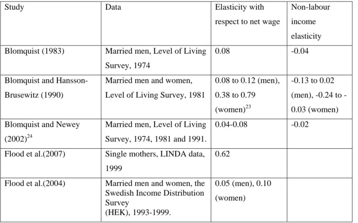
The table below collects results from studies on labour supply conducted on Swedish data.22As often in economics, we express the responsiveness of labour supply as elasticities: labour supply elasticity with respect to the net wage measures the total percentage change in hours of work when the take-home pay (1-marginal tax rate) increases by one per cent. The non-labour income elasticity measures in turn the percentage change in hours of work when the person’s non-labour income increases by one per cent.

Table 4.1: Some structural Swedish studies on labour supply

Study Data Elasticity with

respect to net wage

Non-labour income elasticity Blomquist (1983) Married men, Level of Living

Survey, 1974

0.08 -0.04 Blomquist and

Hansson-Brusewitz (1990)

Married men and women, Level of Living Survey, 1981

0.08 to 0.12 (men), 0.38 to 0.79 (women)23 -0.13 to 0.02 (men), 0.24 to -0.03 (women) Blomquist and Newey

(2002)24

Married men, Level of Living Survey, 1974, 1981 and 1991.

0.04-0.08 -0.02 Flood et al.(2007) Single mothers, LINDA data,

1999

0.62 Flood et al.(2004) Married men and women, the

Swedish Income Distribution Survey (HEK), 1993-1999. 0.05 (men), 0.10 (women)        22

. A related recent survey – which involves somewhat more technicalities -- of Swedish studies on labour supply and taxation is provided by Aronsson and Walker (2010).

23

Interestingly, Blomquist and Hansson-Brusewitz found similar elasticities for males and females when evaluating the elasticities at the same level of hours and wages. These results run counter to the common notion that female labour supply is more responsive to taxes than male labour supply.

24

Liang (2009) extends the estimation framework of Blomquist and Newey (2002) by allowing for non-participation in the labour force. This is done on Swedish survey and register data, again from the Swedish Level of Living Survey (the 1974, 1981, 1991 and 2000 waves). Liang studies how married women respond to income taxation and finds an aggregate uncompensated wage elasticity of 0.9 for marginal tax changes in low and medium income brackets. These elasticities are roughly equally driven by the participation margin and the continuous hours margin. In high income brackets, he finds an elasticity of 1.4.

A common result in labour supply studies is that women are found to have higher wage elasticities than men -- both along the participation margin and the continuous hours margin. This is not specific to Sweden, but is true for most countries. Historically, there has been considerably more variation over time in female participation rates and also in the choice on working hours as many women have chosen to work half time. In Sweden, it has historically been the case that participation among men is high and that most men work full time. Whether the quantitative constraints (fixed hours contracts) should be seen as an explanation for or an outcome of the low labour supply elasticities for males is an open issue.

Labour supply models can also be used to study the effects of policy changes. Ericson et al.(2009) offer an ex ante simulation – meaning a forecast on likely effects of a policy change

– of the Swedish EITC reform as of 2007.25 The data comes from the 2006 wave of LINDA.

While taking the tax law changes implemented in 2007-2009 into account the authors conclude that the reforms led to an increase in labour supply – both via the participation and the hours-of-work decision. Sacklén (2009) uses a similar model and estimates labour supply for different demographic groups based on HEK data from 2004. He finds quite low participation elasticities (0.12 for women and 0.08 for men).26 His simulations suggest that men should increase their working hours by 1.9 percent and women by 2.8 percent in response to the reforms occurring between 2007 and 2009. Most of the response is driven by changes along the extensive margin. Aaberge and Flood (2008) also evaluate the 2007 reform for single mothers. The authors find an increase in labour supply among single mothers, which makes the reform almost self-financing for this group.

The abovementioned studies are all part of the so-called structural tradition of labour supply estimation. These works aim at estimating individuals’ preferences for leisure and consumption so that it is possible to simulate the welfare consequences of actual tax policy reforms. Some empirical researchers, however, tend to think that some of the statistical assumptions inherent in this tradition are problematic.

Since the 1990’s a new quasi-experimental literature on labour supply and taxes has emerged. To a large extent, this literature centres on various earned income tax credit policies. A common strategy has been to compare labour market outcomes of eligible and non-eligible to income tax credits with data from before and after a policy-reform and employ the so-called difference-in-difference method. Simplistically put, the basic idea behind this method is

       25

Flood and Ericson (2009) assess the optimality of the Swedish tax system using this method. 26

Here the participation elasticity is defined as the percentage change in the number of persons in employment in response to a percentage increase in the financial gain for working full time.

to compare the average level of working hours (or participation) for a treatment group and a control group before and after a policy reform. The validity of the results from these studies typically depends on other sets of assumptions when compared to works in the structural tradition.

The EITC in the U.S., which in contrast to its Swedish counterpart is a refundable tax credit, dates back to 1975. A sequence of expansions has taken place since then, most importantly in 1986, 1990, 1990 and 1993. In a well-known paper Eissa and Liebman (1996) analyse the effects of the 1986 EITC expansion on the labour supply of single women with children. The 1986 reform affected labour supply incentives for this group, but did not affect incentives for single women without children. Eissa and Liebman compare the relative labour supply outcomes of single women with and without children. They find that the reform increased labour force participation by up to 2.8 percentage points among single women without children.

These main results for the U.S. – that there is a sizeable effect from the EITC along the participation decision but that that there are only small, if any, effects on the hours of work on those who were already working – are not specific to the Eissa and Liebman (1996) paper, but echo as a general theme in a wide variety of research on the EITC.27

Empirical research on Swedish data on labour supply responsiveness to income taxation has traditionally not been conducted in this difference-in-differences setting. An exception is Klevmarken (2000), who utilizes the Swedish tax reform act of 1991 to study labour supply among both males and females on a smaller panel data set (HUS). Klevmarken’s results are broadly consistent with the results obtained in other studies on Swedish labour supply. Females appear to be more responsive than males. Women increased their working hours by 10 per cent owing to the reform, whereas working males probably changed their working hours little.

Selin (2009) exploits the 1971 move from a joint to a separate system in family taxation to examine how sensitive the employment decision is to changes in the net-of-tax share (1- the average tax rate) and the non-labour income. Before 1971 the earnings of each spouse were added together and taxed according to a steeply progressive tax schedule. This meant that the average tax rate for the housewife was a function of the ‘last-krona’ marginal tax rate of her husband. After the reform, the link between the husband’s earned income and the wife’s average tax rate was in principle abolished. The study uses a LINDA sample of 18,069

       27

wives. Selin obtains statistically significant estimates of the employment elasticities both with respect to the net-of-tax share and with respect to non-labour income. The former is 0.46 and the latter is -0.14. The simulations suggest that employment among married women would have been 10 percentage points lower in 1975 if the 1969 statutory income tax system had still been in place in 1975.

4.2 Taxable income elasticity

In the labour supply literature it has been implicitly assumed that the choiceof working hours

is the relevant margin to study if one is to understand how income tax reforms affect

individual behaviour. However, it is not farfetched to believe that individuals might respond to income tax reforms by adjusting their behaviour along other margins. Suppose that the marginal tax rate decreases. Then the individual might increase her work effort per hour and thereby increase her hourly wage rate. Another possibility is that she accepts job offers that she would otherwise reject or that she puts more effort into wage bargaining. She might also lower the resources spent on tax avoidance or tax evasion since the marginal gain from sheltering money decreases on the margin.

All these effects are captured in the taxable income the individual supplies. Therefore, the elasticity of taxable income with respect to the net-of-tax rate (1- marginal tax rate) is a wide measure of the distortions taxation creates (Feldstein 1995, 1999). In contrast to individuals’ preferences between work and leisure that underlie labour supply behaviour, taxable income elasticity, however, is not a parameter that would be beyond the government’s control via other means than taxation. Slemrod (1998) points out that making avoidance more difficult by better monitoring and detection, for instance, is one way to reduce the elasticity of taxable income at a given tax level.

Much of the evidence on taxable income elasticity is based on examining how individuals react to tax reforms where different taxpayers face different rate changes. One key issue is how to take into account non-tax factors affecting income growth. If these are not accounted for, the researcher may incorrectly ascribe income growth to tax changes.

Saez et al.(2009) survey the international literature on the topic. An important study by Gruber and Saez (2002) obtained a preferred estimate of the overall taxable income elasticity of 0.4 when using U.S. data from the 1980’s. This is an estimate well above the traditional labour supply elasticity estimates obtained for married males (that has usually been estimated to be around 0.1). However, it appears as if most of the response stems from changes in

deduction behaviour. When Gruber and Saez estimate the response in a broader income measure that does not include deductions the overall elasticity reduces to 0.12 and is insignificantly different from 0. The importance of deductions has also been confirmed by Kopczuk (2005), who disentangles taxable income responses to changes in marginal tax rates and in changes in the tax base.

Another interesting lesson from the U.S. literature is that it appears as if the response is concentrated on the top of the income distribution. This is natural, since low and middle income earners receive more income in the form of wage income that is not so easily manipulated. High income taxpayers have more ample opportunities to engage in different kinds of tax avoidance strategies (like changing the form of compensation).

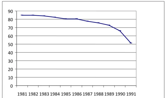
There are also a number of Swedish studies on taxable income elasticity. Many base their analysis on the 1991 tax reform, when a dual income tax system (labour income is taxed progressively whereas capital income is subject to a proportional tax rate) was introduced in Sweden (Agell et al.1998). The reform combined sharp cuts in top marginal tax rates with base broadening measures. The pre-reform five-bracket central government tax system with marginal tax rates ranging from 0 to 42% was replaced with a two-bracket central government tax with two brackets, where the marginal tax rates were set at 0 and 20 %. Since the mean local tax rate was around 31 % during this period, the top marginal tax rate applying to labour income fell from 73 % in 1989 to 51 % in 1991. However, if one considers the whole series of income tax reforms occurring in Sweden during the 1980’s the decline in top marginal taxes is even more striking. As can be seen from Figure 4.1 the top marginal tax rate amounted to 85 % in 1981.  

Figure 4.1. Top marginal tax rates 1981-1991 in percent by year.

Different taxpayers were affected differently by the 1991 reform. Those at the top of the income distribution experienced large tax cuts, whereas those at the bottom of the income distribution were subject to considerably smaller tax changes. It is noteworthy that those in the middle-income ranges also faced quite large marginal tax cuts. This is because the pre-1991 central government tax system was very progressive, even at modest income levels.

There are several papers that examine the taxable income response to the 1991 reform from different angles. These are summarized in Table 4.2 below.

Table 4.2: Some Swedish studies on the elasticity of taxable income

Study Data Elasticity

Selen (2005) Household income survey (HINK) 0.2 – 0.4

Hansson (2007) LINDA 0.4 – 0.5

Ljunge and Ragan (2006) LINDA 0.35 – 0.6

This basic analysis is complemented by Gelber (2010), who allows spouses to respond to each other’s marginal tax rates. The own elasticity is the percentage change in own earned income to a percentage change in the own net-of-tax rate. The cross elasticity is the

0 10  20  30  40  50  60  70  80  90  1981 1982 1983 1984 1985 1986 1987 1988 1989 1990 1991