NBER WORKING PAPER SERIES
USING TAX RETURN DATA TO SIMULATE CORPORATE MARGINAL TAX RATES
John R. Graham Lillian F. Mills Working Paper 13709
http://www.nber.org/papers/w13709
NATIONAL BUREAU OF ECONOMIC RESEARCH 1050 Massachusetts Avenue
Cambridge, MA 02138 December 2007
We thank Jennifer Blouin, Mark Evans, Michelle Hanlon, Oliver Li, George Plesko, Jim Poterba, Clemens Sialm, Doug Shackelford, Terry Shevlin, Joel Slemrod, Jerry Zimmerman and participants at the NBER July 2006 and December 2006 Conferences on Financial Reporting and Tax Policy for their comments. We appreciate excellent research assistance from Brett Hollenbeck (U.S. Department of Treasury), Jonathan Mable (UBS, formerly U.S. Department of Treasury) and Casey Schwab (University of Texas). The U.S. Treasury Department provided confidential tax information to Mills during her 2005-2006 appointment as a Stanley Surrey Senior Research Fellow at the Office of Tax Analysis. None of the confidential tax information is disclosed in this treatise. Statistical aggregates are presented in the tables so that a specific taxpayer cannot be identified. The opinions expressed are those of the authors and do not necessarily represent positions of the U.S. Department of the Treasury. The views expressed herein are those of the author(s) and do not necessarily reflect the views of the National Bureau of Economic Research.
© 2007 by John R. Graham and Lillian F. Mills. All rights reserved. Short sections of text, not to exceed two paragraphs, may be quoted without explicit permission provided that full credit, including © notice, is given to the source.
Using Tax Return Data to Simulate Corporate Marginal Tax Rates John R. Graham and Lillian F. Mills
NBER Working Paper No. 13709 December 2007
JEL No. G32,H25,M41
ABSTRACT
We document that simulated corporate marginal tax rates based on financial statement data (Shevlin 1990 and Graham 1996a) are highly correlated with simulated rates based on corporate tax return data. We provide algorithms that can be used to estimate the book or tax simulated rates when they are not available. We find that the simulated book marginal tax rate does a better job of explaining financial statement debt ratios than does the analogous tax return variable and discuss how the book simulated rate is likely to be an appropriate measure in settings with global, long-term considerations.
John R. Graham Duke University
Fuqua School of Business One Towerview Drive Durham, NC 27708-0120 and NBER
[email protected] Lillian F. Mills
University of Texas
McCombs School of Business Austin, TX 78712
1. Introduction
The marginal tax rate (MTR) is an important input into many corporate decisions. For example, high marginal tax rate firms are hypothesized to use more debt, restructure via Chapter 11 when in distress, and participate in tax shelters. Low marginal tax rate firms are thought to pay employees with deferred and/or stock compensation rather than salary, operate as corporations rather than partnerships, and lease rather than buy assets. The corporate MTR also is a key input into the cost of capital and, therefore, affects many capital budgeting decisions.1 Given the significance of these issues, it is important to measure corporate marginal income tax rates accurately and choose a rate appropriate to the research question.
Ideally, to test for tax effects, researchers would construct the tax variable(s) that managers use in their actual decision making. In theory, such tax rates should incorporate the effects of net operating losses (NOLs), projections of future income, and various features of the tax code (for all jurisdictions), as appropriate. For economic decisions that are tied to an incremental dollar of income or deduction, like those mentioned above, tax incentives should be measured by a marginal income tax rate.
In practice, much prior research has relied on simple static tax variables created from financial statement data, such as the presence of an NOL carryforward, to measure tax incentives. The value of a static variable is limited, however, when dynamic considerations are important, such as when a firm’s tax status is expected to change in the near future. Shevlin (1990) and Graham (1996a) address this concern by simulating
1
We measure the MTR as the present value of incremental taxes paid on an additional dollar of current-period income, consistent with Scholes et al.’s (2005) corporate income marginal tax rate. This measure of the MTR on the next dollar of income differs from the concept of the marginal effective tax rate on an investment, which is estimated as the expected pretax return minus the expected after tax return, divided by the expected pretax return. See Fullerton (1999) for a brief description.
marginal tax rates that capture important dynamic features of the tax code such as the effects of NOL carrybacks and carryforwards. While a simulated tax variable based on financial statement information (hereafter, the book simulated rate) is only an approximation of the theoretical, “true” tax variable that managers use in their actual decisions, it appears to be a reasonable proxy because it loads as expected in many economic settings (see Graham (2003) for a summary of findings). In addition, the simulated book MTR performs well in experiments that compare it to benchmark tax rates that are believed to capture important elements of the “true” tax variable.
In one such experiment, Graham (1996b) compares financial statement tax variables to a benchmark marginal tax rate that models dynamic features of the tax code and is based on “perfect foresight” future book income. He finds that the simulated book MTR is most highly correlated with the perfect foresight benchmark. In a second experiment, Plesko (2003) tests how closely book MTRs approximate a benchmark MTR that is based on tax return data. Plesko examines a small sample of homogeneous, single-entity firms, chosen to eliminate firms for which the reporting single-entity is likely to vary between financial and tax reporting. He uses 1992 data to form a static tax return tax rate benchmark against which to compare a collection of financial statement MTRs. Plesko finds that Graham’s (1996a) simulated book MTRs are the closest approximation to his benchmark static tax return MTR.
While the book simulated MTR performs well in these two experiments, there are still unanswered questions. In particular, how closely does the book simulated rate approximate a tax return benchmark that incorporates dynamic features of the tax code? Also, do the results validating the book simulated rate hold for large, complex
corporations for which tax and book consolidated entities differ? The answers to these questions are important because they relate to issues often studied by researchers and to companies that are responsible for much of the world’s economic activity.
Our paper fills this void by comparing, for a sample of large, complex firms, a collection of financial statement tax rates to a dynamic tax return MTR benchmark. In particular, we use a panel of confidential U.S. tax return data from 1992 to 2000 to simulate corporate income MTRs for the years 1998 to 2000. We compare these benchmark tax rates to a collection of financial statement MTRs to determine which is most highly correlated. As an alternative, we also benchmark against a simple static tax return MTR that is based on realized future taxable income.
We find that, among the candidate financial statement tax variables, the book simulated MTR is most highly correlated with the dynamic tax return benchmark, further validating the book simulated MTR. The book simulated rate also performs well when benchmarked against the static tax return variables that are based on realized future taxable income. We also identify the “second best” book variables, in this case, categorical variables that combine information about net operating losses and the sign of pretax income; however, as detailed below, the amount of correlation lost by relying on second best, and even which variable is second best, varies by setting and benchmark.2 Taking all this evidence together, we conclude that researchers should use the simulated rate when it is available. For situations where the simulated rate is not available, we report algorithms that researchers can use to estimate the simulated book MTR. We also provide an algorithm to estimate the simulated tax return MTR for settings where tax
2
For example, the superiority of the simulated rate is greater when comparing MTRs based on pre-interest income than it is for MTRs based on post-interest income.
returns provide the ideal data to measure corporate tax incentives.
Even though we use it as a benchmark, one should not assume that a tax return tax rate is the “true” tax variable that managers use when making all decisions. As we detail in Section 3, there are advantages and disadvantages to using tax return data in tax rate calculations. A key advantage of using tax return data is that they allow us to directly measure taxable income, which is difficult to estimate from financial statement data due to “book-tax differences.” When these differences are temporary (e.g., accelerated tax depreciation vs. straight line book depreciation), researchers can estimate taxable income by adjusting book income for deferred taxes. When the book and tax differences are not temporary (e.g., fines or some stock option deductions), researchers are less able to adjust financial statement data for book-tax differences, making tax return data appear superior. However, tax return based measures are not without weaknesses as proxies for the “true” marginal tax rate. For one thing, due to differing consolidation rules, financial statement and U.S. tax return data do not always represent the same entity.3 In some situations, managers are likely to take actions relative to the firm’s global operations (which are often best represented by book data), rather than relative to domestic-only operations (often best reflected by U.S. tax return data).
To put this point in perspective, and to place our paper within the literature, consider which tax rate variable might be preferred in different settings (as summarized in Figure 1).4 The figure categorizes settings that involve worldwide vs. domestic
3
The U.S. tax return includes only a subset of the enterprise. While financial statements consolidate worldwide subsidiaries that are 50 percent or more owned, U.S. tax returns only consolidate domestic subsidiaries that are 80 percent or more owned. In addition, most researchers cannot access tax returns, and even those that do cannot access a long time series.
4
Figure 1 should not be used as a “cook book” to determine the correct tax rate to use in a given setting. One should always consider the theoretical and nuanced empirical implications that apply to the particular
operations and those that involve long-term vs. short-term considerations. Much of our analysis focuses on Box 3 because we extensively study the best way to use public data to measure tax rates in settings where decisions are made in response to dynamic, domestic tax return driven incentives (e.g., situations like incremental borrowing in the U.S. or using transfer-pricing to place an additional dollar of income in the U.S.). In such settings, we conclude that researchers who only have access to public data should use a “predicted” simulated tax return MTR (based on coefficients that we provide in Section 5) or a book simulated MTR (available from Graham’s website: http://www.duke.edu/~jgraham).
When long-term worldwide incentives are important (Box 1), we again recommend that researchers use the book simulated tax rate when it is available or use a “predicted” simulated book MTR (based on coefficients that we also provide in Section 5). As a case in point, in Section 7 we investigate tax incentives in corporate capital structure decisions, a setting where managers likely focus on the global business enterprise. Consistent with tax theory, we find a positive relation between simulated MTRs and corporate debt ratios. As expected, financial statement debt ratios are more highly correlated with simulated book MTRs than with tax return MTRs, most likely because both the debt ratio and book MTRs are based on the worldwide enterprise, while the tax return MTR reflects only U.S. taxable income. The capital structure evidence highlights that book MTRs more appropriately measure tax incentives in some settings than do tax return MTRs. Other settings that often affect the enterprise as a whole, and therefore call for the use of book tax rates, include management compensation for
set of circumstances under consideration. The intent of Figure 1 is to categorize certain tax considerations and briefly summarize research implications to date.
corporate officers and trade-off settings like book-tax conformity or gain and loss recognition for the company as a whole (see Box 1).
Figure 1 (Boxes 2 and 4) also categorizes tax implications occurring when short-term considerations are important. In situations where short-short-term domestic considerations are important but tax return data are unavailable, the book simulated MTR from Graham’s website once again appears to be the best publicly available measure (see Plesko, 2003). If that variable is missing, researchers can use the coefficients estimated in Model C of Table 4 to create a “predicted” book simulated rate (see Box 4). Finally, we are not aware of research that explicitly investigates which tax variable is best when short-term worldwide considerations are important (see Box 2). In these situations, we conjecture that a static book MTR should reasonably measure tax incentives.
To summarize, we find that simulated MTRs based on financial statement data are highly correlated with simulated MTRs based on tax return data, providing additional validity for the widespread use of simulated MTRs. We conclude that book simulated MTRs provide a reasonable measure of tax incentives when a researcher is attempting to capture long- or short-term domestic tax incentives (Boxes 3 and 4, respectively, in Figure 1), as well as long-term worldwide tax incentives (Box 1).
2. Simulating dynamic marginal tax rates
We begin by describing the procedure that we use to estimate dynamic marginal tax rates.5 We define the corporate marginal income tax rate as the present value of current and expected future taxes paid on an additional dollar of income earned today. As a key part of our experiment, we operationalize this definition of the current-period MTR
5
by forecasting future taxable income and modeling dynamic features of the tax code. During our sample period, a firm that experiences a net operating loss (NOL) is allowed to “carry back” the loss and receive a tax refund for taxes paid in the previous two years. If current-year losses more than offset taxable income from the preceding two years, they are “carried forward” and used to offset taxable income up to 20 years in the future. Additional losses are added to any unused losses from previous years and carried forward to shield income in future years, with the oldest losses being applied first.
2.1 Financial statement simulated corporate marginal income tax rates
We follow the approach developed in Shevlin (1987, 1990) and Graham (1996a, 1996b, 1999) to simulate the dynamic features of the tax code. This process forecasts future taxable income by assuming that taxable income follows a random walk with drift. We assume that income is taxed at U.S. statutory rates.6
To measure taxable income, we start with consolidated book net income and add taxes paid. We add grossed-up minority interest and deferred tax expense from the statement of cash flows (or the change in deferred tax liabilities if deferred tax expense is missing). To gross up these amounts, we use an income-appropriate statutory tax rate (not always the top statutory rate). The deferred tax adjustment alters the book income number to account for temporary differences relative to tax return taxable income.
To forecast future taxable income for year t+1 and beyond, we first calculate the
6
Using an alternative technique, Contos et al. (2006) simulate across a grid of firm characteristics and then map each firm’s characteristics onto the grid to assign a firm-specific MTR. Their approach may miss important tax status features for a given firm; however, it is computationally efficient and permits the number of simulations to be increased greatly. Contos et al. focus on book-tax differences and find moderate differences in average effective tax rates but minimal differences between book and tax MTRs. This latter result complements one of our general findings, though we go into greater depth by separately contrasting pre- and post-financing MTRs, and we identify a possible difference in the book and tax treatment of interest. Like us, even though they use a different simulation process and use debt from the tax-return as the dependent variable, Contos et al. find a positive relation between simulated tax return MTRs and debt usage. See also Matheson (2006).
mean and variance of the change in taxable income for a given firm based on its historic data through year t. We exclude grossed-up extraordinary items and discontinued operations from historical income because we assume these items are transitory. For each firm-year, we forecast income 22 years into the future to account for the 20-year carryforward period, plus an additional two years in which carrybacks can affect income in year t + 20. These forecasts are generated with repeated random draws from a normal distribution, with drift and variance equal to that gathered in the first step.7 We simulate 50 different forecasts of the future for each firm-year. For example, to calculate a tax rate for the year 2000, we forecast 50 distinct income paths for income in the years 2001 to 2022, to account for possible carryback and carryforward effects on the year 2000 tax rate.
The third step calculates the tax liability based on the statutory tax schedule along each of the 50 income paths generated in the second step. Net operating losses (NOLs) are carried back or forward to offset income along each path, with additional losses being added to any existing accumulated NOLs. We compute the present value of the tax liabilities for each path, discounting with a bond rate (Modigliani and Miller 1963). Because firm-specific bond yields are not readily available, we use the average Moody’s corporate bond yield as the economy-wide discount rate.8 The fourth step adds $1 to current year income and recalculates the present value tax liability along each path. The incremental tax liability calculated in the fourth step, relative to that calculated in the
7
Graham (1996b) studies alternative forecasting approaches to the random walk with drift model. For example, he examines autoregressive models that account for mean-reversion in earnings. Graham concludes that the random walk model used herein outperforms these alternatives in the context of simulating corporate MTRs. In addition, he finds that the random walk forecasting model produces MTRs that are highly correlated with MTRs based on realized “perfect foresight” estimated taxable income. 8
Like Shevlin (1990), we use a constant cross-sectional constant discount rate, acknowledging that this ignores differences in risk premia across firms.
third step, is the present value tax liability from earning an extra dollar today; in other words, the economic MTR along a given forecast path.
The fifth step averages across the MTRs from the 50 different paths to determine the expected marginal tax rate for a single firm-year, which we call BookSimMTR. We replicate the steps for each firm for each year, to produce a panel of firm-year MTRs. The marginal tax rates in this panel vary across firms and can also vary through time for a given firm.
We separately compute firm-year MTRs on prefinancing income. To do so, we add back financial statement interest expense (Compustat data item #15), plus the interest portion of rental payments (approximated as one-third of total rental payments #47; see Graham et al. (1998)), to the historical estimates of taxable income. Using these prefinancing data, we repeat the steps described above to simulate prefinancing corporate marginal income tax rates (PreIntBookSimMTR).
2.2 Adapting the simulation procedure to use tax return data
We also follow the steps described above to simulate tax return MTRs (TaxSimMTR) based on tax return data. In this case, of course, we use actual tax return taxable income (and we do not need to estimate taxable income like we do when we use financial statement data). We measure taxable income without net operating loss deductions as equal to Form 1120 line 28 (net income) less line 29a (the dividends received deduction). In the tax return simulation, we have no specific data about nonrecurring items, so all of the historic taxable income enters the drift and volatility computations. As in the book-based simulation, we build up and utilize net operating losses within the program based on realized losses. We carry losses back two years and
forward 20 years to shield actual and/or forecasted future income.
We also separately compute tax return-based prefinancing simulated marginal tax rates (PreIntTaxSimMTR). We replicate the simulation after adding back interest deductions (Form 1120, Line 18) and one-third of rents paid (Form 1120, Line 16) to taxable income.
Using the same simulation method on both datasets could induce spurious correlation between our book and tax simulated MTRs. For example, any systematic error in our estimation of the discount rate used in both simulations could induce a positive correlation. In addition, using the same historic period to calibrate the simulation procedures also has the potential to create a mechanical relation between the book and tax simulated MTRs. We estimate the mean and variance of income growth using only five or six years of historical data, which could make this potential problem more acute relative to a setting based on a longer historical estimation period. To partially address these concerns, we compare the book simulated rate to a naïve static tax return tax rate (FutureSimple) that is based on actual future realizations of taxable income, and therefore can not be mechanically related to the book simulated rate in the manner described above.
3. Using tax return data: advantages, disadvantages and measurement issues
The primary advantage of using tax return data is the ability to measure taxable income accurately, although only for the tax return entities. Financial statement disclosures do not provide sufficient data to perfectly measure taxable income, even for the financial reporting entities. The primary disadvantage of using tax return data as a benchmark is that tax returns do not represent the same entities as do financial
statements. Therefore, “the firm” is not the same in the two data sources. The preferred definition of the firm (book or tax) depends on the research question (see Figure 1). 3.1 Measuring taxable income – permanent differences and stock options
When taxable income is the variable of interest but tax return data are not available, researchers must estimate taxable income from financial statement disclosures. By adding grossed-up deferred tax expense to pretax book income, we adjust book income for temporary differences like accelerated tax depreciation and delayed tax recognition of accrued losses and reserves.9 However, deferred tax expense does not account for permanent differences like municipal bond interest, dividends’ received deductions, nondeductible penalties and entertainment expenses, and some valuation differences arising out of mergers and acquisitions. Though these permanent differences drive a wedge between taxable income from the tax return and estimates of taxable income from the financial statements, it is an empirical question as to how this wedge affects the correlation between book and tax measures of marginal tax status.
One possible wedge is the tax deduction for employees’ exercising nonqualified stock options, which could reduce taxes paid far below financial statement reported current tax expense (Hanlon and Shevlin 2002; Graham 2003; Graham et al. 2004). During our sample period, corporations generally did not record stock option expense in their financial statements. Therefore, MTRs based on tax return income will likely be smaller than MTRs based on financial statement estimates of taxable income. In supplemental tests, we explore the degree to which stock option deductions contribute to
9
Our simulation program measures book-tax differences as grossed-up deferred tax expense, similar to Hanlon (2005). Other research (Lev and Nissim 2004, Desai and Dharmapala 2006) estimates taxable income as grossed-up current tax expense. Although the latter method includes permanent differences, it introduces additional measurement error to the extent that tax credits and other rate differences do not represent income differences.
differences between book and tax MTRs.10 These differences should be smaller in the future because SFAS 123R requires companies to record book expenses for stock options starting in 2005.
3.2 Entity differences
The consolidation rules for financial statements differ from those for U.S. tax returns, so in some cases the enterprises are not directly comparable (Plesko 2003, Mills and Plesko 2003, Hanlon 2003, Mills et al. 2003). A firm typically includes all controlled domestic and foreign entities in its financial statements, where control generally means ownership greater than 50 percent. In contrast, a U.S. parent corporation can elect to file a consolidated tax return that includes net income or loss from all its domestic subsidiaries that are owned 80 percent or more (affiliated corporations) plus repatriations of profits from the foreign subsidiaries. These differences can lead to apples-to-oranges comparisons between the tax return and financial statement entities, at least in part. We conduct tests to explore the degree to which consolidation discrepancies explain differences between the financial statement and tax return simulated MTRs.
While tax return (financial statement) data can generally be thought of as being ideal to represent domestic (worldwide) operations, there are exceptions. Consider a purely domestic company, a firm for which one might initially think that its domestic focus would make the tax return the ideal data source. Financial statement data include
10
Currently there are no machine-readable data on stock option deductions. In 2003, the IRS added a discrete line to Schedule M-1 to capture the book-tax difference associated with stock options. In supplemental tests, we use the 2003 M-1 amount of stock option difference to proxy for the use of stock options by a corporation during our sample period. Based on untabulated t-tests, BookSimMTR exceeds TaxSimMTR by 0.012 for taxpayers that claim a 2003 option deduction, but only 0.006 for taxpayers that do not claim the deduction. Though not quite significant (t = 1.55, p-value = 0.12), this difference suggests that stock option deductions reduce MTRs for some firms, consistent with estimates by Graham et al. (2004).
majority income for subsidiaries (domestic subsidiaries in this example) owned more than 50 percent but less than 80 percent, while these data are entirely missing from the tax return data. In the other direction, as might be preferred, financial statements exclude minority interest, which is included wholly for the 80 percent domestic subsidiaries consolidated in the tax return. These differences may lead to situations where financial statement data more closely capture domestic operations than do tax return data.
3.3 Ease of access
One disadvantage of using tax returns is their confidential nature. A researcher must work for the Treasury or have a special arrangement to access tax return data. This limitation highlights the importance of determining how closely book tax variables approximate tax return variables and also determining the accuracy of algorithms that approximate tax return MTRs when access to tax return data is limited.
However, the appropriateness of the book MTR in many settings makes the limited availability of tax return data less disadvantageous in these settings. MTRs derived from financial statements are appropriate for many research questions concerning tax-induced decisions of the global enterprise. For example, as shown in Box 1 of Figure 1, if the research question involves debt-related tax benefits for the enterprise as a whole (e.g., Graham 1996a), researchers should use a worldwide marginal tax rate (i.e., a book MTR). In contrast, for narrow jurisdictional questions such as the placement of debt in the U.S. versus a foreign subsidiary (Newberry and Dhaliwal 2001), researchers would want to know the marginal tax rate on income in each jurisdiction, one of which would be the U.S. (Box 3). It is difficult to make sweeping statements about which data source is better to use when constructing MTRs in any given setting. Researchers must consider
the particular circumstances of the experimental setting to make proper MTR and data choices. Guidance like that provided in Figure 1 should be used as a starting point, not as a definitive set of recommendations.
4. Sample and univariate analysis
We use the MatchedFile dataset constructed by the Treasury Department to merge financial statement data from S&P’s Compustat database with U.S. corporate tax return data. The Treasury samples large firms every year and only includes a random sampling of smaller firms. This, combined with the panel data requirements of the simulation method, implies that the tax return data we use over-represent large, surviving firms. Because of their importance to the world economy and capital markets, we argue that these large, complex multinationals are important to include when judging the reasonableness of book data. Moreover, if we find that book and tax MTRs for these firms closely approximate each other, even though mismatching issues due to consolidation and book tax differences (discussed above) are most acute for these large complex entities, this would suggest that book and tax MTRs are also close substitutes for smaller firms (where consolidation issues and book tax differences are less acute). As described below, this is exactly what we find when we examine a subset of (smaller) firms for which the book and tax entities closely match.
MatchedFile is formed by merging records from each database by employer identification number (EIN) after special care is taken to align the time periods. For example, if a corporation has a November fiscal year-end for tax filing purposes and a June fiscal year-end for financial reporting purposes, MatchedFile links the November 1998 tax return with the June 1998 financial statement, because such a match creates the
most overlapping months of income. MatchedFile also explicitly identifies any duplicate listings for the same identifier, retaining only the top-level consolidated group. For example, the file deletes unconsolidated filings such as large manufacturers and their credit corporations, retaining only the full consolidated financial statement.
We calculate tax rates starting in 1998 because the simulation procedure uses an historic panel of at least five prior years of data, and the MatchedFile dataset is not comprehensive prior to 1992. As described above, we use historic data from 1992 through t-1 to determine the mean and variance of taxable income to enable us to forecast income in t and beyond. We simulate marginal tax rates only for 1998, 1999 and 2000 for two reasons. First, these three years had the same net operating loss carryback (two) and carryforward (twenty) periods. Second, ending in 2000 permits us to calculate future simple static tax return MTRs from 2001 to 2004 (FutureSimple). We use these simple static MTRs as a secondary benchmark, as described below. We begin with 1,799 firms with at least five years of data between 1992 and 1997 to construct our simulations.
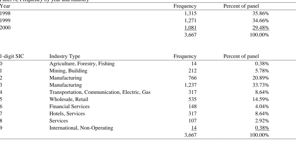
Table 1 summarizes the sample composition by year and industry. Panel A shows 1,315 companies in 1998; 1,271 in 1999; and 1,081 in 2000, for a total of 3,667 firm-year observations, representing 1,362 firms. All but 19 of these firms have simulated book MTRs on Graham’s website during our sample period. Most of our sample firms are manufacturers (SIC2 and SIC3). We perform some tests on a subsample that omits 61 observations from financial service firms (SIC6).
Table 1, Panel B describes how our sample of 1,315 observations in 1998 compares to Compustat’s active and inactive companies’ 1998 assets (data item #6, dollars in millions), sales (#12), pretax income (#170), the absolute value of the
proportion of foreign (#272) to worldwide pretax income (#170), and the total debt (#9+#34) to assets (#6) ratio. To make our comparison, we compute quintiles of the Compustat variables, then determine the percentage of our sample that falls in those ranges. If our sample were perfectly representative of Compustat, one-fifth of the sample would appear in each Compustat quintile. As expected, for variables that indicate size (Assets, Sales) or profitability (Pretax Income), our sample is skewed toward the upper end of the Compustat population. We only compute Foreign Percent for the 466 firms that report nonmissing foreign income (otherwise the first four Compustat quintiles have zero foreign income), and our sample is relatively representative of Compustat’s multinational firms. More of our sample is in the middle of the Leverage distribution than at the tails, suggesting that large multinationals do not often operate with very small or extremely high leverage.
We split the 3,667 years from 1998-2000 into a test sample of 1,833 firm-year observations and a holdout sample of 1,834 firm-firm-year observations. We perform our analysis on the test sample, concluding with a regression to fit public financial statement data to the simulated tax return MTR. In Section 5.2, we use the estimated regression coefficients to predict the tax return MTRs for the holdout sample and compare those MTRs to the benchmark tax return MTRs.
Table 2 presents summary information. Panel A describes various marginal tax rate measures. BookSimMTR is the simulated book marginal tax rate described previously. The mean BookSimMTR is 0.305. The maximum is 0.390, reflecting the narrow “clawback” bracket where the statutory rate is 39 percent before it falls back to the top-bracket statutory rate of 35 percent that applies to most large firms.
We also create categorical marginal tax rate variables commonly used in prior accounting and finance research. Following Plesko (2003), we define NOL as the beginning net operating loss carryfoward (prior year Compustat data item #52) and pretax income as data item #170. We use 35 percent as the top statutory rate to reflect current law.
• If NOL equals zero, then Binary1 equals 0.35. Otherwise, Binary1 equals 0.
• If NOL equals zero and pretax income is nonnegative, then Binary2 equals 0.35. Otherwise, Binary2 equals 0.
• If NOL equals zero and pretax income is nonnegative, then Trichotomous equals 0.35. If NOL is positive and pretax income is negative, then Trichotomous equals zero. Otherwise, Trichotomous equals 0.17.
• If NOL equals zero and pretax income is nonnegative, then PseudoStatutory equals 0.35.11 If NOL is zero and pretax income is negative, then PseudoStatutory equals 0.15. If NOL is positive and pretax income is positive, then PseudoStatutory equals 0.25. Otherwise, PseudoStatutory equals zero.
• If NOL equals zero and pretax income is nonnegative, then Uniform equals 0.35. If NOL is zero and pretax income is negative, then Uniform equals 0.11667. If NOL is positive and pretax income is positive, then Uniform equals 0.23333. Otherwise, Uniform equals zero.
As previously described, we construct prefinancing versions of the variables in which we first add interest expense (Compustat #15) back to pretax income prior to testing whether income is a profit or a loss. As expected, the prefinancing marginal tax rate proxies are slightly larger than each of their post-financing equivalents (e.g., mean Trichotomous is 0.275, but mean Trichotomous (prefinancing) is 0.283). The higher mean for the prefinancing version reflects the fact that some firms have a profit before interest expense but a loss after interest expense.
The tax return simulated marginal tax rate, TaxSimMTR, has a mean of 0.295 and
11
a maximum of 0.390. We also use actual tax return data from 1999-2004 to construct a forward-looking (relative to 1998) categorical variable, FutureSimple, based on realized future taxable income and defined as follows:
• If net income (tax return Line 28) minus NOL and special deductions (Lines 29a and 29b) is less than or equal to zero, then FutureSimple equals zero (but if the firm pays Alternative Minimum Tax (AMT), FutureSimple equals 0.02). If net income minus NOL and special deductions is greater than zero, FutureSimple equals 0.35 (but if the firm pays AMT, FutureSimple equals 0.20).
This definition captures two key features of the tax code: the top statutory rate and the AMT rate (as well as NOL deduction limits for AMT). If a firm does not have a taxable profit, we assign a tax rate of zero unless the firm pays AMT, in which case we assign a tax rate of 2 percent.12 We generally assign the top statutory rate (35 percent) to profitable firms. However, if a profitable firm pays AMT, we assign the 20 percent AMT rate to that firm, assuming that the firm is in a range where preferences and deductions make 20 percent of AMT income greater than 35 percent of regular taxable income.
We calculate FutureSimple rates for 2000 and 2003, and the average discounted tax rate (AvgDiscountedFutureSimple1999-2004) based on a 7.5 percent annual discount rate (the approximate Moody’s corporate bond rate for 1999 to 2004). FutureSimple2000 (0.221), has a higher mean than FutureSimple2003 (0.189), consistent with 2000 being more economically robust.
Table 2, Panel B presents additional summary statistics (expressed in millions of dollars). Our firms are large, with median book assets of $400 million and mean assets
12
Because we do not have all the detail from the AMT form available to us, we cannot be sure that the AMT paid by loss firms arises due to the NOL deduction limitation, but we believe this to be a reasonable assumption.
much larger.13 Median pretax income per books ($27 million) exceeds taxable income ($17 million). Consistent with off-balance-sheet financing or preferences to place external and/or intercompany debt in the U.S., mean tax deductions for interest ($78 million) are higher than worldwide interest expense on the financial statement ($53 million), although median interest amounts are no different ($9 million each for book and tax). These interest expense differences likely contribute to book income exceeding taxable income.
About one-fifth of our sample has losses, as captured by the following dummy variables: worldwide pretax loss (BookLossDummy) 18.2 percent, U.S. pretax loss (USBooklossDummy) 20.1 percent, and taxable loss (Taxloss) 22 percent. Although one-fourth of the sample discloses a net operating loss carryforward on its financial statements, only 7.6 percent has both a current year book loss and an NOL carryforward. A much higher proportion of the tax returns have available NOLs on the tax return (45 percent). Because NOLs acquired from target subsidiaries are difficult to use (due to Internal Revenue Code section 381 and 382 limitations), NOLs that are immaterial for financial statement disclosure can persist on the tax return for many years.
The sample firms have significant multinational activity: 35.3 percent have foreign pretax book income greater than five percent of worldwide pretax book income in absolute value, and 38.5 percent claim a foreign tax credit on the U.S. tax return. Sample firms generally report a current effective tax rate on U.S. income (USETR) below the statutory rate. Mean USETR is only 22.1 percent, and 22.4 percent of our sample firms have an USETR below 10 percent.
13
Book assets from the tax return are larger than consolidated financial statement assets because some firms do not post elimination entries when preparing the Schedule L balance sheet (Boynton et al. 2004).
4.1 Correlation between financial statement and tax return marginal tax rates
Table 3 quantifies the relation between financial statement and tax return MTRs. The first column presents the correlations of TaxSimMTR with BookSimMTR and the other financial statement tax variables. In Panel A (Panel B), all variables are defined on a post-financing (prefinancing) basis. The correlation between TaxSimMTR and BookSimMTR is 67.1 percent in our test sample (Panel A). This correlation is relatively high considering likely consolidation differences and other issues described in Section 3.
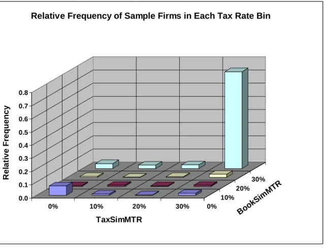
Figure 2 displays the relation between TaxSimMTR and BookSimMTR. Most observations cluster near zero percent and the top statutory rates, reflecting the high correlation between the two tax rates; however, there are only a few clustered observations along the interior diagonal. The main disconnect between BookSimMTR and TaxSimMTR occurs along the back row of Figure 2, where book MTRs are high but tax MTRs vary across the board for these same observations. This reflects that worldwide imputed taxable income based on financial statement data often exceeds taxable income from the U.S. tax return (consistent with the means presented in Table 2, Panel B). We conjecture that another contributing factor is that we exclude discontinued operations and extraordinary items from income in the book simulations but cannot do the same for the tax simulations. Including such items increases the volatility of income (Lipe 1986) and decreases the level of income (Collins et al. 1997), leading to TaxSimMTR having more variation and lower values relative to BookSimMTR.
If we limit the sample to the 45 observations for which the financial statement enterprise likely equals the tax enterprise (per Plesko’s 2003 screens) the correlation
between TaxSimMTR and BookSimMTR increases to 97 percent (untabulated).14 This high correlation arises because Plesko’s screens result in a sample of homogenous firms.
Other common financial statement proxies are not as highly correlated with TaxSimMTR. The worst proxy for our sample is one of the most commonly used in academic research: the net operating loss dummy variable (Binary1, ρ = 0.223). TaxSimMTR is more highly correlated with the financial proxies that assign a top marginal tax rate only if a corporation has neither a current year loss nor an NOL. For example, Binary2 is more highly correlated with TaxSimMTR (ρ= 0.483). However, Binary2 performs worse than the remaining variables, presumably because Binary2 equals zero whenever a firm has an NOL, a loss, or both. Thus, Binary2 can be zero for firms that have a profit, just like Binary1. Trichotomous, PseudoStatutory and Uniform all assign the maximum statutory rate when the corporation has positive income with no NOL, and assign a zero marginal rate when the corporation has both an NOL and a loss. Although they differ slightly in the presence of either an NOL or a loss, but not both, the correlations all improve over Binary1 and Binary2. The correlations of TaxSimMTR with Trichotomous, PseudoStatutory, and Uniform are 0.556, 0.632 and 0.633, respectively.
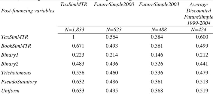
In the second, third and fourth columns of Table 3, Panel A, we compare 1998 values for various tax variables to FutureSimple tax rates that are based on actual future taxable income in 1999 to 2004. TaxSimMTR is highly correlated with all the FutureSimple rates (ρ = 0.564, 0.384, and 0.600), which indicates that ignoring AMT in
14
We replicate the screens imposed by Plesko (2003) in turn. In all cases BookSimMTR is more correlated with TaxSimMTR than are the other financial statement proxies. First, ρ = 78 percent for the 459
observations that have financial statement assets within 0.5 percent of their book assets reported on the tax return, Form 1120, Schedule L. Results are unchanged when we drop one observation that is a domestic subsidiary of another taxpayer and 63 observations for taxpayers that are owned 50 percent or more by another corporation. After we drop another 138 observations for firms that have controlled foreign corporations, ρ = 76 percent for the remaining 257 observations.
the simulation is not a major deficiency. BookSimMTR is also highly correlated with FutureSimple, attenuating concerns that the strong relations between tax return MTRs and the book simulated MTR might be driven by mechanical artifacts (such as using a common discount rate or common historical period to simulate both book and tax MTRs). Of the other variables based on financial statements, Uniform is the most highly correlated with the FutureSimple measures.
Table 3, Panel B repeats the exercise for all the correlations based on prefinancing income. PreIntBookSimMTR is highly correlated (ρ=0.760) with prefinancing TaxSimMTR, more so than correlations for the other prefinancing MTR proxies. BookSimMTR and TaxSimMTR are more highly correlated on a prefinancing basis (in Panel B) than on a post-financing basis (in Panel A), suggesting that book-tax differences in interest expense make it difficult to estimate U.S. taxable income from financial statements (as previously documented in Mills and Newberry 2005). Analogous to the post-financing results, the book net operating loss (Binary1) is the worst proxy for the prefinancing TaxSimMTR (ρ = 0.177).
To construct prefinancing FutureSimple, we add interest deductions (Line 15) to income prior to evaluating loss or profit for the zero and 35 percent rates. PreIntBookSimMTR is highly correlated with each of the prefinancing versions of FutureSimple 2000, FutureSimple 2003 and AvgDiscountedFutureSimple1999-2004 (ρ = 0.428, 0.335 and 0.520, respectively). All the prefinancing FutureSimple variables are more correlated with the PreIntBookSimMTR than with the static prefinancing financial statement proxies (Binary1, Binary2, Trichotomous, PseudoStatutory and Uniform).
simulated book marginal tax rates are reasonable proxies of a firm’s tax return dynamic tax status (Box 3 of Figure 1) because BookSimMTR is more highly correlated with the tax return marginal tax rates than are the other book tax variables.
5. Regressions to explain simulated marginal tax rates
Because a simulated marginal tax rate for the U.S. portion of the enterprise is appropriate for some research questions, we develop algorithms that use publicly available data to “predict” TaxSimMTR. We also develop an algorithm to predict BookSimMTR for situations when it is not available.15 The algorithms include five explanatory variables that address consolidation differences:
TaxSimMTRit = α0 + α1BookSimMTRit+ α2 USBookLossDummyit + α3
LowUSETRDummyit + α4 NOLDummyit + α5 BookLossDummyit + α6
ForeignActivityDummyit + εit,
or
BookSimMTRi = α0 + α1 LowUSETRDummyit + α2 NOLDummyit
+ α3 BookLossDummyit + α4 ForeignActivityDummyit + εit,
where
TaxSimMTR and BookSimMTR are the tax and book simulated tax rates.
USBookLossDummy =1 if Compustat #272 (or, #170 if #272 missing) < 0, zero otherwise.
LowUSETRDummy = 1 if #63/#272 (or, #16/#170 if missing) < 10 percent, zero otherwise.
NOLDummy =1 if #52 > 0, zero otherwise.
BookLossDummy = 1 if nonmissing #170 < 0, zero otherwise.
15
In 2005, there are 6,937 firms on Compusat with nonmissing assets and nonmissing firm identifiers. Graham’s website provides simulated book MTRs for 4,518 of these firms (based on GVKEY matching). That is, there are 2,523 Compustat firms that do not have a 2005 Graham simulated MTR match. These observations are missing either because the firm is new to Compustat and therefore has insufficient historical data to run the simulation (1,408 firms) or otherwise has missing data for one or more of the key input variables in the simulation procedure.
ForeignActivityDummy = 1 if |#273/#170| > 5 percent, zero otherwise.
Two of these variables are specifically related to the U.S. entities. We include U.S. book losses and low U.S. current effective tax rates because our univariate analysis revealed mismatches with high BookSimMTR but near-zero TaxSimMTR (see Figure 2). In the TaxSimMTR specification, we include USBookLossDummy, which indicates a U.S. pretax loss, because the corporation could lose money in its U.S. jurisdiction even if it had worldwide profits. In all the models, we include LowUSETRDummy, an indicator for an average U.S. current effective tax rate below 10 percent. With this variable, we capture the presence of U.S. permanent differences that the simulation ignores and any U.S. temporary differences that vary substantially from the worldwide temporary differences that the simulation already incorporates. To the extent that such U.S.-specific differences decrease U.S. taxable income, TaxSimMTR will be lower than BookSimMTR, leading to negative coefficients on USLossDummy and LowUSETRDummy.
We include ForeignActivityDummy to capture the presence of substantial foreign income, although we make no prediction about its sign. TaxSimMTR could exceed BookSimMTR if foreign losses or intercompany payments make U.S. taxable income higher than worldwide financial statement income or if multinational firms have high TaxSimMTR because of their size. Alternatively, if intercompany payments out of the U.S. exceed payments into the U.S., TaxSimMTR could be lower.
Because we also estimate regressions of TaxSimMTR without BookSimMTR as an explanatory variable, and we estimate BookSimMTR separately, we include NOLDummy and BookLossDummy. We expect the coefficients on these variables to be negative when we estimate TaxSimMTR without BookSimMTR, as well as when we model BookSimMTR
as a dependent variable. We are unsure whether these variables will improve the fit of TaxSimMTR in the specification that includes BookSimMTR.
5.1 Regression results
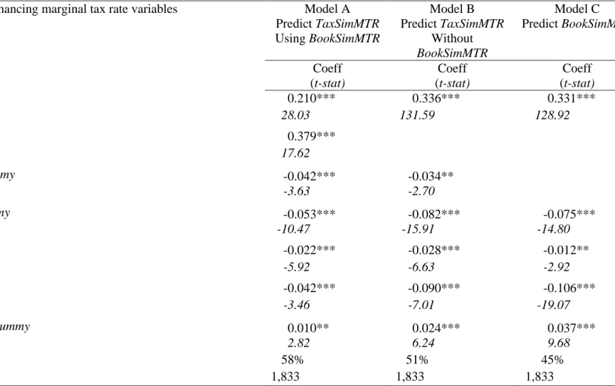
Table 4 presents regression estimates. Panel A uses post-financing marginal tax rates, and Panel B uses prefinancing rates. In Model A, we regress TaxSimMTR on BookSimMTR and additional publicly-available variables. The intercept is 0.21, and the slope coefficient on BookSimMTR is 0.379. By comparison, untabulated univariate regressions of TaxSimMTR on BookSimMTR alone generate an intercept of 0.079 and a slope coefficient of 0.709.The adjusted R2 increases from 45 percent in the untabulated univariate regression to 58 percent in the multivariate regression shown in Panel A.
Model A indicates that negative U.S. pretax income (USBookLossDummy) is significantly associated with a lower TaxSimMTR (coefficient = -0.042, t = -3.63). The negative relation is consistent with U.S. taxable income being negative if U.S. pretax income is negative, even in those cases where a multinational is profitable on a worldwide basis. LowUSETRDummy is strongly negatively associated with TaxSimMTR (coefficient= -0.053, t-statistic = -10.47). We infer that the average current effective tax rate helps to incorporate permanent differences that the simulation cannot easily estimate.16 NOLDummy and BookLossDummy are both negatively related to the dependent variable even though BookSimMTR is already in the regression. TaxSimMTR could be lower for firms that have prior or current book losses because our tax return
16
In untabulated tests, we also include a proxy for corporate tax deductions for exercises of nonqualified stock options, which would decrease taxable income relative to book income. The tax return only requires stock option information starting in 2003. We use the 2003 tax return Schedule M-1 book-tax difference scaled by assets as a proxy for substantial option deductions. This proxy is negatively associated with TaxSimMTR with a t-statistic of -3.00. The backward-looking proxy is undoubtedly extremely noisy, but suggests that better stock option data could improve marginal tax rate simulations.
taxable income includes all sources of loss, including any extraordinary items and discontinued operations that the book forecast of taxable income excludes. Finally, TaxSimMTR is higher in the presence of substantial foreign pretax income. We conjecture that foreign income could proxy for size or repatriations, making U.S. taxable income higher or more consistently profitable than worldwide net income.
In untabulated tests, we find that a wide-scale data-fitting exercise that includes additional Compustat variables does not improve the fit in a stable, informative manner.17 We conclude that the coefficient estimates in the parsimonious Model A of Table 4 can be used to create a reasonable approximation of the simulated tax return MTR for researchers without access to Treasury data.
We also estimate TaxSimMTR without BookSimMTR for cases where BookSimMTR is missing. Model B in Table 4, Panel A shows that the R2 falls to 51 percent, but the overall fit remains strong and the coefficients are similar in magnitude and significance.
Model C shows that the categorical variables are also useful in estimating the BookSimMTR. Researchers who would like to use a simulated book MTR but find it unavailable for certain firms or in certain years can use the coefficients in Model C to estimate the MTR.
Our results (untabulated) are unchanged if we include industry (1-digit SIC) and year controls, and the coefficients on the industry and year dummies are insignificant.
17
We consider 58 additional candidate explanatory variables from the income statement, balance sheet, and statement of cash flow (list of variables is available on request). Using ordinary least squares forward selection, we evaluate each of these variables. Only about ten variables meet the 0.01 significance level. As in the main specification, BookSimMTR and the dummy variables for having negative U.S. pretax book income (book net operating loss carryforward and negative pretax book income) are among these top ten variables; however, the new significant variables are sensitive to the sample (test versus holdout), so we do not pursue this analysis any further.
This suggests that our explanatory variables work reasonably well across industries and our three-year time period. We also estimate our main regression (Table 4, Panel A, Model A) by industry (1-digit SIC) and by year. Only for SIC1 = 6, financial services, is the regression fit substantially different, with the R2 decreasing to 25 percent. Our main results are robust to omitting the 61 firm-year financial services observations.
Panel B of Table 4 presents the results for an analogous set of regressions to estimate prefinancing MTRs. Results are qualitatively the same as in Panel A. Consistent with univariate results from Table 3, TaxSimMTR is more closely associated with BookSimMTR on a prefinancing basis than on a post-financing basis, as indicated by the larger t-statistic in Panel B. As before, researchers who would like to use a simulated prefinancing book MTR but find it unavailable could use the coefficients in Model C to estimate BookSimMTR.
5.2 Analysis using the holdout sample
In Table 5, we report holdout sample correlations between the various tax variables and TaxSimMTR. Because Table 4 presents only the significant variables from among several candidate regression specifications, it is important to determine whether the implications are consistent in the holdout sample.
We compute EST_TaxSimMTR by interacting the regression coefficients estimated in Model A of Table 4 with the applicable variable values for the holdout observations. EST_TaxSimMTR is highly correlated (75.1 percent) with TaxSimMTR in the holdout sample. The 75 percent correlation is equivalent to a univariate regression R2 of 56.25 percent, and recall that the R2 of the predictive regression in Table 3 was 58 percent. Thus, most of the model’s predictive ability carries over to the holdout sample,
indicating that our findings are not driven by data snooping.
The holdout results also shed further light on the univariate relations between the various variables. As in Table 3, BookSimMTR is more highly correlated (65.3 percent) with TaxSimMTR than are the other financial statement proxies (highest correlation equals 63.7 percent).
We replicate these tests on a prefinancing basis in the second column of Table 5. The results are remarkably similar. The prefinancing EST_TaxSimMTR is strongly correlated (ρ = 0.723) with the prefinancing TaxSimMTR in the holdout sample. Like in the test sample, BookSimMTR is more highly correlated on a prefinancing basis with TaxSimMTR than on a post-financing basis. Similarly, the prefinancing BookSimMTR is more highly correlated with prefinancing TaxSimMTR than are the other prefinancing financial statement tax variables.
6. Tax credits and the alternative minimum tax
Our simulation model is based on regular taxable income. Although we simulate income paths and permit loss carrybacks and carryforwards, we ignore tax credits and the alternative minimum tax. In this section, we explain why we believe our simulated rates are reasonable without considering credits and AMT.
Few firms have tax credits that shield a substantial proportion of tax.18 In untabulated tests, 30 percent of the firms in our sample have no tax credits on their tax returns. Further, the firms with the largest proportional credits also have the highest taxable income and the highest foreign tax credits. On average, for firms in the top one-fifth of pretax income, total credits shield 34 percent of tax, and foreign tax credits alone
18
Of the 1,409 observations that report credits, the 95th percentile of credits to total tax is 82 percent and the 99th percentile is 94 percent.
shield 31 percent of tax. Thus, most of the credits for large firms are foreign tax credits, which should not generally reduce the marginal income tax rate on a dollar of U.S. source income.19 The evidence implies that the tax rates that we simulate are likely similar to the marginal tax rates one would obtain if one were to simulate tax rates including the effects of tax credits.
Our simulations also ignore the Alternative Minimum Tax (AMT).20 Untabulated tests using tax return data indicate that firms that pay AMT often claim a NOL deduction (ρ = 0.35). Because our simulation likely assigns a low MTR to firms whose regular income is sheltered by carryforward losses, we have not misstated the MTR materially by ignoring AMT. If a firm pays AMT because of the NOL limitation, the tax rate is effectively two percent. Thus, we do not introduce much error by assigning a zero percent MTR rather than the present value of a two percent temporary AMT rate.21 Recall also that in Table 3, TaxSimMTR (which ignores AMT) is highly correlated with the FutureSimple tax rates that incorporate AMT, again indicating that ignoring AMT in the simulations does not appear to cause significant problems.
7. Which marginal tax rate best captures capital structure tax incentives?
In this section, we test the relative power of prefinancing BookSimMTR and TaxSimMTR to explain capital structure. As in most extant research, we measure capital
19
We acknowledge that foreign tax credits can affect the marginal benefit of an additional dollar of interest deduction (Newberry 1998 and Graham 2003).
20
Graham (1996a) developed his simulated rates shortly after the Tax Reform Act of 1986 created a new AMT adjustment for half of any positive difference between book and taxable income, which was easy to model in the simulation program. This adjustment expired in 1990 and was replaced by an adjustment that is 75 percent of the gap between taxable income and adjusted current earnings (ACE). Because ACE is closer to taxable income and the adjustment can be positive or negative, we do not explicitly account for AMT in our simulations.
21
Also, the AMT is a temporary tax that reverses through a credit when the taxpayer pays regular tax. Both BookSimMTR and TaxSimMTR are significantly, negatively correlated (-44 percent and -45 percent) with the ratio of AMT to tax before credits in untabulated tests. Thus, the simulated MTRs are already low for firms subject to AMT, further confirming the reasonableness of a simulation that ignores AMT.
structure with financial statement debt ratios. The trade-off theory of capital structure predicts that firms with high marginal tax rates should use more debt than firms with low tax rates because the benefit of interest deductions is greater for high tax rate firms.
Despite this straightforward prediction, empirically testing for tax effects is difficult because a spurious relation can exist between the financing decision and many tax variables. Specifically, interest expense is tax deductible, so a firm that finances its operations with debt reduces its taxable income, potentially reducing its expected marginal tax rate. If not properly addressed, this endogeneity of the tax rate can bias an experiment against finding a positive relation between debt ratios and taxes. To avoid this difficulty, we follow Graham et al. (1998) and use a prefinancing measure of the corporate MTR (that is based on taxable income before interest deductions) because it is not endogenously affected by financing decisions. This allows us to regress debt ratios on tax rates without concern of the possibility of a spurious negative relation.
We model leverage (debt to book value of assets in one specification and debt to market value of assets in another) as a function of the prefinancing MTR and control variables:
Leverageit = b0 + b1 PrefinancingMTRit + b2 LagSalesit + b3 LagMarketToBookit
+b4 LagDividendit + b5 LagROAit + b6 LagCollateralit + eit ,
where
Leverage = total debt (Compustat item #9 + #34), scaled by total assets (#6) in one specification, or by market value of assets (total assets minus book equity plus market equity (#6 - #60 + #199*#25)) in a second specification.22
PrefinancingMTR = PreIntBookSimMTR or PreIntTaxSimMTR.
22
Like Mills and Newberry (2005), we do not use leverage ratios from the tax return Schedule L balance sheet because Schedule L is supposed to be a book balance sheet. Further, the assets and liabilities often exceed the worldwide consolidated book amounts, a surprising result that arises from some firms not posting consolidation elimination entries (Boynton et al. 2004).
LagSales = one-year lag of book sales (#12)
LagMarketToBook = the lagged ratio of market value of equity (#199*#25) to book value of equity (#60).
LagDividend = 1 if the lagged dividend yield (#26*100/#199) is positive, zero otherwise. LagROA = lagged return on assets (#18/#6).
LagCollateral = the lagged ratio of receivables and property (#3+#8) to assets (#6). To aid comparison across specifications, we limit the sample to the 1,771 observations that have nonmissing data in all specifications. We expect the simulated book MTR to be better than the simulated U.S. tax return MTR at explaining leverage because, like all Compustat-based research, we define leverage with financial statement data. As discussed above, TaxSimMTR is based on U.S. taxable income, where only domestic corporations owned 80 percent or more are included as affiliates of the U.S. parent, and therefore is defined on a different basis than the dependent variable.
Table 6 shows that PreIntBookSimMTR is strongly positively related to the debt to assets ratio (coeff = 0.294, t = 4.50). The 0.294 coefficient on PreIntBookSimMTR in the debt/assets specification indicates that a one standard deviation increase in the tax variable leads to a debt ratio that is two percentage points higher. For example, if a firm with the sample mean tax rate (0.305) has the sample mean debt ratio (0.26), then if its MTR were one standard deviation (0.102) higher, its debt ratio would change to 0.29 (=0.26+0.294*0.102). We also find that PreIntTaxSimMTR is positively related to the debt to assets ratio (coeff = 0.138, t = 2.02). The explanatory power of the book MTR regression (R2 = 7.3%) exceeds the explanatory power of the tax MTR regression (R2 = 6.4%) based on a Vuong (1989) test (p-value = 0.0496).23
PreIntBookSimMTR is strongly, positively related to the debt to market value ratio (coeff = 0.433, t = 7.73). Likewise, PreIntTaxSimMTR is positively related to the debt to
23
market value ratio (coeff = 0.271, t = 4.59). As above, the R2 (11.4%) of the book MTR regression exceeds the R2 (9.5%) of the tax MTR regression based on a Vuong (1989) test (p-value = 0.0048). The bottom line is that the book simulated MTR appears to best measure worldwide capital structure tax incentives in our sample, leading us to conclude that researchers can continue to use book simulated rates in most capital structure settings.24 This result highlights that tax return data are not the “holy grail” in all experiments, and in fact measuring tax incentives with book data is preferred in some settings (as summarized in Figure 1).
8. Conclusion
Companies likely consider their tax return MTRs when making many decisions but tax returns are not publicly available to researchers investigating those decisions. Therefore, most researchers measure corporate tax incentives using financial statement data. In this paper we access corporate tax return data to simulate a MTR that captures dynamic tax return effects. We compare financial statement tax variables to this (usually unavailable) dynamic tax return MTR to determine which, if any, book MTRs can be used to reliably proxy for the tax return variable when it is unavailable.
We find the simulated financial statement MTR (of Shevlin (1990) and Graham (1996a)) is the best financial statement-based tax rate in terms of most closely approximating the simulated tax return MTR. Thus, our recommendation is that
24
In untabulated tests, we consider two other tax rate variables: 1) The presence of a net operating loss, disclosed either in the financial statements (Compustat #52) or on the tax return (Schedule K); 2) the average tax rate, either worldwide current tax expense divided by pretax income (Compustat #16/#170), or tax after credits divided by net income (line 28 on the tax return), computed for observations with positive numerators and denominators. The alternative tax variables do not perform well. Firms with NOLs have higher leverage, opposite the predicted relation. The current worldwide book effective tax rate is positively related to leverage, as predicted, but the tax return average effective tax rate is negatively related. We conclude that both of these tax variables are poor measures of debt tax incentives. Further details are available on request.
researchers use the simulated book MTR when it is available, assuming that dynamic tax rates are appropriate for a given research setting (see Figure 1). Because the simulated MTR is not always available, we provide coefficients that can be used to create a “predicted” book simulated MTR when it is missing.
We also discuss how different tax rates (book versus tax; dynamic versus static) might be preferred in different experimental settings. For example, we find that financial statement debt ratios, which arguably are the variable under consideration in many capital structure decisions, are highly correlated with the book simulated MTR, consistent with the appropriateness of this tax variable in this setting. In contrast, in other settings, such as transfer-pricing or the issuance of U.S. debt, dynamic tax return MTRs best capture corporate tax incentives, and therefore a simulated tax return MTR would be most appropriate. Because tax return data are often not publicly available, we provide coefficients that can be used to create a “predicted” dynamic tax return MTR.
Finally, as summarized in Figure 1, we also discuss which tax rates might affect decisions in short-term or myopic research settings, such as decisions by retiring executives. Future research is needed to more thoroughly investigate the appropriate tax variable that is or should be used in these short-term settings.
References
Boynton, C., DeFillipes, P., Lisowsky, P., Mills, L., 2004. Consolidation anomalies in form 1120 corporate tax return data. TaxNotes (July 26)
Collins, D., Maydew, E., and Weiss, I., 1997. Changes in the value-relevance of earnings and book values over the past forty years. Journal of Accounting and Economics 24, 39-67.
Contos, G., Rauh, J., and Sorensen, M., 2006. Corporate tax rates, book tax difference, and corporate financial policy. University of Chicago working paper.
Dechow, P., 1994. Accounting earnings and cash flows as measures of firm performance: The role of accounting accruals. Journal of Accounting and Economics 18, 3-42. Desai, M. and Dharmapala, D., 2006. Corporate tax avoidance and high powered
incentives. Journal of Financial Economics, 79:1, 145-179.
Fullerton, D., 1999. Marginal effective tax rate in The Encyclopedia of Taxation and Tax Policy, J. Cordes, R. Ebel, and J. Gravelle, eds (Washington, D.C.: Urban
Institute Press)
Graham, J., 1996a. Debt and the marginal tax rate. Journal of Financial Economics 41, 41-73.
Graham, J., 1996b. Proxies for the corporate marginal tax rate. Journal of Financial Economics 42, 187-221.
Graham, J., 1999. Do personal taxes affect corporate financing decisions? Journal of Public Economics 73, 147-185.
Graham, J., 2003, Taxes and corporate finance: A review, Review of Financial Studies 16, 1074-1128.
Graham, J., Lang, M., Shackelford, D., 2004. Employee stock options, corporate taxes, and debt policy. Journal of Finance 59, 1585-1618.
Graham, J., Lemmon, M., Schallheim, J., 1998. Debt, leases, taxes, and the endogeneity of corporate tax status. Journal of Finance 53, 131-162.
Hanlon, M., 2003. What can we infer about a firm’s taxable income from its financial statements? National Tax Journal 56 (4), 831-863.
Hanlon, M., 2005. The persistence and pricing of earnings, accruals, and cash flows when firms have large book-tax differences. The Accounting Review 80 (1), 137-166.