Dynamic Provisioning: A
Countercyclical Tool for
Loan Loss Reserves
Eliana Balla and Andrew McKenna
T
he methodology to recognize loan losses set forth by the Financial Ac-counting Standards Board (FASB) and the International AcAc-counting Standards Board (IASB) is referred to as the incurred loss model and defined as the identification of inherent losses in a loan or portfolio of loans. Inherent credit losses, under current accounting standards in countries follow-ing FASB and IASB, are event driven and should only be recognized upon an event’s occurrence.1 This has tended to mean that reserves for loan losses ona bank’s balance sheet need to grow significantly during an economic down-turn, a time associated with increased credit impairment and default events. Critics of the incurred loss model have pointed to it as one of the causes of the severity of strain many financial institutions experienced at the onset of the financial crisis of 2007–2009. As rapid provisioning to increase loan loss reserves made headlines, discussions of international regulatory banking reform included the method of dynamic provisioning as a potential alterna-tive to the incurred loss approach (see, for example, Cohen 2009). Dynamic provisioning is a statistical method for loan loss provisioning that relies on historical data for various asset classes to determine the level of provisioning that should occur on a quarterly basis in addition to any provisions that are
The authors would like to thank Teresita Obermann, Jes´us Saurina, and Tricia Squillante for their help in researching the details of the Spanish provisioning system, and Stacy Coleman, Borys Grochulski, Sabrina Pellerin, Mike Riddle, Diane Rose, David Schwartz, and John Walter for their helpful comments. We are also grateful to David Gearhart and Susan Maxey for their research assistance. Any errors are our own. The views expressed in this article are those of the authors and do not necessarily reflect those of the Federal Reserve Bank of Richmond or the Federal Reserve System. The authors can be reached at Eliana.Balla@rich.frb.org and Andrew.McKenna@rich.frb.org.
1 FASB and IASB, March 2009 meeting. Information for Observers. Project: Loan Loss Provisioning.
event driven.2 The primary goal of dynamic provisioning is the incremental
building of reserves during good economic times to be used to absorb losses experienced during economic downturns.
We begin this paper with a discussion of the current approach to loan loss reserves (LLR) in the United States. We argue that, to a social planner who cares both about avoiding bank failures and the efficiency of bank lending, the current accounting and regulatory approach for LLR may be suboptimal on both fronts. First, by taking provisions after the economic downturn has set in, a bank faces higher insolvency risk. When a banker or regulator determines that a bank has inadequate LLR, the bank will have to build the reserves in an unfavorable economic environment. Also, inadequate reserves imply that regulatory capital ratios have been overstated, placing the bank at a higher risk for resolution by the Federal Deposit Insurance Corporation (FDIC). Second, as most banks tend to increase LLR during the economic downturn, the current approach may be procyclical; that is, it may amplify the business cycle. We aim to highlight some of the potential inefficiencies under the incurred loss approach by contrasting it to dynamic provisioning. Dynamic provisioning was instituted in Spain in 2000 in response to some of the same problems we highlight in the United States. We present a conceptual framework to compare loan loss provisioning under the incurred loss framework and dynamic pro-visioning. Then we simulate dynamic provisioning with U.S. data to present an empirical comparison. In the remainder of this section, we offer a brief summary of our main arguments and the conclusions from the simulation exercise.
In accounting terms, the LLR account, also known as the allowance for loan and lease losses (ALLL), is a contra-asset account used to reduce the value of total loans and leases on a bank’s balance sheet by the amount of losses that bank managers anticipate in the most likely future state of the world.3 LLR incorporate both statistical estimates and subjective assessments. Provisioning is the act of building the LLR account through a provision expense item on the income statement. While we present the intuition behind LLR in this section, the Appendix to the paper describes their important accounting features in basic terms.
Interest margin income from loans is a smooth flow whereas a loan default or impairment event causes a lumpy drop in the stock of bank assets. This introduces volatility to banks’ balance sheets. By themselves, a large number
2 Dynamic provisioning is also known as statistical provisioning and countercyclical provisioning.
3 See, for example, Ahmed, Takeda, and Thomas (1999). See Benston and Wall (2005) for a treatment of fair value accounting as it pertains to loan losses. The key to Benston and Wall’s arguments is that if loans could be reported reliably at fair value, where fair value is value in use, there would be no need for a loan loss provision or reserves. But a market for the full transfer of credit risk does not exist and loans cannot be reported reliably at fair value.
of loans may be insufficient to smooth these fluctuations out due to the cor-relation between the risks in the portfolio of bank loans. Some defaults are to be expected in a typical portfolio of bank loans. In order to avoid excess volatility of bank capital levels, banks can build a buffer stock of reserves against expected losses. Intuitively, LLR should serve to absorb expected loan losses while bank capital serves to absorb unexpected losses.4 The key
difference between a conventional economic definition of expected losses and incurred losses is that, unlike expected losses, incurred losses cannot incorpo-rate information from expected future changes into economic variables that affect credit defaults. Incurred losses are entirely based on historical infor-mation.5 If expected losses are greater than the loan loss reserve, regulatory capital ratios overstate the bank capital available to protect against insolvency risk.
To understand the argument that current loan loss accounting standards may have procyclical effects, we have to think about the LLR through the economic cycle. U.S. banking data show that LLR tend to be much lower during good economic times relative to bad economic times. An event-driven approach to LLR does not account for a booming economy resulting in banks relaxing their underwriting standards and taking greater risks.6 Most bad
loans will only reveal themselves in a recession. In that sense, the current approach may magnify the economic boom. By delaying provisioning for loan losses until the economic downturn has set in, the current approach may also magnify the bust. Reserves have to be built at a time when bank funds are otherwise strained, potentially furthering the credit crunch.7 Therefore,
even though banks should want to build “excess” LLR voluntarily during the boom years (it is efficient to do so from their perspective and it would have the benefit of offsetting cyclicality), the accounting guidelines pose a constraint.
4 See Laeven and Majnoni (2003, Appendix A) for a detailed description of the conceptual relationship between LLR, provisions, capital, and earnings.
5 Typically, expected loss is the mean of a loss distribution measured over a one-year horizon (expected loss is loss given default times the probability of default times the exposure at default);
see Davis and Williams (2004). One way to separate the two concepts is by stating that no
expected economic impacts are taken into account in LLR methodology. A bank manager cannot, for example, consider the increases in default risk due to future increases in unemployment.
6 Independently of any LLR effects, stylized facts and a burgeoning literature suggest that
bank lending behavior is procyclical. Many explanations have been presented. The classical
principal-agent problem between shareholders and managers may lead to procyclical banking if
managers’ objectives are related to credit growth. Two of the more recent theories are “herd
behavior” and “institutional memory hypothesis.” Rajan (1994) suggests that credit mistakes are judged more leniently if they are common to the whole industry (herd behavior). Berger and Udell (2003) suggest that, as the time between the current period and the last crisis increases, experienced loan officers retire or genuinely forget about the lending errors of the last crisis and become more likely to make “bad” loans (the institutional memory hypothesis). Our argument here is that LLR effects may add to this otherwise present procyclicality of bank lending.
7 See Hancock and Wilcox (1998) and the sources cited therein for a discussion of the lit-erature on the credit crunch. Also see Eisenbeis (1998) for a critique of Hancock and Wilcox (1998).
“Excess” reserves are associated with managing earnings, which is viewed as undesirable by the accounting profession. Wall and Koch (2000) offer a review of the theoretical and empirical evidence on earnings management via loan loss accounting. The evidence they summarize suggests that banks both have an incentive to and, in general, are using loan loss accounting to manage reported earnings. From the perspective of the accounting profession, using LLR to manage reported earnings is in conflict with the goals of transparency of a bank’s balance sheet as of the date of the financial statement. We take it as a given that the goals and concerns of the accounting standard setters are valid. We simply highlight the resulting tradeoffs.
We illustrate the tradeoffs by pointing to an alternative system of reserv-ing for loan losses—dynamic provisionreserv-ing. Dynamic provisionreserv-ing is, at its core, a deliberate method to build LLR in good economic times to absorb loan losses during an economic downturn, without putting undue pressure on earn-ings and capital. Spanish regulators instituted dynamic provisioning in 2000 explicitly to combat their banking system’s procyclicality.8 In maintaining a focus on the use of historical data in its approach to loan loss provisioning, the Bank of Spain (the regulator of Spanish banks) has been able to adopt dynamic provisioning in compliance with IASB standards. We describe the Spanish method in some detail and present data on Spanish reserves (relative to contemporaneous credit quality) against the United States and other Western European economies in 2006, before the beginning of the crisis. According to these data, the Spanish policy was effective in building relatively higher reserves and thus worthy of further study.
We compare the incurred loss and dynamic provisioning approaches. Through a basic example we illustrate that the key difference is not the level of provisioning but the timing of the provisioning. By taking provisions early when economic conditions are good, banks will avoid using capital in an eco-nomic downturn when it is more expensive, thereby reducing the probability of failure from capital deficiencies. Moreover, a goal of dynamic provision-ing is to ensure that the balance sheet accurately reflects the true value of assets to banks. If income is not reduced to provision for assets that are not collectable, then managers may be pressured to provide greater dividends to investors based on the income that is reported in the period.
As a next step in our analysis, we conduct an empirical simulation to illustrate that a dynamic provisioning framework (akin to the one implemented in Spain) could have allowed for a build-up of reserves during the boom years in the United States. The results demonstrate that the alternate framework would have smoothed bank income through the cycle and provisioning levels
8 In the current provisioning system, outside of Spain, loan loss provisions are generally countercyclical but their effect is thought to be procyclical. We refer to “procyclicality” as the amplification of otherwise normal business fluctuations.
would have been significantly lower during the financial crisis of 2007–2009. Note that, in contrast to accountants, bank regulators would not take issue with LLR resulting in income smoothing because the regulators’ primary concern is the adequacy of the reserves to sustain loan losses.
The remainder of the article proceeds as follows. Section 1 describes current rules for LLR in the United States, as well as the issues confronting the current system, particularly as identified during the financial crisis of 2007– 2009. Section 2 provides a conceptual framework for comparing the incurred loss and the dynamic provisioning approaches to LLR. Section 3 describes the approach as implemented by the Bank of Spain. Section 4 builds a simulation of dynamic provisioning with historical U.S. data. Section 5 concludes.
1. THE CURRENT ACCOUNTING AND REGULATORY
FRAMEWORK FOR LOAN LOSS PROVISIONING IN THE UNITED STATES
Bank regulators view adequate LLR as a “safety and soundness” issue because a deficit in LLR implies that a bank’s capital ratios overstate its ability to absorb unexpected losses. As a result of their important relationship to bank capital and financial reporting transparency, rules governing LLR have been revisited many times by bank regulators and accounting standard setters. Two crucial revision points relate to the new regulatory capital rules in the Basel Capital Accord (signed in 1988) as enacted by the Federal Deposit Insurance Corporation Improvement Act of 1991 (FDICIA)9and the landmark case of
the SunTrust Bank earnings restatement that occured in 1998.10 Changes in capital rules may have reduced bank manager incentives to keep large reserve buffers, while the implementation of accounting rules following the SunTrust case may have made it more difficult to justify building a reserve buffer during good economic times. This section documents current rules that govern LLR, the U.S. data from the last three cycles, and the importance of LLR both for bank solvency and the procyclicality of bank lending.
Incurred Loss Accounting
Provisioning for loan losses in the United States is accounted for under Finan-cial Accounting Standard (FAS) Statement 5, Accounting for Contingencies, and FAS 114, Accounting by Creditors for Impairment of a Loan—an amend-ment of FAS Stateamend-ments 5 and 15. Impaired loans evaluated under FAS 114,
9 See Walter (1991) for extensive coverage of LLR leading to the 1991 changes. Ahmed, Taekda, and Thomas (1999) study how FDICIA (1991) changes affected the relationship between loan loss provisioning, capital, and earnings.
10 See Wall and Koch (2000) for an extensive summary of the theoretical and empirical evidence on bank loan loss accounting and LLR philosophies.
which provides guidance on estimating losses on loans individually evalu-ated, must be valued based on the present value of cash flows discounted at the loan’s effective interest rate, the loan’s observable market price, or the fair value of the loan’s collateral if it is collateral-dependent.11 Loans individually evaluated under FAS 114 that are not found to be impaired are transferred to homogenous groups of loans that share common risk characteristics, which are evaluated under FAS 5. FAS 5 provides for accrual of losses by a charge to the income statement based on estimated losses if two conditions are met: (1) information available prior to the issuance of the financial statements indi-cates that it is probable that an asset has been impaired or a liability has been incurred at the date of the financial statement, and (2) the amount of the loss can be reasonably estimated.12
Both FAS 114 and 5 allow banks to include environmental or qualitative factors in consideration of loan impairment analysis. Examples of these factors include, but are not limited to, underwriting standards, credit concentration, staff experience, local and national economic trends, and business conditions. In addition, FAS 5 allows for the use of loss history in impairment analysis.13
These elements provide bankers with flexibility in determining the level of provisions taken against incurred losses when they are well substantiated by relevant data and/or documentation required by supervisors and accountants. This paper includes illustrative examples to support our explanation of the technical aspects of accounting for loan losses. For consistency, when we refer to identified loan losses, we mean the accounting conditions for taking a provision were met. In practice, banks identify losses by categorizing loans based on their payment status (i.e., current, 30 days past due, 60 days past due, etc.) and the severity of delinquency (which can vary by asset class) and assess whether a provision should be taken on loans they expect to experience a loss, if the loss is probable and estimable.14
The U. S. Data
The adequacy of LLR to cover loan losses is generally measured against the level of non-performing loans (the ratio of the two is known as the coverage ratio), meaning loans that are seriously delinquent by being 90 or more days past due or in non-accrual status. Figure 1 shows LLR and non-performing
11 Financial Accounting Standards Board, Summary of Statement No. 114: Accounting by Creditors for Impairment of a Loan—An amendment of FASB Statements No. 5 and 15 (Issued 5/93).
12 Financial Accounting Standards Board, Summary of Statement No. 5: Accounting for Contingencies (Issued 3/75).
13 SR 06-17: Interagency Policy Statement on the ALLL, December 13, 2006. SR 01-17: Policy Statement on ALLL Methodologies and Documentation for Banks and Savings Institutions, July 2, 2001. SR 99-22: Joint Interagency Letter on the Loan Loss Allowance, July 26, 1999 IPS.
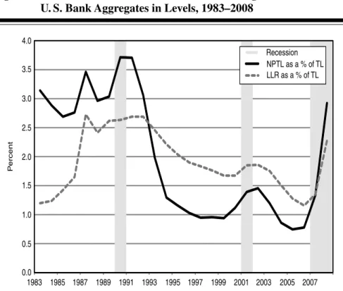
Figure 1 Loan Loss Reserves Versus Non-Performing Loans Ratios: U. S. Bank Aggregates in Levels, 1983–2008
P ercent 4.0 3.5 3.0 2.5 2.0 1.5 1.0 0.5 0.0 1983 1985 1987 1989 1991 1993 1995 1997 1999 2001 2003 2005 2007 Recession NPTL as a % of TL LLR as a % of TL
Notes: LLR = loan loss reserves; NPTL = non-performing total loans; TL = total loans. Source: Call Reports.
loans, both scaled by total loans, between 1983 and 2008. The data come from the Commercial Bank Consolidated Reports of Condition and Income Reports (Call Reports) and they are constructed by combining all U.S. banks into an “aggregate” balance sheet. We show the aggregate level of reserves in the U.S. banking system at any point in time, the aggregate level of non-performing loans, and so on.
Figure 1 depicts the cyclicality of LLR. The first cycle is different from the subsequent two. Reserves are lower than non-performing loans during the banking crisis of the late 1980s and early 1990s. Because of the major regulatory changes that took full effect in 1992, we look more closely at the last two cycles. At the height of the boom, in 2005, we saw some of the lowest reserves relative to total loans on record. Note that this is not surprising given that non-performing loans and reserves move together. At any point between 1992 and 2006, there were more reserves in the system than there were non-performing loans. In 2005, banks had historically high coverage ratios, not
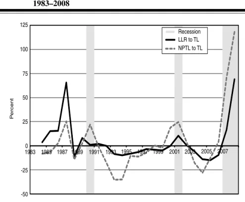
Figure 2 Loan Loss Reserves Versus Non-Performing Loans Ratios: U. S. Bank Aggregates Year Over Year Percentage Change, 1983–2008 P ercent 100 125 75 50 25 0 -25 -50 1983 1985 1987 1989 1991 1993 1995 1997 1999 2001 2003 2005 2007 Recession LLR to TL NPTL to TL
Notes: LLR = loan loss reserves; NPTL = non-performing total loans; TL = total loans. Source: Call Reports.
because reserves were high (indeed they were at a historical low), but because non-performing loans were so low. The period 2006–2008 demonstrated how reserves needed to be built in an economic downturn to keep pace with the rapid deterioration in credit quality. Like credit problems, reserves grow just ahead of a recession and continue to grow after the recession has ended. In the first quarter of 2006, overall U.S. reserves were 1.1 percent of total loans. In the first quarter of 2009, they were built up to 2.7 percent of total loans.
Trends in reserve adjustments against changes in non-performing loans, shown in Figure 2, illustrate that modifications to LLR tend to lag credit prob-lems, and reserves increase more slowly than non-performing loans during economic busts and fall more slowly in booms. Both Figures 1 and 2 indicate that some build-up of reserves relative to non-performing loans existed in the
U.S. banking system but the cushion shrank in the 2000s boom relative to the 1990s boom.15
Loan Loss Provisioning and Bank Solvency
The Basel Accord set current rules for LLR that prescribe the use of impair-ment and estimated loss methodology.16 FDICIA enacted these changes into
law. LLR were no longer counted as a component of Tier 1 capital but were counted toward Tier 2 capital, up to 1.25 percent of the bank’s risk-weighted assets. Laeven and Majnoni (2003) have argued that “. . . from the perspective of compliance with regulatory capital requirements, it became much more effective for U.S. banks to allocate income to retained earnings (entirely in-cluded in Tier 1 capital) than to loan loss reserves (only partially inin-cluded in Tier 2 capital)” (Laeven and Majnoni 2003, 194).
In the new regulatory regime of Basel I, banking regulators remained concerned with the roles that the loan losses and banks’ reserve for losses play in insolvency risk. Comptroller of the Currency John Dugan, the regulator of U.S. national banks, has stated that “. . . banking supervisors love the loan loss reserve. When used as intended, it allows banks to recognize an estimated loss on a loan or portfolio of loans when the loss becomes likely, well before the amount of the loss can be determined with precision and is actually charged off. That means banks can be realistic about recognizing and dealing with credit problems early, when times are good, by building up a large ‘war chest’ of loan loss reserves. Later, when the loan losses crystallize, the fortified reserve can absorb the losses without impairing capital, keeping the bank safe, sound, and able to continue extending credit” (Dugan 2009). But accounting guidelines, as enforced in the late 1990s and 2000s, may have limited the ability of LLR to function in the way summarized by Comptroller Dugan.
In the mid-1990s, the Securities and Exchange Commission (SEC) was increasingly concerned that U.S. banks may be overstating their LLR, po-tentially using this account to manage reported earnings. In 1998, following an SEC inquiry, SunTrust Bank agreed to restate prior years’ financial state-ments, reducing its provisions in each of the years 1994–1996 and resulting in a cumulative reduction of $100 million to its LLR (see Wall and Koch 2000). Analysts of the U.S. banking industry viewed the SunTrust restatement as a permanent strengthening of the existing accounting constraint on a bank’s LLR policy.
15 Note that non-performing loans are only shown as a limited approximation of incurred losses. There is no regulatory guidance that advocates a 100 percent reserve coverage for non-performing loans. Nonetheless, it is a helpful standard simplification to present the data in this way.
16 Basel II: International Convergence of Capital Measurement and Capital Standards: A Revised Framework—Comprehensive Version. http://www.bis.org/publ/bcbs128.htm.
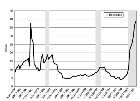
Figure 3 Loan Loss Provisions as a Percentage of Net Operating Revenue: U. S. Bank Aggregates, 1984–2009
Recession P ercent 45 40 35 30 25 20 15 10 5 0 3/31/19846/30/19859/30/198612/31/19873/31/19896/30/19909/30/199112/31/19923/31/19946/30/19959/30/199612/31/19973/31/19996/30/20009/30/200112/31/20023/31/20046/30/20059/30/200612/31/20073/31/2009
Source: Call Reports.
Bankers desire flexibility in recognition of the subjective aspects in deter-mining appropriate reserves. Bank regulators desire flexibility in recognition of the importance of LLR for bank safety and soundness. Accounting stan-dard setters stress the need for transparency and comparability across banks’ financial statements. We take it as a given that the goals of the accounting standard setters and their concern over earnings management are valid. We simply highlight the resulting tradeoffs.
Figure 3 illustrates the importance of provision expense relative to bank income. First, the size of provisions relative to earnings helps us understand their importance to bank managers, accountants, and bank regulators. Sec-ond, the period 2007–2009 illustrates nicely the inverse relationship between earnings and provisions in a recession. Banks had to sharply increase provi-sions in recognition of pending losses, which for many banks more than offset earnings and reduced capital.
Loan Loss Provisioning and Procyclicality
By entering the current economic downturn with low LLR, the banking sector may have unintentionally exacerbated the cycle. In a speech in March 2009, Ben Bernanke, the Chairman of the Board of Governors of the Federal Re-serve stated that there is “considerable uncertainty regarding the appropriate levels of loan loss reserves over the cycle. As a result, further review of ac-counting standards governing. . . loan loss provisioning would be useful, and might result in modifications to the accounting rules that reduce their procycli-cal effects without compromising the goals of disclosure and transparency” (Bernanke 2009).
The cyclicality of loan loss provisioning is well documented with cross-country data. During periods of economic expansion, provisions fall (as a percentage of loans) and, conversely, they rise during downturns. Figure 1 illustrated the cyclicality of loan loss provisioning with U.S. data. As with bank regulatory capital, the concern is that with an approach in which banks have to rapidly raise reserves during bad times, the bad times could get prolonged.17 Laeven and Majnoni (2003) and Bouvatier and Lepetit (2008) document the procyclicality of loan loss provisions with cross-country data. Banks delay provisioning for bad loans until economic downturns have already begun, amplifying the impact of the economic cycle on banks’ income and capital.
Section 1 documented the current framework around LLR in the United States, the U.S. data from the last three cycles, and the importance of LLR both for bank solvency and the procyclicality of bank lending. In response to the recent experience where many banks had to increase their LLR abruptly and drastically, various U.S. and international regulators have expressed the desire to revisit LLR policies. The Financial Stability Forum’s Working Group on Provisioning (2009) has recommended that accounting standard setters give due consideration to alternative approaches to recognizing and measuring loan losses. One approach that has garnered attention is dynamic provisioning.
2. INCURRED LOSS ACCOUNTING VERSUS DYNAMIC
PROVISIONING: A CONCEPTUAL FRAMEWORK
In this section, we discuss and compare dynamic provisioning with the incurred loss methodology using two simplified examples that will set the stage for a more complicated simulation completed in a subsequent section. And, while
17 For simplicity, we are not addressing in this article all the links between LLR and regu-latory capital, nor the similarities between the cyclical effects of LLR and reguregu-latory bank capital. On the latter, we refer the reader to a large literature ranging from Bernanke and Lown (1991) to Peek and Rosengren (1995) to Pennacchi (2005), who use U.S. data to analyze the effects of capital requirements on banks and the economy.
we will review at a high level the technical nuances of accounting, a more detailed discussion of accounting basics is included in the Appendix.
The IASB and the British Bankers Association (BBA) provide more flex-ibility than the FASB for firms to include forward-looking elements based on expectations of total losses over the life of loans, rather than losses already realized, but are still similar to the U.S. standards. The BBA Statement of Recommended Practice on advances indicates specific provisions should be made to cover the difference between the carrying value and the ultimate real-izable value, made when a firm determines that information suggests impair-ment. General provisions18take into account past experience and assumptions
about economic conditions, but are generally small because the Basel Accord of 1988 limits general provisions to 1.25 percent of risk-weighted assets and such provisions are not tax deductible (Mann and Michael 2002).
The IASB, in standard 39, requires assessment at each balance sheet date to determine whether there is objective evidence that an asset or group of assets is impaired—the difference between the asset’s carrying amount and the present value of estimated cash flows discounted at the original interest rate—based on criteria such as the financial condition of the issuer, breach of contract, probability of bankruptcy, and historical pattern of collections of accounts receivable.19
The incurred loss model for accounting for loan losses is divorced from prudential goals of maintaining the safety and soundness of financial insti-tutions in that the FASB and IASB frameworks do not aim to influence the decisions investors make toward a specific objective, such as financial stabil-ity.20 Instead, the goal of financial reporting is to provide financial statement users with the most accurate information about identified losses in the loans and leases portfolio. The dynamic provisioning model, conversely, has as its primary objective the enhancement of the safety and soundness of banks. Its fundamental premise is that when loans are made the probability that default will occur on a loan is greater than zero. In accordance with this philosophy, the dynamic provisioning approach provides a model-based mechanism for a bank to build a stock of provisions in good times so it will not face insolvency due to charge-offs and provisions in bad times. In a simple exercise, presented in Tables 1 and 2, we demonstrate how the application of the incurred loss model would differ from that of dynamic provisioning.21
We will make a number of simplifications to help facilitate an understand-ing of this topic. These assumptions, if not applied, wouldn’t substantively
18 The Bank of Spain refers to statistical provisions as general provisions. See Saurina (2009a).
19 Deloitte: Summaries of International Financial Reporting Standards.
http://www.iasplus.com/standard/ias39.htm.
20 The Financial Crisis Advisory Group. Public Advisory Meeting Agenda, February 13, 2009. 21 The illustration builds on an example provided by Mann and Michael (2002).
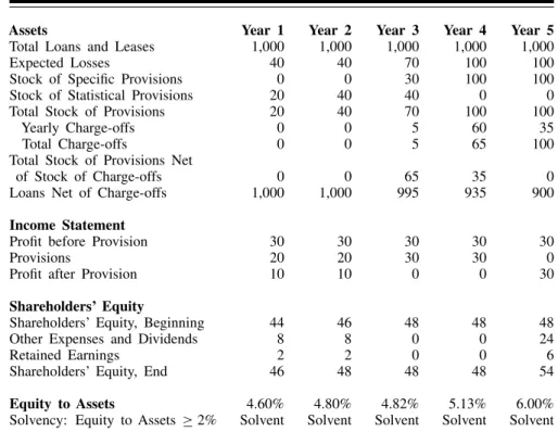
Table 1 Incurred Loss Model
Assets Year 1 Year 2 Year 3 Year 4 Year 5
Total Loans and Leases 1,000 1,000 1,000 1,000 1,000
Expected Losses 40 40 70 100 100
Stock of Specific Provisions 0 0 30 100 100
Yearly Charge-offs 0 0 5 60 35
Total Charge-offs 0 0 5 65 100
Total Stock of Provisions Net
of Stock of Charge-offs 0 0 25 35 0
Loans Net of Charge-offs 1,000 1,000 995 935 900
Income Statement
Profit before Provision 30 30 30 30 30
Specific Provision 0 0 30 70 0
Profit after Provision 30 30 0 −40 30
Shareholders’ Equity
Shareholders Equity, Beginning 44 50 56 56 16
Other Expenses and Dividends 24 24 0 0 24
Retained Earnings 6 6 0 −40 6
Shareholders’ Equity, End 50 56 56 16 22
Equity to Assets 5.00% 5.60% 5.63% 1.71% 2.44%
Solvency: Equity to Assets≥2% Solvent Solvent Solvent Insolvent Solvent
Notes: Expected losses represent bank managers’ expectations for losses over the five-year period in the listed five-year. Specific provisions are those identified as probable and estimable. Yearly charge-offs are those taken in the listed year, while the total is the sum of charge-offs over the five-year period. Equity to assets is shareholders’ equity, end divided by loans net of charge-offs.
change the results of our example, but instead, on average, only reinforce our conclusions. First, the example bank in question will make all its loans in Year 1 and will not grow its portfolio. This prevents us from having to account for changes in bank managers’ preference for varying risks of loans over time as the economic environment changes. Second, we assume that, over the five-year cycle, the bank’s pre-provision profits don’t vary. If we introduced profit declines as conditions worsened, which would likely occur since the bank’s net interest margin (its only source of income in the example) would decline due to charge-offs, the result would be reduced pre-provision profits and the reduction of profit due to provisions would be greater. Third, we assume we know the ex post level of risk in the portfolio of loans. In our example, losses at the end of the five-year cycle will equal 10 percent of the loan portfolio. For illustrative purposes we make the assumption that bank managers believe, based on the bank’s historical loss experience, total ex post losses will equal 4 percent in Year 1 when loans are issued. As a loan approaches maturity in Year 5, managers can, with greater certainty, estimate the true extent of ex
Table 2 Dynamic Provisioning Model
Assets Year 1 Year 2 Year 3 Year 4 Year 5
Total Loans and Leases 1,000 1,000 1,000 1,000 1,000
Expected Losses 40 40 70 100 100
Stock of Specific Provisions 0 0 30 100 100
Stock of Statistical Provisions 20 40 40 0 0
Total Stock of Provisions 20 40 70 100 100
Yearly Charge-offs 0 0 5 60 35
Total Charge-offs 0 0 5 65 100
Total Stock of Provisions Net
of Stock of Charge-offs 0 0 65 35 0
Loans Net of Charge-offs 1,000 1,000 995 935 900
Income Statement
Profit before Provision 30 30 30 30 30
Provisions 20 20 30 30 0
Profit after Provision 10 10 0 0 30
Shareholders’ Equity
Shareholders’ Equity, Beginning 44 46 48 48 48
Other Expenses and Dividends 8 8 0 0 24
Retained Earnings 2 2 0 0 6
Shareholders’ Equity, End 46 48 48 48 54
Equity to Assets 4.60% 4.80% 4.82% 5.13% 6.00%
Solvency: Equity to Assets≥2% Solvent Solvent Solvent Solvent Solvent
Notes: Expected losses represent bank managers’ expectations for losses over the five-year period in the listed five-year. Specific provisions are those identified as probable and estimable. Statistical provisions are those taken under the dynamic provisioning model based on the historical data used to estimate the annual statistical provision. Yearly charge-offs are those taken in the listed year, while the total is the sum of charge-offs over the five-year period. Equity to assets is shareholders’ equity, end divided by loans net of charge-offs.
post losses. To show how provisioning levels are determined over time, we allowed managers’ expectations about expected losses to change in each year to justify provisions each period (the expected losses entry in Tables 1 and 2). Lastly, since the primary intent of dynamic provisioning is to better prepare financial institutions to absorb loan losses, we make assumptions about share-holders’ equity. First, we assume shareshare-holders’ equity is all tangible equity and total loans and leases equal total assets. Accordingly, shareholders’ equity is determined by adding retained earnings, after dividends and expenses, to shareholders’ equity. To determine yearly retained earnings we assume a con-stant ratio of dividend and other expenses equal to 80 percent of after-provision profit. Under current prompt corrective action (PCA) standards used by bank-ing regulators, the Tier I capital ratio, total capital ratio, and leverage ratio are used to determine when banks need to be resolved by the FDIC. In this
Table 3 Capital Guidelines
Leverage Ratio
Well Capitalized 5 percent
Adequately Capitalized 4 percent
Undercapitalized < 4 percent
Significantly Undercapitalized < 3 percent
Critically Undercapitalized < 2 percent
example, since shareholders’ equity most closely resembles tangible equity, we will focus on the leverage ratio, which in the example is equal to equity divided by assets, as the primary measure of solvency. In Year 1 we assume the bank starts with $44 shareholders’ equity and $1,000 total assets, leaving it adequately capitalized at 4.4 percent. The PCA guidelines listed in Table 3 apply to the leverage ratio.
We begin our discussion with the incurred loss model. As previously mentioned, bank managers expect that, given the average risk and performance of loans and leases issued, the banks’total losses will amount to 4 percent of the face value of loans at the end ofYear 5; this is reflected inYear 1, the first column in Tables 1 and 2, listed in the row entitled Expected Losses. However, since data do not exist that support identification of losses—evidence suggesting the 4 percent of losses is probable and estimable—bank managers cannot take provisions until such data exist. In Year 3, the first losses of $30 are identified in the portfolio and managers’ expectation about total losses increases to 7 percent (or $70) based on new data. However, since only $30 in losses have been identified, only a provision of that amount can be taken. Additionally, since the $30 pre-provision profit was wiped out by the provision, the bank’s managers can’t modify other expenses and dividends to increase capital to prepare for the increase in losses. In Year 4, charge-offs increase to $60 for the year and bank managers believe losses will amount to $100, or 10 percent of loans and leases. The bank’s profit of $30 is eliminated by a provision of $70 required by accountants, and a net loss of $40 (shown as negative retained earnings in Table 1) requires the bank to reduce its capital by that amount. When a net loss occurs, banks must use capital to equate assets with liabilities and shareholders’ equity on the balance sheet. The reduction in capital leaves the bank with only $16, resulting in a leverage ratio of 1.71 percent. By PCA standards, this leaves the bank critically undercapitalized and it will be resolved by banking regulators.
Table 2 presents the example bank under dynamic provisioning. Under the dynamic provisioning model, bank managers would take a different approach to provision for loan losses focusing on incrementally building up a fund (referred to as the statistical fund) to protect the bank against losses expected but not yet identified in the loans and leases portfolio. The model driving
the building process for the statistical fund would rely on historical default data for the types of loans and leases issued by the bank rather than models estimating expected losses; this is an important distinction between the dy-namic provisioning approach and a strict expected loss approach. In Year 1, when loans and leases of $1,000 were made, bank managers expected a total of 4 percent of the loans and leases portfolio to default based on its historical data, as reflected in the stock of statistical provisions built. Accordingly, the managers establish a plan to build a fund for the bank to absorb those losses over a two-year period. In Years 1 and 2 the bank provisions $20 to reach the $40 fund desired. This has the effect of reducing profits in those years to $10 instead of $30, which in turn reduces the amount of other expenses and dividends the bank’s managers have and the amount of retained earnings available to build capital. However, since the fund is capital set aside to absorb losses the bank is anticipating based on historical data, the Year 2 capital ratio including the fund is 8.8 percent, compared to 5.6 percent under the incurred loss model in the same year. In Year 3, charge-offs increase to 0.5 percent and the bank’s managers modify their expectation of total losses expected on the loans and leases portfolio to 7.0 percent.
As with the incurred loss model, the $30 identified in specific provisions would also be taken under the dynamic provisioning model. Bank managers, in segmenting specific from statistical provisions, are not only preparing for losses they expect to incur at some point over the life of the loan, but they are also signaling to users of financial statements the difference between the ex-pectation for losses as suggested by the historical data on defaults for the assets held and those actually identified in the portfolio as probable and estimable. The combined fund of $40 and the specific provision of $30 allow the bank to have total provisions equal to $70, preparing the bank to fully absorb the ex-pected losses. And while this reduces profit to $0, the bank’s solvency is well protected. In Year 4, charge-offs increase sharply to $60 and the bank’s man-agers expect losses to increase to $100. Bank manman-agers shift the $40 statistical fund to specific provisions and add $30. After annual charge-offs of $60, the bank has $35 remaining at the end of Year 4 in its stock of provisions to absorb the remaining $35 in identified losses. Again, the bank’s provisioning reduces its profit to $0, but in a difficult economic environment when bank losses are sharply increasing, dividends are being halted throughout the industry and the bank’s managers are actively attempting to reduce expenses, the primary con-cern is solvency. The bank under the incurred loss model becomes insolvent in Year 4, while the bank under the dynamic provisioning model is actually able to increase its leverage ratio, although due to a reduction in balance sheet assets from charge-offs. In Year 5, under the assumption of no recoveries, the remaining charge-offs of $35 occur and the stock of provisions is depleted. The remaining loans and leases are paid down and the bank’s leverage ratio increases again.
This basic example illustrates one of the primary points of importance for dynamic provisioning: the key difference is not the level of provisioning but the timing of the provisioning. By taking provisions early when economic conditions are good, banks may be able to avoid using their capital in an eco-nomic downturn when it is more expensive, thereby reducing the probability of failure from capital deficiencies. Moreover, an objective of dynamic pro-visioning is to ensure that the balance sheet accurately reflects the true value of assets to banks. If income is not reduced to provision for assets that are not collectable, then managers may be pressured to provide greater dividends to investors based on the income that is reported in the period.
3. DYNAMIC PROVISIONING AND THE SPANISH EXPERIENCE
In the wake of the financial crisis of 2007–2009, as various banking poli-cymakers revisit loan loss provisioning rules, there have been calls to study the Spanish experience. The Spanish provisioning system has been credited by most market observers as positioning its banks to avoid the strain that their international peers experienced in 2007. This section reviews the his-torical developments that led to Spain’s adoption of dynamic provisioning. Subsequently, we provide methodological details of the original dynamic pro-visioning approach implemented in 2000 and the modifications made in 2004. Lastly, we briefly discuss the position of Spanish banks at the end of 2006, just prior to the onset of the financial crisis, which will allow readers to gauge the efficacy of the policy; 2006 is the year of emphasis for our analysis because the primary intent of dynamic provisioning is to prepare banks to absorb losses, which, if effective, should have been accomplished by year’s end in 2006.
Why is Spain a Relevant Example?
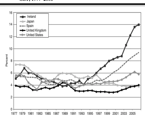
Spain makes for an interesting case in reference to an international financial crisis precipitated by a widespread housing boom.22 Spain’s housing sector boom greatly outpaced the United States’, Japan’s, and the United Kingdom’s, as seen in Figure 4. Spanish loan loss provisions historically demonstrated high procyclicality with the business cycle. From 1991–1999, Spain’s corre-lation between loan loss provisioning levels and GDP was−0.97, the highest in the Organisation for Economic Co-operation and Development (OECD). Similarly, in 1999, Spain had the lowest level of loan loss provisions (to total loans) of any OECD country (Saurina 2009a). In response to pronounced procyclicality, the Bank of Spain in 2000 implemented a countercyclical
22 For a discussion of the housing boom in Spain, see Garcia-Herrero and Fern´andez de Lis (2008).
Figure 4 Gross Fixed Capital Formation in Housing as a Percentage of GDP, 1977–2006 P ercent 16 14 12 10 8 6 4 2 0 Ireland Japan Spain United Kingdom United States 1977 1979 1981 1983 1985 1987 1989 1991 1993 1995 1997 1999 2001 2003 2005
Source: OECD data.
method of loan loss provisioning that allowed banks to build a reserve in good times to cover losses in bad times.23,24
The Original Model
In 1989, the Bank of Spain was authorized to establish the accounting practices of the banks it supervises, helping to resolve the conflict between the objectives of accountants and regulators over issues such as loan loss pro-visioning. The Bank of Spain has historically viewed loan loss provisioning as a necessary policy to accomplish its goals of prudential supervision. In a
23 Subsequent to the Asian Financial Crisis, many emerging Asian economies instituted loan loss provisioning policies (some used discretionary measures) that increased provisioning in good times, leaving the banking system well prepared to absorb losses associated with an economic downturn. For a detailed description of these measures, see Angklomkliew, George, and Packer (2009).
Table 4 Risk Categories Under Standard Approach to Statistical Provisioning: The 2000 Methodology
Category Description
Without Risk (0.0%) Risks involving the public sector
Low Risk (0.1%) Mortgages with outstanding risk below 80 percent of the
property value, as well as risks with firms whose long-term debts are rated at least “A”
Medium-Low Risk (0.4%) Financial leases and other collateralized risks (different
from the former in point 2)
Medium Risk (0.6%) Risks not mentioned in other points
Medium-High Risk (1.0%) Personal credits to financial purchases of durable consumer
goods
High Risk (1.5%) Credit card balances, current account overdrafts, and credit
account excesses
regulation adopted in 2000 upon a foundation set out in Circular 4/1991, the Bank of Spain instituted dynamic provisioning (Poveta 2000). The Bank of Spain places significant emphasis on the growth years in a credit cycle and, given the enhanced procyclicality recognized in Spain (see Fern´andez de Lis, Pag´es, and Saurina 2000), the goal of statistical provisioning is to compensate for the underpricing of risk that takes place during those years. Statistical pro-visioning intends to anticipate the next economic cycle, although it is not meant to be a pure expected loss model because it is backward-looking (Fern´andez de Lis, Pag´es, and Saurina 2000). The statistical fund, built by quarterly provisions recognized on the income statement, was meant to complement the insolvency fund, but, instead of covering incurred losses, was built from estimates of latent losses on homogenous asset groups.
The regulation established two methods for computing the quarterly sta-tistical provision. Banks can create their own internal model using their own loss experience, provided that the data used spans at least one economic cycle and is verified by the bank supervisor. Conversely, banks can use the standard approach outlined by the Bank of Spain, based on a parameter measuring the risk of institutions’ portfolio of loans and leases. For this analysis, our focus will be on the standard approach for two reasons. First, the majority of insti-tutions in Spain use the standard method and, second, the internal models are not available publicly and therefore cannot be the subject of analysis.
The standard approach was developed on the assumption that asset risk is homogenous. The Bank of Spain, in adopting the statistical provision in July 2000, created six risk categories of coefficients by assets for banks to use to take a quarterly provision. The coefficients, shown in Table 4, are based on historical data of the average net specific provision over the period
1986–1998, meant to reflect one economic cycle in Spain.25 Similar to loan
loss provision methods under International Financial Reporting Standards (IFRS) and generally accepted accounting principles (GAAP), the statisti-cal provision is recognized on the income statement and thus has the effect of reducing profits when the difference between the statistical and specific provision is positive. When the statistical provision is negative it reduces the statistical fund, which cannot be negative, and increases profits. The statistical provision is not a tax-deductible expense. To limit the size of the statistical fund, which is a function of the type of assets a bank holds and the duration of economic growth, the fund was capped at 300 percent of the coefficient times the exposure.
The Current Model
In 2004, the Bank of Spain made several modifications to its approach to the statistical provision to conform to the IFRS guidance adopted by the European Union, becoming compulsory for Spanish banks in 2005.26 The following
equation sets out the new approach: General provisiont = 6 i=1 αiCit + 6 i=1 βi− Specific provisionit Cit Cit.
The new model retains a general risk parameter,α, meant to capture the different risks across homogenous categories of assets. For each asset class,α
is the average estimate of credit impairment in a cyclically neutral year; and, although it is meant to anticipate the next cycle, it is not intended to predict it. Two components of theαparameter—that it is backward-looking and unbiased (cyclically neutral)—are crucial in differentiating the policy from an expected loss approach, which would attempt to gauge the characteristics of the next economic cycle through forecasting methods or incorporating expectations about future economic performance. Rather, the use of cyclically unbiased historical data allows provisions to be taken based on the past experience of assets. This feature removes the potential for conflict between banking regulators and banks because there is no discretion over the expectations of
25 Fern´andez de Lis, Pag´es, and Saurina (2000) indicate that the data incorporate banks’ credit risk measurement and management improvements without specifically providing details.
26 The Spanish experience could be considered unique in that the central bank is also the accounting standard setter for banks. Safety and soundness prudential decisions are not made in an accounting vacuum as illustrated by the need for changes to the Spanish model in 2004. The ongoing debate in many countries sets those who argue that a countercyclical reserve account could be made transparent in financial reporting (and sophisticated investors would differentiate the statistical build-up) against the accounting standard setters’ reluctance to turn bank financial reports into prudential regulatory reports. Any LLR reform would involve compromise between bank regulators and accounting standard setters.
Table 5 Risk Categories Under Standard Approach to Statistical Provisioning: The 2004 Methodology
Category Description
Negligible Risk (α=0%, β=0%) Cash and public sector exposures (both
loans and securities)
Low Risk (α=0.6%, β=0.11%) Mortgages with a loan-to-value ratio
below 80 percent and exposure to
corporations with a rating of “A” or higher
Medium-Low Risk (α=1.5%, β=0.44%) Mortgages with a loan-to-value ratio above
80 percent and other collateralized loans not previously mentioned
Medium Risk (α=1.8%, β=0.65%) Other loans, including corporate exposures
that are non-rated or have a rating below “A” and exposures to small- and medium-size firms
Medium-High Risk (α=2.0%, β=1.1%) Consumer durables financing
High Risk (α=2.5%, β=1.64%) Credit card exposures and overdrafts
economic performance that may lead to over- or underprovisioning. It is also beneficial for investors because it provides transparency of provisioning.
In contrast to the original model, the 2004 approach includes aβparameter that interacts with the specific provision (see Table 5). β is the historical average specific provision for each of the homogenous groups. The interaction betweenβ and the specific provision measures the speed with which non-specific provisions become non-specific for each asset class. Cit represents the
stock of assetiat timet. The limit of the statistical fund was modified to 1.25 times latent exposure.27
Spanish Banks in 2006
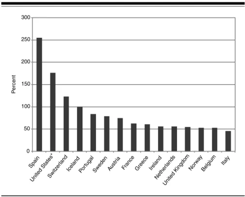
What difference did dynamic provisioning make for Spain?28 In 2006, the
Spanish banking system had by far the highest coverage ratio (the ability of the LLR to cover non-performing loans) among Western European countries at 255 percent. At the same time, the U.S. aggregate coverage ratio was 176 percent.29 Figure 5 shows the coverage ratios for Spain and the United States and also Spain’s European peers as of 2006. To reiterate, 2006 was important
27 The Bank of Spain defines latent loss generally as the probability of default times loss given default. See Saurina (2009a).
28 As part of the Financial Sector Assessment Program, the International Monetary Fund (2006) states that the Central Bank of Spain has pioneered a rigorous provisioning system that enhances the safety and soundness of Spanish banks. While we will briefly discuss the condition of Spanish banks in 2006, see Saurina (2009d) for a more detailed review.
29 The data were obtained from Banco de Espa˜na (2008), U.S. Call Reports, Saurina (2009c) and IMF cited in Catan and House (2008).
Figure 5 Loan Loss Reserves as a Percentage of Non-Performing Assets P ercent 300 250 200 150 100 50 0 Spain United States*Switz
erland
Iceland PortugalSw eden
Austr ia
France Greece Ireland Nether lands United Kingdom Norw ay Belgium Italy
Notes: *The coverage ratio for the United States is the aggregate LLR for all commercial banks as a percentage of the aggregate non-performing loans. It was computed using Call Report data. All other countries’ data come from the International Monetary Fund.
for measurement purposes because the primary intent of dynamic provisioning is the timing of provisions. At the onset of the financial crisis and global recession, dynamic provisioning worked as expected in Spain, allowing large Spanish banks like Santander and BBVA to enter the crisis with substantial reserve cushions relative to non-Spanish peers. Many observers, including G20 Finance Ministers, have singled out the Spanish dynamic provisioning system as a contributor to that banking sector’s soundness entering the financial crisis of 2007–2009. It is beyond the scope of this article to assess what, if any, fraction of banking sector stability in Spain is attributable to dynamic provisioning versus other Spain-specific factors. Additional factors unique to Spain may have a bearing were this policy to be adopted more widely.
4. DYNAMIC PROVISIONING: A SIMULATION WITH U. S. DATA
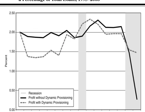
One way to illustrate potential inefficiencies of the current U.S. loan loss provisioning framework is to simulate U.S. bank loan loss provisioning over the last two business cycles under an alternate provisioning framework. This section illustrates that a dynamic provisioning framework (akin to that im-plemented in Spain) could have allowed for a build-up of reserves during the boom years. The results demonstrate that the alternate framework would have smoothed provisions and bank income through the cycle. The severe drop in bank income associated with the actual steep rise in loan loss provisioning during the financial crisis of 2007–2009 would have been substantially re-duced. With positive net income in its place, banks could have increased their capital through internal means and thus reduced the need for assistance from the U.S. government. Note that no precise conclusions can be reached as to the magnitude of these effects from the exercise. Any conclusions based on the simulation are subject to the Lucas Critique in that a change in LLR method-ology is likely to influence bank lending behavior (Lucas 1976). Lending and other related variables would therefore take on values different from those actually observed and used in the simulation. Nonetheless, the simulation is a useful illustration of the relationship between loan loss provisioning and bank income under the two different frameworks.
Using aggregate U.S. data from the year-end quarterly FDIC banking re-ports (key actual data presented in Figure 6),30 we created an example bank.
We have populated the example bank’s financial report with aggregates from a hypothetically consolidated U.S. commercial banking industry so as to ob-serve the interaction of a dynamic provisioning approach with historical U.S. banking data. We apply the 2004 Spanish provisioning methodology to the financials of the example bank so as to display and describe the technical nu-ances of dynamic provisioning. The purpose of this exercise is to demonstrate a well-functioning variant of the policy, that is, how the policy should work, not how it would or would have worked. Accordingly, several simplifying assumptions were required to complete the simulation.
First, we selected representativeαandβ parameters to compute the sta-tistical provision on a yearly basis. We selected 1.8 percent and 0.65 percent, respectively. While an attempt could have been made to approximate the pa-rameters for the example bank, the available banking data does not permit that level of analysis.31 Further, these parameters allowed us to show the results
under a case where the policy is effective and, by examining the results under
30 FDIC Quarterly Banking Profile: 1998–2008
31 The coefficients used in the Spanish standard approach are estimated from a large credit database maintained by the Bank of Spain. No equivalent consolidated credit database exists in the United States as of the publication of this article.
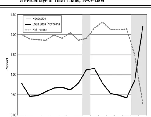
Figure 6 Aggregate U. S. Bank Loan Loss Provisions and Net Income as a Percentage of Total Loans, 1993–2008
2.50 P ercent 2.00 1.50 1.00 0.50 0.00 Recession Loan Loss Provisions Net Income
1993 1994 1995 1996 1997 1998 1999 2000 2001 2002 2003 2004 2005 2006 2007 2008
Source: FDIC data.
this example, readers should be able to also grasp how the results would vary under the case where the parameters were either too high or low.
Second, we had to select a time period for illustrative purposes. The simulation for the example bank begins in 1993 with five years devoted to building the statistical fund. We targeted a build-up of about 2 percent of total loans by 1999 (close to the largest statistical fund possible of 1.25α). Subsequent to 1999, the statistical fund was built using only the statistical provision, shown in line 6 of Table 6 (all line references for the simulation are from Table 6). Line 13 is the actual allowance for loan and lease losses (ALLL),32while line 14 is the ALLL plus the statistical fund, equal to the total
stock of provisions. Line 16, the actual loan loss provision for the year divided by total loans and leases (LLP/TLL), and line 17, the five-year moving
T able 6 Dynamic Pr o visioning Simulation: Example Bank, 1999–2008 (in millions, except TLL) Balance Sheet Accounts 1999 2000 2001 2002 2003 2004 2005 2006 2007 2008 1 TLL, in billions 3,491 3,820 3,889 4,156 4,429 4,904 5,380 5,981 6,626 6,840 2 Actual Rate of Gro wth 7.81% 9.40% 1.83% 6.86% 6.55% 10.74% 9.70% 11.17% 10.80% 3.22% P arameter Scenarios 3 α = 1 . 8% 4 β = 0 . 65% 5 Statistical Fund, Be ginning 69,395 73,238 74,494 62,229 54,873 59,550 67,942 76,329 86,976 82,077 6 Statistical Pro vision 4,411 5,714 976 4,492 4,677 8,392 8,387 10,646 11,249 2,862 7 Statistical Pro vision after Shift 3,843 1,256 0 0 4,677 8,392 8,387 10,646 0 0 8 Amount Needed from Statistical Fund 0 0 12,265 7,356 0000 4,899 86,404 9 Statistical Fund after Shift 69,395 73,238 62,229 54,873 54,873 59,550 67,942 76,329 82,077 0 10 Statistical Fund Limit 78,554 85,940 87,513 93,519 99,649 110,351 121,051 134,567 149,094 153,900 11 Statistical Fund Limit Re v ersal 0000000000 12 Statistical Fund, End 73,238 74,494 62,229 54,873 59,550 67,942 76,329 86,976 82,077 0 13 ALLL 58,770 64,137 72,323 76,999 77,152 70,990 68,688 68,984 89,004 156,152 14 T otal Stock of Pro visions 132,008 138,631 134,552 131,872 136,702 138,932 145,017 155,960 171,081 156,152 Income Statement Accounts 15 LLP 21,814 30,001 43,433 48,196 34,837 26,098 26,610 25,583 57,310 151,244 16 LLP/TLL 0.62% 0.79% 1.12% 1.16% 0.79% 0.53% 0.49% 0.43% 0.86% 2.21% 17 Fi v e-Y ear Mo ving A v erage 0.61% 0.67% 0.78% 0.87% 0.89% 0.88% 0.82% 0.68% 0.62% 0.91% 18 Amount Needed from Statistical Fund 569 4,458 13,242 11,847 0000 16,147 89,266
T able 6 (Continued) Dynamic Pr o visioning Simulation: Example Bank, 1999–2008 (in millions. except TLL) 1999 2000 2001 2002 2003 2004 2005 2006 2007 2008 19 Amount T ak en from Statistical Fund 569 4,458 13,242 11,847 0000 16,147 84,939 20 Ne w Loan Loss Pro vision 21,245 25,543 30,191 36,349 34,837 26,098 26,610 25,583 41,163 66,305 21 Profits W ithout Statistical Pro vision 71,556 71,009 73,967 89,861 102,440 104,172 114,016 128,217 97,630 18,726 22 Changes in Pro visions under Dynamic Pro visioning 3,843 1,256 − 12,265 − 7,356 4,677 8,392 8,387 10,646 − 4,899 − 82,077 23 Profits W ith Statistical Pro vision 67,713 69,753 86,232 97,217 97,763 95,780 105,629 117,571 102,529 100,803
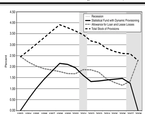
Figure 7 Aggregate U. S. Bank Reserves Compared to Total and
Statistical Reserves as a Percentage of Total Loans, 1993–2008
Recession
Statistical Fund with Dynamic Provisioning Allowance for Loan and Lease Losses Total Stock of Provisions
P ercent 4.50 4.00 3.50 3.00 2.50 2.00 1.50 1.00 0.50 0.00 1993 1994 1995 1996 1997 1998 1999 2000 2001 2002 2003 2004 2005 2006 2007 2008
Source: FDIC data.
average of the same ratio, were used to objectively determine if funds were needed from the statistical fund; the difference between a given year’s LLP/TLL ratio and the five-year moving average determine exactly how much should be drawn from the statistical fund. The statistical provision in a given year was used to cover as much of the amount needed as possible, and then, if necessary, the remaining amount would be taken from the statistical fund; the amount needed from the statistical fund is listed in line 18, while the actual amount taken is listed in line 19. If funds from the statistical provision and statistical fund were used to cover specific provisions, then the loan loss provi-sion in a given year would change. The new loan loss proviprovi-sion reflecting the changes is shown in line 20, and the changes in provisions under the dynamic provisioning simulation, which has an effect on net income, are shown in line 22. The new net income (profit) under the dynamic provisioning simulation is listed in line 23.
The simulation has several interesting results. First, by allowing the bank to use five years to build the fund (during good times from 1993–1998), the
Figure 8 Aggregate U. S. Bank Net Income Compared to Net Income as a Percentage of Total Loans, 1993–2008
Recession
Profit without Dynamic Provisioning Profit with Dynamic Provisioning
P ercent 2.50 2.00 1.50 1.00 0.50 0.00 1993 1994 1995 1996 1997 1998 1999 2000 2001 2002 2003 2004 2005 2006 2007 2008
Source: FDIC data.
example bank was able to build a total stock of provisions, both statistical and specific, of 3.9 percent of total loans. When compared to the actual (U.S. aggregate) total allowance for loan and lease losses of 1.7 percent, the bank is clearly better positioned to withstand losses associated with a recession in 1999. The statistical fund was set to be constrained, if necessary, by the aforementioned limit of 1.25 times the latent losses, which was not reached in the simulation.
The second result to note is the impact of a recession, or increase in loan losses, on the statistical fund. Figure 7 shows total provisions and the statistical fund compared to the actual allowance for loan and lease losses. Both the 2001 and current recessions result in declines in the statistical fund, driving down total provisions, compared to large increases in the actual allowance for loan and lease losses. Since the statistical provision is recorded against the income statement, it reduces profits, as demonstrated in the first example
that contrasted dynamic provisioning to the incurred loss model.33 Figure
8 shows how profits under statistical provisioning compare to actual profits, emphasizing the impact this has on earnings.
The simulation’s primary purpose was to depict the results of dynamic provisioning under one possible scenario with representative parameters se-lected to demonstrate how the policy should work. The sese-lected parameters, combined with the other simplifying assumptions, allow a sizeable fund of statistical provisions to be built in good times and absorb losses in bad times. However, if representative parameters were selected that were too low, higher levels of specific provisioning would have prevented the appropriate fund from being built. Conversely, if higher parameters were selected, then the fund built would have been larger, which could have resulted in inefficiently used capi-tal given the size of realized losses over the time horizon for which the bank provisioned under the policy. This is an important point because the standard approach in the Spanish system is dependent on the parameters estimated by the Bank of Spain.34 The cost of underestimating the risk weights relates to bank-specific solvency, whereas an overestimation of the risk weights is a tax to the bank and could reduce the overall supply of credit.
The simulation illustrates how dynamic provisioning prepared the exam-ple bank to weather the economic downturn while remaining profitable and leaving its capital levels in periods of economic growth accurately stated and allowing managers to further build capital if deemed necessary.
5. CONCLUSIONS
Current accounting guidelines require banks to recognize losses prompted by events that make the losses probable and estimable. But this method may be at odds with the bank regulators’ desire for banks to build a “war chest” of reserves in good times to be depleted in bad times. In 1998, the SEC required SunTrust Bank to restate its LLR by $100 million, reflecting the SEC’s aversion to what it considered to be an overstated reserve. Remarkably, the action taken by the SEC wasn’t long after the banking crises of the 1980s and early 1990s, which, in 1990 alone, resulted in a total provision for loan losses almost twice bank profits (Walter 1991). By the same measure, the financial crisis that began in 2007 was far more severe, resulting in total loan loss provisions greater than eight times bank profits in 2008.35 Following the current episode,
33 Note that both examples treat loan growth rate as independent of reserve rules. Dynamic provisioning is likely to smooth out loan growth expansion and contraction. One could argue that the rules could impose a high enough cost as to result in lower loan volume through the credit cycle.
34 Even banks that use internal models are subject to approval by the Bank of Spain. Pre-sumably, the approval process could involve some reference to the standard risk weights.
Table 7 Aggregate Condition and Income Data: All Commercial Banks, 2008 (in millions)
Assets Liabilities and Capital
Total Loans and Leases $6,839,998 Deposits $8,082,104
Less: Reserve for Loss 156,152 Other Borrowed Funds 2,165,821
Net Loans and Leases 6,683,846 Subordinated Debt 182,987
Securities 1,746,539 All Other Liabilities 724,353
All Other Assets 3,882,529 Equity Capital 1,157,648
Total Assets 12,312,914 Total Liabilities and Capital 12,312,914
Source: FDIC Quarterly Banking Profiles, 2008.
many have called for revisiting the loan loss provisioning method so as to allow for the “war chest” approach and to mitigate the current approach’s procyclical effects.
We compared the incurred loss (as implemented in the United States) and dynamic provisioning (as implemented in Spain) approaches. Through a basic example we illustrated that the key difference is not the aggregate level of provisioning but the timing of the provisioning. We conducted an empirical simulation to illustrate that a dynamic provisioning framework, like the one implemented in Spain, could have allowed for a build-up of reserves during the boom years in the United States. The results demonstrate that the alternate framework would have smoothed bank income through the cycle and the need to provision for loan losses would have been significantly lower during the financial crisis of 2007–2009.
Both in the context of a conceptual framework and through an empirical simulation, we highlighted that dynamic provisioning could mitigate some of the problems associated with the current U.S. system. Even so, it would be premature to advocate the adoption of dynamic provisioning in the United States. We have three reasons for this opinion. First, the distortions embedded in the current U.S. system need to be more fully understood and quantified. Second, although 2006 is a relevant point in time for measuring the efficacy of the Spanish policies, Spanish banking needs to be studied through this cycle and the lessons learned need to be included in potential reform. Third, and most important, the U.S. approach to loan loss reserves should not be reformed independently of other bank capital regulation reform.36
36 To allow for a focus on LLR issues, this article abstracted away from any discussion of broader reform of regulatory capital.
Figure 9 The Balance Sheet
Assets = Liabilities
Assets = Liabilities
Assets = Liabilities
Assets = Liabilities
+
+
+
+
Shareholders' Equity
Contributed
Capital
Contributed
Capital
Contributed
Capital
+
+
+
Retained Earnings
Retained Earnings,
Beginning of Period
Retained Earnings,
Beginning of Period
+
+
Net Income
for Period
Rev. - Exp.
for Period
-Dividends
for Period
Dividends
for Period
Source: Stickney and Weil 2007.APPENDIX: ACCOUNTING FOR LOAN LOSSES
The primary function of banking is to collect depositors’ funds to provide them with transactional support and savings. Banks use depositors’ funds to invest in loans and securities that provide the yields necessary to conduct their operations. As shown in Table 7, as of the second quarter of 2009 loans and securities represented 54.3 and 14.2 percent of total assets for all commercial banks, respectively, while deposits represented 65.6 percent of total liabilities and capital.
As discussed in the subsection entitled “Incurred Loss Accounting,” ac-counting for loan losses is handled under FAS 114 and 5. Under FAS 114, bank managers recognize individually identified losses—that is, losses that managers believe are probable and can be reasonably estimated. FAS 5 pro-vides for assessment of losses of homogeneous groups of loans and, similar to FAS 114, should be probable and estimable.37 In Table 7, listed below
Figure 10 Balance Sheet Accounts
Any Asset Account
Any Liability Account
Any Shareholder's
Equity Account
Beginning
Balance
Beginning
Balance
Beginning
Balance
Increases
+
Debit
Decreases
Credit
Decreases
Debit
Decreases
Debit
Increases
+
Credit
Increases
+
Credit
Ending
Balance
Ending
Balance
Ending
Balance
the total loans and leases, is the reserve for losses, an account that represents the total value of loans and leases that managers expect is probable to not be collected as of the balance sheet data.
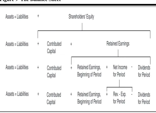
To fully understand the reserve for losses, a brief review of accounting basics is helpful. Figure 9 helps provide a simplified understanding of the balance sheet accounts: assets, liabilities, and shareholders’ equity. The most important concept is the relationship between the income statement accounts (revenue and expenses) and shareholders’ equity. Net income for a firm is computed as revenues for the period minus expenses. Net income flows to shareholders’ equity, dividends are paid, and the remaining funds are