University of Nebraska - Lincoln
DigitalCommons@University of Nebraska - Lincoln
Biological Systems Engineering--Dissertations,
Theses, and Student Research Biological Systems Engineering
Summer 7-18-2019
A Multi-Sensor Phenotyping System: Applications
on Wheat Height Estimation and Soybean Trait
Early Prediction
Wenan Yuan
University of Nebraska - Lincoln, [email protected]
Follow this and additional works at:https://digitalcommons.unl.edu/biosysengdiss
Part of theBioresource and Agricultural Engineering Commons
This Article is brought to you for free and open access by the Biological Systems Engineering at DigitalCommons@University of Nebraska - Lincoln. It has been accepted for inclusion in Biological Systems Engineering--Dissertations, Theses, and Student Research by an authorized administrator of DigitalCommons@University of Nebraska - Lincoln.
Yuan, Wenan, "A Multi-Sensor Phenotyping System: Applications on Wheat Height Estimation and Soybean Trait Early Prediction" (2019).Biological Systems Engineering--Dissertations, Theses, and Student Research. 89.
A MULTI-SENSOR PHENOTYPING SYSTEM: APPLICATIONS ON WHEAT HEIGHT ESTIMATION AND SOYBEAN TRAIT EARLY PREDICTION
by Wenan Yuan
A THESIS
Presented to the Faculty of
The Graduate College at the University of Nebraska In Partial Fulfilment of Requirements
For the Degree of Master of Science
Major: Agricultural and Biological Systems Engineering
Under the Supervision of Professor Yufeng Ge
Lincoln, Nebraska August, 2019
A MULTI-SENSOR PHENOTYPING SYSTEM: APPLICATIONS ON WHEAT HEIGHT ESTIMATION AND SOYBEAN TRAIT EARLY PREDICTION
Wenan Yuan, M.S. University of Nebraska, 2019 Advisor: Yufeng Ge
Phenotyping is an essential aspect for plant breeding research since it is the foundation of the plant selection process. Traditional plant phenotyping methods such as measuring and recording plant traits manually can be inefficient, laborious and prone to error. With the help of modern sensing technologies, high-throughput field phenotyping is becoming popular recently due to its ability of sensing various crop traits
non-destructively with high efficiency. A multi-sensor phenotyping system equipped with red-green-blue (RGB) cameras, radiometers, ultrasonic sensors, spectrometers, a global positioning system (GPS) receiver, a pyranometer, a temperature and relative humidity probe and a light detection and ranging (LiDAR) was first constructed, and a LabVIEW program was developed for sensor controlling and data acquisition. Two studies were conducted focusing on system performance examination and data exploration
respectively. The first study was to compare wheat height measurements from ultrasonic sensor and LiDAR. Canopy heights of 100 wheat plots were estimated five times over the season by the ground phenotyping system, and the results were compared to manual measurements. Overall, LiDAR provided the better estimations with root mean square error (RMSE) of 0.05 m and R2 of 0.97. Ultrasonic sensor did not perform well due to the
wheat height evaluation. The second study was to explore the possibility of early predicting soybean traits through color and texture features of canopy images. Six thousand three hundred and eighty-three RGB images were captured at V4/V5 growth stage over 5667 soybean plots growing at four locations. One hundred and forty color features and 315 gray-level co-occurrence matrix (GLCM)-based texture features were derived from each image. Another two variables were also introduced to account for the location and timing difference between images. Cubist and Random Forests were used for regression and classification modelling respectively. Yield (RMSE=9.82, R2=0.68),
Maturity (RMSE=3.70, R2=0.76) and Seed Size (RMSE=1.63, R2=0.53) were identified
iv ACKNOWLEDGMENTS
I would like to thank my advisor Dr. Yufeng Ge for offering me this great
learning and research opportunity as well as his academic guidance and financial support throughout my master’s program.
I am honored to have Dr. Yufeng Ge, Dr. George Meyer and Dr. P. Stephen Baenziger serving as my committee members.
I would like to thank my colleagues Dr. Geng Bai, Abbas Atefi, Nuwan Kumara Wijewardane, Suresh Thapa, Piyush Pandey, Ujjwol Bhandari,Jiating Li and Arun Narenthiran Veeranampalayam Sivakumar for helping with my difficulties in research and life.
I would like to thank Dr. Geng Bai, Shawn Jenkins, Jiating Li, Madhav Bhatta, Dr. Yeyin Shi, Dr. P. Stephen Baenziger, Dr. George L. Graef and Dr. Yufeng Ge for making my publications possible.
I would like to thank Dr. Geng Bai, Ujjwol Bhandari, Bo Zhang, Yanni Yang, Arena Ezzati See and Hao Zhang for helping me with the field activities.
I would like to thank Scott Minchow for helping me make all the devices used in my projects.
I would like to thank all the instructors of the classes that I have taken at UNL for teaching me the knowledge.
v TABLE OF CONTENTS
ABSTRACT ··· ii
ACKNOWLEDGMENTS ··· iv
TABLE OF CONTENTS ··· v
LIST OF TABLES ··· viii
LIST OF FIGURES ··· ix
LIST OF EQUATIONS ··· xii
CHAPTER 1: INTRODUCTION ··· 1
1.1. Importance of High-Throughput Field Phenotyping ··· 1
1.2. Existing Multi-Sensor Phenotyping Systems ··· 2
1.3. Objectives ··· 10
CHAPTER 2: DEVELOPMENT OF THE MULTI-SENSOR PHENOTYPING SYSTEM ··· 11 2.1. Hardware ··· 11 2.1.1. Sensors ··· 11 2.1.2. Hardware Connection ··· 15 2.2. Software ··· 17 2.2.1. Functions ··· 17 2.2.2. Programming ··· 19
CHAPTER 3: WHEAT HEIGHT ESTIMATION USING ULTRASONIC SENSOR AND LIDAR ··· 22
3.1. Background ··· 22
3.2. Materials and Methods ··· 24
vi
3.2.2. Sensor and Software Setup ··· 26
3.2.3. Height Extraction from LiDAR Point Clouds ··· 28
3.3. Results ··· 34
3.3.1. Raw Point Clouds versus Processed Point Clouds ··· 34
3.3.2. LiDAR Height Estimation Performance by Date, Manual Method and Plot Position ··· 35
3.3.3. Height Estimation Comparison between Ultrasonic Sensor and LiDAR ··· 37
3.4. Discussion ··· 38
3.4.1. Ultrasonic Sensor ··· 38
3.4.2. LiDAR ··· 41
3.5. Conclusions ··· 44
CHAPTER 4: SOYBEAN TRAIT EARLY PREDICTION THROUGH COLOR AND TEXTURE FEATURES OF CANOPY RGB IMAGES ··· 45
4.1. Background ··· 45
4.2. Gray-Level Co-Occurrence Matrix Review ··· 49
4.3. Materials and Methods ··· 53
4.3.1. Data Collection ··· 53
4.3.2. Ground Truths ··· 54
4.3.3. Image Processing ··· 56
4.3.3.1. Pre-processing ··· 56
4.3.3.2. Image Transformations ··· 59
4.3.4. Image Feature Extraction ··· 62
vii 4.3.4.2. Texture Features ··· 62 4.3.5. Data Analysis ··· 64 4.4. Results ··· 66 4.5. Discussion ··· 68 4.5.1. Agronomical Interpretation ··· 68
4.5.2. Limitations of the Study and Directions for Future Studies ··· 72
4.6. Conclusion ··· 73
viii LIST OF TABLES
Table 2.1. Sensor overview of the phenotyping system. ··· 11
Table 3.1. Data collection campaign dates of manual measurement and the ground system for wheat height evaluation. ··· 25
Table 3.2. Optimal RMSE and percentile of raw and processed point clouds at each data collection campaign. ··· 35
Table 3.3. Effects of manual method and plot position on minimum RMSE of processed LiDAR point clouds. ··· 36
Table 4.1. Examples of agriculture-related research utilizing GLCM-based texture features. ··· 49
Table 4.2. Soybean plot and data collection details. ··· 54
Table 4.3. The number of images having the corresponding ground truth available. ··· 56
ix LIST OF FIGURES
Figure 1.1. BreedVision platform and sensor layout (Busemeyer et al. 2013). ··· 3
Figure 1.2. The Maricopa phenotyping system: (a) front view; (b) the sonar proximity sensor; (c) the infrared radiometer; (d) the GPS receiver; (e) the multispectral crop canopy sensor (Andrade-Sanchez et al. 2014). ··· 4
Figure 1.3. Phenomobile and its sensor components (Deery et al. 2014). ··· 5
Figure 1.4. Ladybird robot and its sensor configurations (Underwood et al. 2017). ··· 6
Figure 1.5. Field Scanalyzer and its camera box (Virlet et al. 2017). ··· 8
Figure 1.6. Phenomobile Lite and its sensor components (Jimenez-Berni et al. 2018). ··· 9
Figure 2.1. Flowchart of data communications between sensors and computer of the phenotyping system. ··· 15
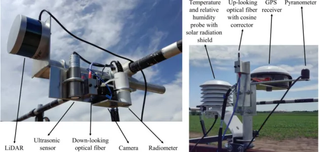
Figure 2.2. Down-looking and up-looking sensor bar of the phenotyping system. ··· 16
Figure 2.3. Inside and outside of the DAQ box of the phenotyping system. ··· 16
Figure 2.4. The assembled phenotyping system. ··· 17
Figure 2.5. Front panel of the LabVIEW program. ··· 18
Figure 2.6. Block diagram of the LabVIEW program. ··· 20
Figure 2.7. Block diagram of the LiDAR subVI. ··· 20
Figure 2.8. Programming logic flowchart of the LabVIEW program. ··· 21
Figure 3.1. Schematic diagram showing the scanning areas of LiDAR and ultrasonic sensors at each measurement. ··· 25
Figure 3.2. The Cartesian coordinate system for LiDAR point cloud at each measurement. ··· 27
Figure 3.3. An example of raw LiDAR point cloud at each measurement. ··· 27
Figure 3.4. The slanting issue of the phenocart in field. ··· 28 Figure 3.5. An example of Y-Z plane rotation correction: (a) Point cloud before rotation; (b) Fit a linear curve to points on Y-Z plane; (c) Rotate points on Y-Z plane by the angle
x
θ; (d) Point cloud after rotation. ··· 29
Figure 3.6. An example of extracting coarse alleyway point clouds: (a) point cloud before rotation; (b) line graph before sorting; (c) line graph after sorting; (d) smoothed line; (e) positions of the four most significant changes; (f) deletion of points beyond the desired range. ··· 30
Figure 3.7. An example of extracting a refined alleyway point cloud: (a) point cloud of ground before cleaning; (b) point cloud kernel density in the Z dimension; (c) first derivative of the kernel density; (d) point cloud of ground after cleaning. ··· 31
Figure 3.8. An example of X-Z plane rotation correction: (a) point cloud of ground before rotation; (b) linear curve fitted to ground points on the X-Z plane; (c) rotation of points on the X-Z plane by the angle φ; (d) point cloud after rotation. ··· 32
Figure 3.9. An example of ground baseline correction: (a) point cloud of ground before shifting; (b) the mean in the Z dimension; (c) points on the X-Z plane shifted by the offset; (d) point cloud after shifting. ··· 33
Figure 3.10. An example of splitting a point cloud: (a) point cloud of ground after rotation and shifting; (b) the mean in the X dimension for each side; (c) point cloud of each plot after splitting. ··· 34
Figure 3.11. RMSE, Bias and R2 of heights extracted at different percentiles from processed LiDAR point clouds over five data collection campaigns. ··· 35
Figure 3.12. Ultrasonic sensor and LiDAR estimated canopy heights versus manually measured canopy heights. ··· 38
Figure 3.13. Two scenarios where ultrasonic sensor estimations disagree with manual measurements. ··· 40
Figure 4.1. Schematic diagram showing the GLCM layout of an image. ··· 52
Figure 4.2. Common scanning directions for generating a GLCM. ··· 52
Figure 4.3. Symmetric GLCM examples of the sample image. ··· 53
Figure 4.4. Normalized GLCM examples of the sample image. ··· 53
Figure 4.5. Flowchart of soybean canopy image pre-processing. ··· 58
Figure 4.6. Examples of colorized transformed images containing different color and texture information. ··· 61
xi Figure 4.7. Prediction results for all soybean traits using all 457 predictor variables. ···· 66 Figure 4.8. Schematic diagram explaining the potential relationships between color and texture information of early-season canopy images and end-season plant
xii LIST OF EQUATIONS Equation 3.1. ··· 26 Equation 3.2. ··· 26 Equation 3.3. ··· 29 Equation 4.1. ··· 53 Equation 4.2. ··· 57 Equation 4.3. ··· 57 Equation 4.4. ··· 57 Equation 4.5. ··· 57 Equation 4.6. ··· 58 Equation 4.7. ··· 62 Equation 4.8. ··· 62 Equation 4.9. ··· 62 Equation 4.10. ··· 62 Equation 4.11. ··· 63 Equation 4.12. ··· 63 Equation 4.13. ··· 63 Equation 4.14. ··· 63 Equation 4.15. ··· 63 Equation 4.16. ··· 63 Equation 4.17. ··· 63 Equation 4.18. ··· 63 Equation 4.19. ··· 64
xiii Equation 4.20. ··· 65 Equation 4.21. ··· 65 Equation 4.22. ··· 65 Equation 4.23. ··· 65 Equation 4.24. ··· 65 Equation 4.25. ··· 65
1 CHAPTER 1
INTRODUCTION 1.1. Importance of High-Throughput Field Phenotyping
Genotype refers to the genetic makeup of an organism, which in a large degree determines the organism’s characteristics. However, genotype itself is not the only factor that would influence gene expression. Environment, or the living conditions of an
organism, also plays a big role in shaping its final appearance. Hence, the term phenotype was created, meaning the set of observable characteristics of an organism resulting from the interaction of its genotype with the environment. In agriculture, plant phenotyping aims to quantitatively describe the morphological, physiological and biochemical properties of a plant (Walter, Liebisch, and Hund 2015), which can have a significant implication for plant breeding in terms of helping understand gene expression under certain environments.
Plant breeding has long been a key method for improving the quality of agricultural products in human history, and one of its fundamentals is plant selection based on plant phenotypes. Since the beginning of domestication to Gregor Mendel’s experiments with pea plant hybridization, plant propagation is more or less dependent on plant phenotyping as newly developed varieties need to be assessed based on certain plant parameters such as yield. The process of quantifying plant traits in a standardized manner is the essence of plant phenotyping, and the quantified plant traits allow breeders to compare different plant varieties and make selections.
2 Modern biotechnologies such as marker-assisted selection and low-cost DNA sequencing have greatly improved the efficiency of genomic research (Behjati and Tarpey 2013), while traditional plant phenotyping in field is not able to keep up with the pace due to its disadvantage of being laborious and inefficient. Humans are typically heavily involved in traditional plant phenotyping activities, such as destructive sampling, visual estimation, or physical measurement of experimental plots. Yet it is challenging to perform those procedures on thousands of plots. Many considered high-throughput field phenotyping as a bottleneck for both conventional and modern plant breeding (Araus et al. 2018; Underwood et al. 2017), and this challenge stands in the way of the next green revolution (Bai et al. 2016), which would be essential for future global food security by 2050 (Ray et al. 2012).
1.2. Existing Multi-Sensor Phenotyping Systems
Diverse approaches for field phenotyping exist. From hand-held devices, fixed in-field sensors, to mobile airborne or ground platforms, each has their unique advantages and limitations (Deery et al. 2014). For example, fixed systems can only monitor limited amount of plots, but they are usually fully automated and can provide measurements in high quality. Airborne platforms such as unmanned aircraft vehicles have limited payload, however they have high data collection efficiency and are not limited by geography. Ground mobiles, on the other hand, can differ from each other greatly in terms of cost, payload, and sensing modules. Generally speaking ground platforms have high payloads and are more flexible in terms of the measuring area, however they tend to be less efficient than airborne platforms.
3 Ground-based multi-sensor phenotyping systems have been gaining popularity in recent years due to their ability of sensing various crop traits non-destructively in a high-throughput fashion, and efforts have been made by researchers and engineers on
developing sophisticated systems in the past. The following are some examples of such systems:
• BreedVision
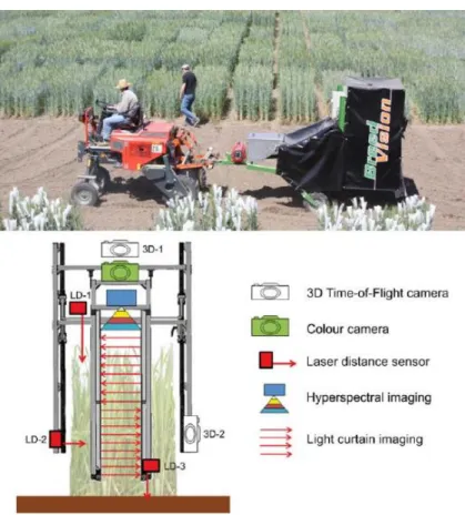
BreedVision was a tractor-pulled phenotyping platform for small grain cereals (Busemeyer et al. 2013). It was equipped with laser distance sensors, light curtains, time-of-flight cameras, a hyperspectral camera, RGB cameras, a GPS receiver and a rotary encoder (Figure 1.1).
4 Based on just a single sensor or the fusion of multiple sensors, the platform can be used for determining simple or complex crop parameters such as plant height, plant moisture content, tiller density and dry biomass yield.
• Maricopa Phenotyping System
A tractor-based multi-sensor system was developed for phenotyping plant dynamic traits and tested in 2011 in Maricopa, Arizona (Andrade-Sanchez et al. 2014). The system carried a GPS receiver and four sets of sensors consisting of a sonar
proximity sensor, an infrared radiometer and a multispectral crop canopy sensor (Figure 1.2).
Figure 1.2. The Maricopa phenotyping system: (a) front view; (b) the sonar proximity sensor; (c) the infrared radiometer; (d) the GPS receiver; (e) the multispectral crop
5 Canopy height, canopy temperature and normalized difference vegetation index (NDVI) of four experimental plots can be measured simultaneously, which all showed differences between cultivars in the study.
• Phenomobile
Deery et al. (2014) reported a buggy for plant phenotyping purposes. The mobile was installed with wheel encoders, a GPS receiver, LiDARs, RGB cameras, a thermal infrared camera, infrared thermometers, a spectrometer and a hyperspectral line scanner camera (Figure 1.3).
Figure 1.3. Phenomobile and its sensor components (Deery et al. 2014).
In the study the possible uses of each sensor component of Phenomobile were explained in details. LiDAR signals are able to show the high contrast betwee soil and vegetation, from whichground cover and possibly plant seedling counts might be evaluated. Aside from basic plant height information, LiDAR’s high resolution data could also be used for estimating advanced canopy structural parameters such as leaf
6 angular distribution. RGB cameras were used for assessing leaf area and volume based on stereo vision algorithm in the study. By moving the mobile slowly, high resolution data could be collected from the hyperspectral camera and the spectrometer, and it was possible to extract the reflectance information from individual plants and distinguish between individual plant organs such as flag leaves and spikes. Spectral vegetation indices could also be calculated to estimate plant parameters such as leaf area index, nutrient contents and water status. Thermal infrared camera was used to assessing canopy temperatures, which could be an indicator for overall canopy transpiration.
• Ladybird
7 Ladybird was an autonomous unmanned ground-vehicle robot for row-crop phenotyping (Underwood et al. 2017), which was also coupled with a data processing framework. The robot is equipped with a GPS receiver and an inertial navigation systems (INS) receiver, forward and rear facing LiDARs, a panospheric camera, a hyperspectral camera, a stereo camera and a thermal camera (Figure 1.4).
Underwood et al. (2017) only reported the application of LiDAR and
hyperspectral camera of the system, and three key crop traits were observed. LiDAR was utilized for crop height measurement since height influences harvest index and lodging risk, and hyperspectral camera was used for NDVI and canopy closure measurements, which are related with chlorophyll and nitrogen concentration, and humidity driven diseases respectively.
• Field Scanalyzer
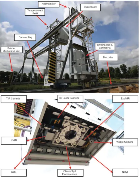
Field Scanalyzer was a fixed site, fully automated robotic phenotyping platform installed at Rothamsted Research, England (Virlet et al. 2017). The system has a camera box, within which multiple sensors were mounted: a visible camera, a thermal infrared camera, 3D laser scanners, a visible and near-infrared camera and an extended visible and near-infrared camera, a NDVI sensor and a chlorophyll fluorescence imager (Figure 1.5).
The actual usage of each sensor component of the system were not described explicitly in the study, however the authors mentioned some potential sensor
applications. RGB camera of the system could be used for monitoring canopy closure, by segmenting plants from soil and calculating the percentage of green pixels of an image. Also it could be used to monitor canopy development overtime and detect and quantify
8 plant organs such as wheat ears. Thermal infrared camera could provide plant
temperature information, which can further be used to assess crop water status. Plant heights could be derived from laser scanner’s point cloud images. Chlorophyll fluorescence imager could help simplify the task of quantifying plant photosynthetic capacity in field at night. The entire spectrum of hyperspectral data could be utilized through multivariate approaches to predict early biotic stress, and plant nitrogen and water content.
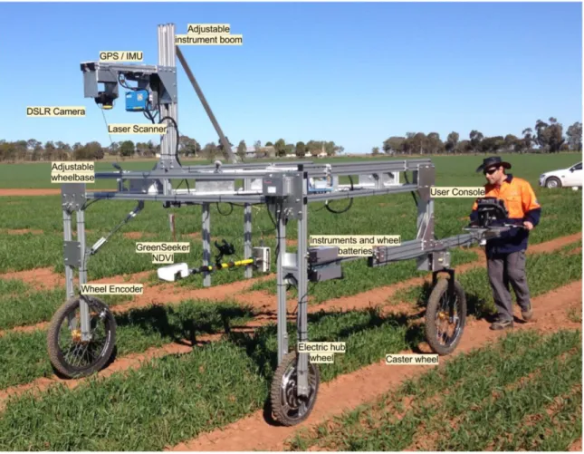
9 • Phenomobile Lite
Phenomobile Lite was a dedicated plant phenotyping mobile with aluminum frame, electric motor and adjustable wheelbase to accommodate for various plot width (Jimenez-Berni et al. 2018). It comprised of a LiDAR, an INS receiver and a GPS receiver and an incremental wheel encoder. The system was also able to integrate other sensors such as active NDVI sensor and digital camera (Figure 1.6). In the study three plant traits were extracted from LiDAR data, namely canopy height, ground cover and above-ground biomass.
10 1.3. Objectives
The primary objective of this thesis was to develop a fully functioning ground-based multi-sensor plant phenotyping system. Two follow-up studies were conducted respectively: the first study was to examine the system’s performance on wheat height estimation; the second study was to explore a new methodology of utilizing RGB images to early predict soybean traits.
11 CHAPTER 2
DEVELOPMENT OF THE MULTI-SENSOR PHENOTYPING SYSTEM 2.1. Hardware
2.1.1. Sensors
Eight types of sensors were selected for the system in order to measure various crop traits and environmental conditions. As an overview, sensor models and
manufacturers, total amounts of sensors employed in the system, sensor input voltage requirements and meanings of sensor measurements were listed in Table 2.1.
Table 2.1. Sensor overview of the phenotyping system.
Sensor Model Manufacturer Amount Voltage Measurement HD Webcam C270 Lausanne, Logitech,
Switzerland Three USB Canopy RGB image SI-131 Infrared
Radiometer
Apogee Instruments, Inc.,
Logan, UT, USA Three 2.5 V Canopy temperature ToughSonic 14 Ultrasonic Sensor Senix Corporation, Hinesburg, VT, USA Three 10 - 30 V Canopy height VLP-16 Puck LiDAR Velodyne LiDAR, Inc., San Jose,
CA, USA One 12 V
Canopy 3D point cloud Flame-S-VIS-NIR Spectrometer Ocean Optics, Inc., Largo, FL,
USA Four USB
Canopy spectral reflectance, incoming radiation spectrum SP-110 Pyranometer Apogee Instruments, Inc.,
Logan, UT, USA One
12 HMP60 Temperature and Relative Humidity Probe Campbell Scientific, Inc.,
Logan, UT, USA One 5 - 28 V
Air temperature, relative humidity AgGPS 162 Receiver Trimble Inc, Sunnyvale, CA, USA One 10 - 16 V Plot location Key sensor specifications and common applications of sensor measurements in field phenotyping were summarized below:
• HD Webcam C270
The webcam uses USB 2.0 for data communication. It has a fixed focus, a 60° diagonal field of view (FOV) and a 1280×960 optical resolution. RGB images contain information regarding plant color and morphology. Estimating plant canopy cover through plant segmentation is a typical usage of RGB images. Vegetation indices based on R, G and B bands can be derived for assessment of plant parameters such as
chlorophyll content (Hunt et al. 2013). Plant 3D canopy structure can also be generated from 2D images using structure from motion (Wilke et al. 2019) or other techniques.
• SI-131 Infrared Radiometer
The radiometer consists of an internal thermistor and a thermopile and it measures temperature based on the Stefan-Boltzmann Law. The thermistor measures the sensor body temperature. It requires a 2.5 V excitation voltage, and typically produces 0 to 2500 mV single-ended signals. The self-powered thermopile measures the infrared radiation emitted or reflected by the target. It has a FOV of 28°, gives approximately -1.1 to 1.1 V differential signals for targets with temperatures ranging from -55 to 55 °C. Along with
13 other parameters such as air temperature, canopy temperature can be used for indicating plant water stress (Jackson, Reginato, and Idso 1977) and assessing plant heat and drought tolerance (Balota et al. 2007).
• ToughSonic 14 Ultrasonic Sensor
The ultrasonic sensor has a total FOV of 14°, and it measures distance from 4 in to 168 in with a resolution of 0.0034 in. The sensor produces 0 to 10 V single-ended signals. Plant height is an important parameter when it comes to plant genotype selection in breeding programs. Besides for plant height, ultrasonic sensors have also been applied for plant biomass estimation (Fricke, Richter, and Wachendorf 2011; Pittman et al. 2015) and weed detection (Andújar, Weis, and Gerhards 2012).
• VLP-16 Puck LiDAR
The LiDAR transfers data via Ethernet. It has 16 near-infrared lasers with a 903 nm wavelength, and it detects distance up to 100 m. The sensor has a vertical FOV of 30° with a resolution of 2°, and a horizontal FOV of 360° with an adjustable resolution between 0.1° and 0.4° (Yuan et al. 2018). Plant 3D point cloud can be used for extracting multiple plant parameters such as height, ground cover, biomass (Jimenez-Berni et al. 2018), leaf area index and plant area density (Deery et al. 2014).
• Flame-S-VIS-NIR Spectrometer
The spectrometer uses USB 2.0 for transferring data. It detects light within the spectral range of 350 to 1000 nm at a 0.1 to 10 nm resolution. The integration time can be set from 1 ms to 65 s. The optical fiber coupled with the spectrometer has a FOV of
14 25.4°. Various vegetation indices such as NDVI can be derived from canopy spectral reflectance and used for assessing vegetation cover, vigor, and growth dynamics (Xue and Su 2017). Due to the limited FOV, spectrometers are not the most practical
instrument for field phenotyping, whereas hyperspectral cameras are gradually becoming the mainstream (Xu, Li, and Paterson 2019).
• SP-110 Pyranometer
The pyranometer has a FOV of 180° and measures solar radiation within the spectral range of 360 to 1120 nm. It generates 0 to 350 mV differential signals. Solar radiation can be used for estimating evapotranspiration and predicting infection risk of fungal diseases, thus is informative for scheduling irrigation and fungicide spraying (López-Lapeña and Pallas-Areny 2018).
• HMP60 Temperature and Relative Humidity Probe
The probe measures temperature from -40 to 60 °C and relative humidity from 0 to 100%. It produces two 0 to 1 V single-ended signals. The difference between air temperature and canopy temperature is typically calculated as an indicator for plant water status as mentioned above. Similarly, along with dry bulb air temperature and net
radiation, wet bulb air temperature can be estimated from relative humidity and crop water stress index can be calculated (Jackson et al. 1981), which is useful for facilitating irrigation scheduling.
• AgGPS 162 Receiver
15 for data communication. The location information of plants helps match phenotypic data with agronomic data, and the unwanted spatial variability in data can be accounted during data analysis (Stroup, Baenziger, and Mulitze 1994). GPS coordinates are also commonly needed for data mapping of certain instruments such as LiDAR.
2.1.2. Hardware Connection
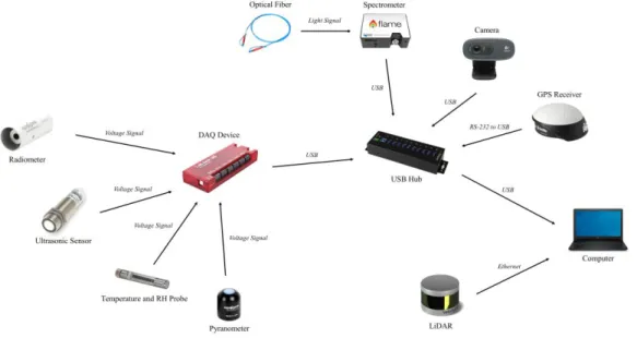
A data acquisition (DAQ) device LabJack U6 with one Mux80 AIN Expansion Board and one CB37 Terminal Board (LabJack Corporation, Lakewood, CO, USA) was used for reading sensor voltage signals. A 10-Port Industrial USB 3.0 Hub
(StarTech.com, Lockbourne, OH) was used for receiving USB signals. Figure 2.1 shows the data communications between different hardware components.
Figure 2.1. Flowchart of data communications between sensors and computer of the phenotyping system.
All hardware components are either installed on “sensor bars” or placed in the “DAQ box”. There are three down-looking sensor bars allowing the system scanning
16 three plots simultaneously, and one up-looking sensor bar for monitoring the environment (Figure 2.2). Except for LiDAR, three down-looking sensor bars have identical sensor arrangements.
Figure 2.2. Down-looking and up-looking sensor bar of the phenotyping system.
Figure 2.3. Inside and outside of the DAQ box of the phenotyping system.
A power supply circuit, the DAQ device, the USB hub and four spectrometers are placed in the DAQ box (Figure 2.3). Sensor USB cables and optical fibers can be directly plugged inside the box, while sensor signal and power wires connect to the box through circular connectors (Figure 2.3).
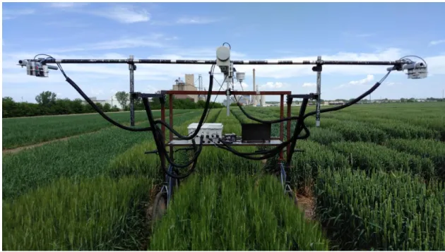
17 The carrier of the phenotyping system, “phenocart”, which consists of two
bicycles, a metal platform and a metal frame, was developed by Bai et al. (2016) (Figure 2.4). Sensor bars can be mounted to the frame through pipefittings, and batteries, DAQ box and computer can be placed on the platform. The phenocart has a clearance of 4 ft, and the wheel spacing between two bicycles is 60 in. The cart can be operated by one or two people using the bicycle handlebars.
Figure 2.4. The assembled phenotyping system. 2.2. Software
2.2.1. Functions
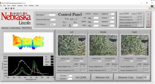
A customized software was developed for sensor controlling and data acquisition using LabVIEW 2016 (National Instruments, Austin, TX, USA) (Figure 2.5). A static measurement style was adopted for the system. Instead of collecting data continuously, sensor outputs were saved only when designated buttons were triggered.
18
Figure 2.5. Front panel of the LabVIEW program. The main functions of the software include the following:
• Allowing users to input Row and Column identification numbers for the plots being scanned if such numbers have been pre-assigned;
• Allowing users to turn on or off data saving for any of the three down-looking sensor bars;
• Allowing users to adjust four camera attributes including brightness, contrast, saturation and sharpness;
• Allowing users to set starting and ending position of LiDAR’s horizontal FOV; • Displaying real-time point cloud of three plots being scanned by LiDAR, and saving point cloud data to csv files when measured;
19 spectra with automatic integration time, and saving spectrum data to csv files when measured;
• Displaying real-time GPS coordinates of the cart, air temperature, relative humidity and total incoming shortwave radiation of the environment, canopy
temperatures and canopy heights estimated from both ultrasonic sensor and LiDAR for three plots being scanned, and saving the readings to one csv file;
• Displaying images of crop canopies captured by the cameras, and saving images as png files.
2.2.2. Programming
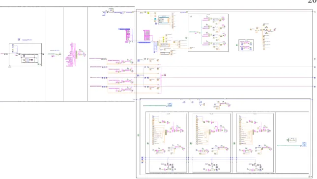
Five major dataflow components existed (Figure 2.6). Built-in LabVIEW virtual instruments (VIs) under “VISA” function palette were used for reading serial port signals from the GPS receiver. Publicly available VIs “LabVIEW_LJUD” were used for reading the voltage signals from the DAQ device’s analog inputs. VIs “Ocean Optics 2000 4000” from Instrument Driver Network of National Instruments were used for calculating the sampling wavelengths of each spectrometer and reading the spectrum signals. Built-in VIs under “NI-IMAQdx” function palette were used for capturing images through the cameras and saving the images. A customized subVI was created for communicating with LiDAR (Figure 2.7), and details can be found in Chapter 3.2.2.
20
Figure 2.6. Block diagram of the LabVIEW program.
Figure 2.7. Block diagram of the LiDAR subVI.
Figure 2.8 shows the basic programming logic of the software. A while loop is used for keeping the program refreshing the sensor readings, which runs once per second. Inside the while loop, a case structure, which examines whether the “Measure” button is triggered or not, is responsible for saving the sensor readings.
21
22 CHAPTER 3
WHEAT HEIGHT ESTIMATION USING ULTRASONIC SENSOR AND LIDAR1
3.1. Background
Plant height is one of the most important parameters for crop selection in breeding programs. For wheat, height is associated with grain yield (Bhatta et al. 2017), lodging (Navabi et al. 2006), biomass (Schirrmann et al. 2016), and resistance to certain disease (Mao et al. 2010). Traditionally plant height is measured manually using a yardstick. This method is labor-intensive and time-consuming when a large number of plants need to be evaluated. In addition, it is prone to error during reading and recording, especially in harsh weather conditions. Alternative but reliable methods for plant height evaluation are needed.
As some of the most common methods for plant height estimation nowadays, ultrasonic sensor and LiDAR are favored over one another because of the unique advantages and disadvantages they possess. Ultrasonic sensor is typically inexpensive and user-friendly, and it has a long history of being utilized in plant height measurement (Fricke et al. 2011). However some of its disadvantages include reduced sensor
accuracies when sensors become farther from objects due to the larger FOV (Sun, Li, and Paterson 2017), sensor’s sensitivity to temperature as sound speed changes with
temperature (Barker et al. 2016), and the susceptibility of sound waves to plant leaf size,
1 This chapter is a portion of a published journal article: Yuan, W., Li, J., Bhatta, M., Shi, Y., Baenziger, P.
S., & Ge, Y. (2018). Wheat Height Estimation Using LiDAR in Comparison to Ultrasonic Sensor and UAS. Sensors, 18(11).
23 angle, and surfaces (Fricke et al. 2011). LiDAR is a relatively new methods for
estimating various plant traits such as height, biomass and ground cover (Jimenez-Berni et al. 2018). LiDAR is considered as a widely-accepted and promising sensor for plant 3D reconstruction because of its high spatial resolution, low beam divergence and versatility regardless of ambient light conditions (Jimenez-Berni et al. 2018; Shi et al. 2015; Underwood et al. 2017). Yet, LiDAR is also costly, and LiDAR data can be voluminous and challenging to process.
Ultrasonic sensor and LiDAR have been both exploited for a wide range of crops in the past. However, ultrasonic sensor was not able to provide consistently accurate height estimations when compared to LiDAR. For example, ultrasonic sensor has been used to estimate the height of cotton (Andrade-Sanchez et al. 2014; Sharma and Ritchie 2015), alfalfa (Pittman et al. 2015), wild blueberry (Chang et al. 2017; Farooque et al. 2013), legume-grass mixture (Fricke et al. 2011; Fricke and Wachendorf 2013),
bermudagrass (Pittman et al. 2015), barley (Barmeier, Mistele, and Schmidhalter 2016) and wheat (Andújar et al. 2012; Pittman et al. 2015; Scotford and Miller 2004), and RMSE from 0.022 to 0.072 m and R2 from 0.44 to 0.90 were observed. On the other
hand, LiDAR has been employed for crops such as cotton (Sun et al. 2017), blueberry (Sun and Li 2016) and wheat (Deery et al. 2014; Friedli et al. 2016; Jimenez-Berni et al. 2018; Madec et al. 2017; Underwood et al. 2017; Virlet et al. 2017), and RMSE from 0.017 to 0.089 m and R2 from 0.86 to 0.99 were obtained.
In existing studies of utilizing terrestrial LiDAR, an experimental field is usually scanned by a LiDAR that moves continuously with a constant speed. For a manned
multi-24 sensor system, this might be problematic since sensors such as cameras often require to be stationary to record high quality data, which can cause difficulties for software programming to harness multiple sensor dataflows simultaneously, as well as actual system operating for maintaining the uniform speed. Moreover, despite all the successes and failures of applying ultrasonic sensor and LiDAR in plant height estimation, a direct comparison between two methods was rarely done in previous research. In this study, we aimed to explore a new methodology of processing LiDAR data in the context of a static measurement style, and compare ultrasonic sensor and LiDAR in terms of their plant height estimation performance.
3.2. Materials and Methods 3.2.1. Experiment Arrangement
The experiment was conducted in 2018 growing season at Agronomy Research Farm in Lincoln, NE, USA (40.86027°N, 96.61502°W). The experimental field contained 100 wheat plots where an augmented design with 10 checks replicated twice was used. The wheat lines consisted of 80 wheat genotypes produced at University of Nebraska– Lincoln, NE, USA. The planting was done at October 20th, 2017, and the plots were
harvested at June 29th, 2018.
Five data collection campaigns occurred over the season. Each time the 100 plots were scanned by the ground phenotyping system (Figure 3.1). The plots were also measured by a yardstick using two methods depending on the growth stage (Table 3.1). At vegetative stages plant height was measured from soil surface to the top of stem, or apical bud (method A). At reproductive stages plant height was measured from soil
25 surface to the top of spike excluding awns (method B). For each plot three measurements were taken and averaged as the reference height of the plot.
Figure 3.1. Schematic diagram showing the scanning areas of LiDAR and ultrasonic sensors at each measurement.
Table 3.1. Data collection campaign dates of manual measurement and the ground system for wheat height evaluation.
Data Collection
Campaign Growth Stage
Manual Ground System
Date Method Date
1st Jointing stage: Feekes 6 May 7th A May 7th
2nd Flag leaf stage: Feekes 8 May 15th A May 15th
3rd Boot stage: Feekes 9 May 23rd B May 23rd
4th Grain filling period: Feekes 10.5.3 May 31st B May 31st
26 3.2.2. Sensor and Software Setup
The measurement rate of ultrasonic sensors was set at 20 Hz. Since only half of the full azimuth range could be possibly useful for our application of scanning crop canopies (Figure 3.1), the LiDAR’s horizontal FOV range was configured as 180°, and a 0.1° horizontal resolution was adopted for higher precision. The sensor was also
configured to report the strongest return for each laser firing.
Voltage signals from ultrasonic sensors were converted to distances in the program through an equation calibrated in lab:
𝐷 = 29.116𝑉 + 11.641, (3.1)
where D is distance in meters and V is sensor signal in volts. Ultrasonic canopy heights
were then calculated as:
𝐻𝑐 = 𝐻𝑠− 𝐷, (3.2)
where Hc is ultrasonic canopy height and Hs is ultrasonic sensor height. Hs was
determined by measuring the distance between the sensors and soil surface before data collection, and LiDAR height was determined in the same way.
The subVI developed for LiDAR was incorporated in the while loop of the main program. The subVI receives data packets from LiDAR through User Datagram Protocol (UDP). Each data packet contains azimuth and distance information of all 16 lasers, and the subVI extracts and converts the information into a 3D Cartesian coordinate system. The origin of the coordinate system is defined as shown in Figure 3.2. After acquiring the XYZ coordinates of the points, the subprogram trims the point cloud in X dimension using a threshold of ±1.5דplot width” (Figure 3.1) to delete points outside the desired
27 range. “Plot width” is defined as the distance between the middles of two adjacent
alleyways, which was 1.524 m in this study. Figure 3.3 is an example of a raw point cloud captured by LiDAR.
Figure 3.2. The Cartesian coordinate system for LiDAR point cloud at each measurement.
28 3.2.3. Height Extraction from LiDAR Point Clouds
One issue that we encountered often in the field was the slant of the phenocart along with the sensor bars due to the unevenness and slope of ground (Figure 3.4). Corresponding LiDAR point clouds thus would show the tilted angle in the Cartesian coordinate system. In order to obtain accurate canopy height estimations from LiDAR, a pre-processing was performed for all raw point clouds to correct for this slanting issue before extracting height information. One assumption for the pre-processing is that the ground slope variation between the three plots within LiDAR’s horizontal FOV can be ignored. LiDAR point clouds were processed using MATLAB R2017a (The MathWorks, Inc., Natick, MA, USA).
Figure 3.4. The slanting issue of the phenocart in field.
It is reasonable to speculate that the points of a point cloud without the slanting issue should be evenly distributed along the Y dimension considering plants with the
29 same genotype should have similar heights. A linear least-squares curve was fitted to the Y-Z plane (Figure 3.5b). The slope of the fitted curve was then converted to an angle θ in
radiance through the relationship:
𝜃 = 𝑎𝑟𝑐𝑡𝑎𝑛 (𝑠𝑙𝑜𝑝𝑒). (3.3)
The point cloud was finally rotated clockwise by the angle θ (Figure 3.5c). The
rotation center could be set at any point, as later the point cloud will be repositioned in the Z dimension.
Figure 3.5. An example of Y-Z plane rotation correction: (a) Point cloud before rotation; (b) Fit a linear curve to points on Y-Z plane; (c) Rotate points on Y-Z plane by the angle
θ; (d) Point cloud after rotation.
A similar procedure was also undertaken for the X-Y plane, which could be skipped as the slanting issue of point clouds on X-Y plane was minimum.
30 As the point distribution along the X-dimension could not be assumed to be even because points were representing plants with different genotypes, linear curve fitting couldn’t be directly applied to the X-Z plane. The method proposed here was to find the rotation angle by finding the average Z value difference between the ground points of two alleyways.
Figure 3.6. An example of extracting coarse alleyway point clouds: (a) point cloud before rotation; (b) line graph before sorting; (c) line graph after sorting; (d) smoothed line; (e)
positions of the four most significant changes; (f) deletion of points beyond the desired range.
The points were first sorted by their X values so that the line graph of the points on the X-Z plane would have a horizontal curve (Figure 3.6c). Then, a moving average filter with a 0.05-m span was applied to smooth the curve (Figure 3.6d). Since the FOV of LiDAR could cover two alleyways, the trend of the curve typically had four abrupt changes in the Z dimension as lasers would scan from the canopy to the ground and back
31 to the canopy twice. After finding the position of the four most significant changes (Figure 3.6e), points with X values smaller than C1, larger than C4, or between C2 and C3
were deleted so that the portion of point cloud that contained two alleyways in the X dimension was extracted (Figure 3.6f).
The point cloud containing two alleyways (Figure 3.6f) was separated into left and right alleyway point clouds using the border of X=0. The non-ground points of two alleyway point clouds were further removed using the procedure explained below.
Figure 3.7. An example of extracting a refined alleyway point cloud: (a) point cloud of ground before cleaning; (b) point cloud kernel density in the Z dimension; (c) first
derivative of the kernel density; (d) point cloud of ground after cleaning. The kernel density in terms of Z values of the alleyway point cloud was first estimated (Figure 3.7b). As the points of ground were typically clustered at the bottom of
32 the Z axis, a dominant peak P1 could be observed from the kernel density graph, which
was also the first peak in the Z axis direction. The first derivative of the kernel density curve was calculated (Figure 3.7c). Assuming ground points follow a normal distribution in the Z dimension, the first peak P2 of the first derivate curve in the Z axis direction
would be the inflection point of the normal distribution, and the distance between P1 and
P2 would be one standard deviation of the distribution. For a normal distribution, the
range μ ± 2σ includes about 95.45% of the values. Here a threshold of μ+2σ on the Z axis was used to separate non-ground points from ground points, where μ is P1 and σ is P1−P2,
and points with Z values larger than the threshold were deleted (Figure 3.7d). After combining refined left and right alleyway point clouds (Figure 3.8a), a linear least-squares curve was fitted to the combined alleyway point cloud on the X-Z plane (Figure 3.8b), and the point cloud with the Y-Z and X-Y plane rotation correction performed (Figure 3.6a) was rotated by the angle φ, which was derived from the slope of
the fitted curve (Figure 3.8c).
Figure 3.8. An example of X-Z plane rotation correction: (a) point cloud of ground before rotation; (b) linear curve fitted to ground points on the X-Z plane; (c) rotation of points
33 The logic of the X-Z plane rotation correction was again executed on the point cloud with the X-Z plane rotation correction already performed (Figure 3.8d) to extract the rotated and refined alleyway point clouds (Figure 3.9a). The average Z value of the alleyway point cloud was calculated (Figure 3.9b), and the Z values of the whole point cloud (Figure 3.9d) were adjusted so that the average Z value of the alleyway point cloud would be located at 0.
Figure 3.9. An example of ground baseline correction: (a) point cloud of ground before shifting; (b) the mean in the Z dimension; (c) points on the X-Z plane shifted by the
offset; (d) point cloud after shifting.
The mean X values S1 and S2 of two alleyway point clouds were calculated
(Figure 3.10b) and used as the border between different plots to split the point cloud (Figure 3.10c). Cumulative Z value percentiles of a point cloud with 0.5 percentage interval from 0 to 100 percent were extracted from each of the three split point clouds. In total there were 200 height values extracted and investigated for each plot.
34
Figure 3.10. An example of splitting a point cloud: (a) point cloud of ground after rotation and shifting; (b) the mean in the X dimension for each side; (c) point cloud of
each plot after splitting. 3.3. Results
3.3.1. Raw Point Clouds versus Processed Point Clouds
To evaluate the effectiveness of LiDAR point cloud pre-processing, plant heights were also extracted from all raw point clouds. With manual measurements being the standard, the minimum RMSE and the corresponding percentile of raw point clouds and processed point clouds at each data collection campaign were compared (Table 3.2).
The point cloud pre-processing consistently improved the precision of LiDAR’s plant height estimation by lowering the minimum RMSE at different data collection campaigns by 12.85 to 44.95%, which confirmed its effectiveness of reducing the influence from uneven ground surface on point clouds.
35 Table 3.2. Optimal RMSE and percentile of raw and processed point clouds at each data
collection campaign.
Data Collection Campaign 1st 2nd 3rd 4th 5th
Raw Point
Clouds Minimum RMSE (m) 0.0462 0.0389 0.0643 0.0467 0.0521 Optimal Percentile 67.5th 85th 99.5th 99th 99.5th
Processed Point Clouds
Minimum RMSE (m) 0.0290 0.0300 0.0354 0.0407 0.0420 Optimal Percentile 60th 91st 99th 99th 99.5th
3.3.2. LiDAR Height Estimation Performance by Date, Manual Method and Plot Position By comparing to manual measurements, RMSE, Bias and R2 of the heights
extracted at each of the 200 percentiles of the processed point clouds across five data collection campaigns were investigated (Figure 3.11).
Figure 3.11. RMSE, Bias and R2 of heights extracted at different percentiles from
processed LiDAR point clouds over five data collection campaigns.
For a point cloud, low percentiles of Z value represent the height of ground, and high percentiles represent the height of vegetation above ground. Since the height of a wheat plot was never measured as the height of the tallest plant, it is easy to understand why RMSE dropped as percentile increased and raised again when percentile approached
36 100 percent. At the percentiles of the minimum RMSE, the average Bias over five data collections was -0.0011 m, which demonstrated LiDAR’s accuracy. The percentiles for maximum R2 fluctuated in between 98 and 99 percent, which did not seem to agree with
the percentiles of minimum RMSE for the first two data collection campaigns (Table 3.2).
Considering the percentile of minimum RMSE could always vary if data were collected at different dates, the optimal percentile at each individual data collection campaign was impractical. Instead of treating all data collection campaigns equally and chose one universal percentile, we classified the 1st and 2nd data collection campaigns as
method A category, and the 3rd, 4th and 5th data collection campaigns as method B
category (Table 3.1) for more precise height estimations. RMSE of method A category, method B category and all category meaning treating all five data collection campaigns as a whole were compared (Table 3.3).
Table 3.3. Effects of manual method and plot position on minimum RMSE of processed LiDAR point clouds.
Category Method A Method B All
Number of Plots 200 300 500
Minimum RMSE (m) 0.0478 0.0398 0.0657
Optimal Percentile 82nd 99th 98th
Sub-category Side Middle Side Middle Side Middle
Number of Plots 140 60 200 100 340 160
Minimum RMSE (m) 0.0436 0.0491 0.0395 0.0327 0.0649 0.0624 Optimal Percentile 77th 89th 99th 99.5th 97th 99th
37 Meanwhile, the effect of plot position on RMSE was investigated as well (Table 3.3). LiDAR had a fixed horizontal resolution, due to which the closer one object was to LiDAR the denser point cloud of that object would be acquired. In our case, the point cloud generated at each measurement included two side plots and one middle plot, and LiDAR was positioned above the middle plot, thus middle plots had denser point clouds than side plots. On average the point clouds of side plots had about 6000 points while the ones of middle plots had about 8000 points.
Based on Table 3.3, manual method affected RMSE substantially as the minimum RMSE of all category was 37.45% and 65.08% higher than the minimum RMSE of method A and B categories respectively, thus it makes more sense to use different optimal percentiles for two method categories for future work. However plot position didn’t seem to affect RMSE in a significant way, with an average RMSE increase of 0.0026 m when plot positions weren’t differentiated in two method categories, hence the effect of plot position can be ignored in the future as the additional RMSE should be minor.
3.3.3. Height Estimation Comparison between Ultrasonic Sensor and LiDAR
Over five data collection campaigns, ultrasonic senor estimated canopy heights and LiDAR estimated canopy heights where 82nd and 99th Z value percentiles of
processed point clouds were chosen for method A and B categories were plotted against manual measurements (Figure 3.12).
38
Figure 3.12. Ultrasonic sensor and LiDAR estimated canopy heights versus manually measured canopy heights.
Among two methods, LiDAR performed much better than ultrasonic sensors. With a large RMSE of 0.34 m and a low R2 of 0.05, ultrasonic sensors tended to
overestimate wheat canopy heights at the 1st data collection campaign and underestimate
heights at the rest data collection campaigns, also it provided some negative readings, which will be discussed in Section 3.4.1. LiDAR provided precise and accurate height estimations throughout the season, with a low RMSE of 0.05 m, a low Bias of -0.02 m and a high R2 of 0.97. In terms of the results, LiDAR can be considered as a reliable plant
height evaluation method. 3.4. Discussion
3.4.1. Ultrasonic Sensor
The poor performance of ultrasonic sensors in this study can be explained by sensor limitations, wheat morphology and our measurement style. Ultrasonic sensor
39 generates sound waves to detect distances. When the sound waves are not reflected straight back to the sensor, due to either sensor orientation or object surface orientation, ultrasonic sensor may not capture the reflected sound waves. In this study the slanting issue of the phenocart could be a cause for that. Also when the surface of an object is not large enough to create strong echoes, ultrasonic sensor may not treat the weak echoes as valid signals. A typical wheat plant has narrow leaves and thin spikes, thus making it hard for ultrasonic sensors to pick up valid signals reflected from wheat. Moreover, because of our static measurement style, for each plot the ultrasonic sensor was only able to sample a small area (about 0.05 m2 assuming one meter distance between sensor and
canopy) to represent the whole plot. Due to within-plot variation, the random error from sampling could not be assessed or corrected, which led to ultrasonic sensors’ low performance. Andújar et al. (2012) also used ultrasonic sensors in a static measurement style to detect weeds in wheat plants, and a low Pearson's correlation of 0.32 between ultrasonic sensor readings and manually measured wheat heights was observed.
The overestimation and underestimation of wheat height by ultrasonic sensors are illustrated in Figure 3.13. For a young wheat plant, clustered leaves with natural
curvature seemed to reflect sound waves effectively, however the reference height was measured as the height of stem top instead of leaf top (method A). As wheat plants grew taller and started to emerge spikes, only the vegetation at the bottom seemed to have sufficient density to reflect strong echoes, which was lower than the manually measured spike tip height (method B).
40
Figure 3.13. Two scenarios where ultrasonic sensor estimations disagree with manual measurements.
Near-zero canopy heights can appear when ultrasonic sensors cannot detect any significant echoes except for those reflected from ground. Moreover, if the phenocart is slanted so that the distance between ultrasonic sensors and ground at a given moment is larger than Hs in Equation 3.2, negative canopy heights will be recorded.
To improve plant height estimation of ultrasonic sensors, a continuous
measurement style—i.e., multiple measurements per plot—is preferred. In a previous study by Scotford and Miller (2004), approximately 180 wheat height measurements from ultrasonic sensor were recorded for each plot, and it was found that the 90% percentile of each data set provided the best wheat height estimation, with the lowest RMSE for a wheat variety of 0.046 m. Pittman et al. (2015) extracted 25 to 30 ultrasonic sensor readings per wheat plot, and found a Pearson’s R of 0.85 compared to manual measurements.
41 obtaining better ultrasonic height estimations. In the context of our manned multi-sensor system, however, the phenocart was often required to stop to capture images. Two issues could occur if a continuous measurement style were adopted for the system: first, due to the highly variable phenocart speed on a field with a rough surface, inconsistent numbers of height measurements could be recorded for different plots; second, a large number of repeated measurements will be taken from the same sampling area when the phenocart is stationary. Both issues can Bias the data and make them troublesome to process. The static measurement style may, therefore, still be preferable for our system, in which case the ultrasonic sensor is not the best method for wheat height estimation.
3.4.2. LiDAR
The LiDAR point cloud pre-processing proposed in this study effectively reduced the influence from the slanting issue of the phenocart on the field. However, when ground is fully covered by vegetation, LiDAR with strongest return mode might not capture enough ground points, and pre-processing of the point cloud could not be undertaken. Due to the beam divergence of the lasers, a single firing of a laser can hit multiple objects resulting in multiple returns, and, typically, LiDAR can be configured to report multiple returns. A suggested solution is to configure LiDAR in multiple return mode since the last return signal has a higher chance of being reflected by soil, so a sufficient amount of ground points might be collected.
For processed point clouds, the minimum RMSE and the corresponding percentile increased as wheat grew taller (Table 3.2). As method B was measuring the tip of wheat spikes while method A was measuring the top of wheat stems, it was expected that the
42 optimal percentiles increased with data collection campaigns. Wind was suspected to be the reason for the increasing RMSE. As wheat plants get taller, wind can cause a larger degree of bending in plants, and LiDAR can capture deformed point clouds due to wind. At the fifth data collection campaign, when the minimum RMSE was the largest, the wind speed on the field was maintained at 8.0 to 8.9 m/s, with gust speeds up to 14.8 m/s.
Generally, extracting plant heights from point clouds can include the following steps: soil level estimation, noisy point removal, rasterization of the point cloud, and percentile selection. Similar to the purpose of our ground baseline correction (Yuan et al. 2018), most studies removed the effect of uneven soil levels by subtracting the
corresponding soil height from vegetation points. The peak of a point cloud’s Z value histogram (Jimenez-Berni et al. 2018; Madec et al. 2017), mean height of non-vegetation points (Deery et al. 2014), vehicle wheel contact points (Underwood et al. 2017) and direct soil measurement at the beginning of the season (Friedli et al. 2016) have all been used to estimate soil level. Some studies have also assumed constant distance between sensor and ground (Sun et al. 2017). LiDAR can detect spurious points in very bright light conditions (Jimenez-Berni et al. 2018), and some studies (Jimenez-Berni et al. 2018; Madec et al. 2017) removed outlier points by the method proposed by Rusu et al. (2008). We did not perform any noise removal technique, since even if a small number of
erroneous points existed, they would not affect our optimal percentile significantly. Point clouds are sometimes rasterized for easier future data analysis, and statistics such as maximum, mean and certain percentiles are calculated for each grid or pixel. We preferred point clouds over 2D height maps because rasterization can cause loss of
43 information. “Percentiles” of point clouds are essentially plant heights, and 95th (Deery et
al. 2014), 95.5th (Jimenez-Berni et al. 2018), 99.5th (Madec et al. 2017) and 100th
percentiles (Sun and Li 2016; Sun et al. 2017) have all been adopted in different studies. Compared to the results of other relevant studies on wheat height estimation using LiDAR, such as R2 of 0.90 and RMSE of 3.47 cm from Madec et al. (2017), R2 of 0.88
and 0.95 at two different months from Underwood et al. (2017), R2 of 0.993 and RMSE
of 0.017 m from Jimenez-Berni et al. (2018), and R2 of 0.86 and RMSE of 78.93 mm
from Deery et al. (2014), this study demonstrated the practicality of obtaining adequate wheat canopy height estimations using LiDAR based only on a section of a plot instead of the whole plot. The advantage here was higher system throughput and easier data processing, but the downside might be lower precision for plant height estimation. In this study, the advantage of 3D LiDAR technology allowed us to adopt a static measurement style, whereas for a 2D LiDAR, the continuous motion of the sensor is a necessity for generating 3D point clouds.
To improve LiDAR’s plant height estimation performance, in the context of our static measurement style, denser point clouds—i.e., collecting more data packets—might provide more consistent results. In this study, due to the insufficient number of data collection campaigns, our data did not cover all the important growth stages, thus we were unable to categorize data collection campaigns by growth stage. For future work optimal percentiles at each growth stage of wheat can be further investigated and established, which should provide more precise and accurate plant height estimations.
44 3.5. Conclusions
In this study, our proposed LiDAR point cloud pre-processing was demonstrated to be effective at reducing the influence of an uneven ground surface, and a LiDAR point cloud generated from a section of a plot was proven to be sufficient for providing precise and accurate plant height estimates. This methodology can be a reference for future studies that wish to adopt a static measurement style. The ultrasonic sensor, when used for plant height estimation in a static measurement style, is not suggested for plants with tall sward structures, such as mature wheat plants. In conclusion, LiDAR is
45 CHAPTER 4
EARLY PREDICTION OF SOYBEAN TRAITS THROUGH COLOR AND TEXTURE FEATURES OF CANOPY RGB IMAGERY2
4.1. Background
Increasing population, growing meat and dairy consumption and rising biofuel usage are key factors for the climbing global demand for crop production (Ray et al. 2012, 2013). By 2050, a 60 to 110% increase in world’s agricultural production may be needed to meet the projected demand (Ray et al. 2013; Tilman et al. 2011), which is known as the 2050 challenge. Ray et al. (2013) found that, globally, the average increase rates of yield from 1961 to 2008 for four major crops—maize, rice, wheat, and soybean, are far below the adequate level to meet future demands. Doubts even exist for our ability to maintain current crop yield in the context of a rapidly changing global environment (Tester and Langridge 2010). More land clearing for agriculture and improving the productivity of existing cropland are two solutions for the challenge (Tilman et al. 2011), however the later solution is preferred (Ray et al. 2013).
Crop productivity can be improved through crop breeding and advanced management practices. Crop breeding aims to improve crop genetic makeup for more desirable traits such as higher yield, however the improvement rate of modern crop breeding in terms of genetic gain is insufficient for the 2050 challenge (Li et al. 2018).
2 This chapter is a portion of a submitted manuscript: Yuan, W., Wijewardane, N. K., Jerkins, S., Bai, G.,
Ge, Y., & Graef, G. L. (2019). Early Prediction of Soybean Traits through Color and Texture Features of Canopy RGB Imagery.
46 Partially, this slow improvement rate is due to the long crop generation cycles (Watson et al. 2018). Newly emerged methods such as “speed breeding”, which utilizes prolonged photoperiods, can increase the generation cycles of various crops in greenhouse from 2-3 to 4-6 per year (Watson et al. 2018). However, a greenhouse cannot fully mimic field conditions, plus it has limited space and a high running and maintenance cost. In order to select the crop genotypes that are suitable for extensive agricultural production, breeding in field is irreplaceable. Since field environment cannot be easily altered by humans, the concept of “speed breeding” cannot be realized in field in the same way as if in
greenhouse, and alternative methods are needed for accelerating crop breeding research. The phenotype of a plant results from the interaction between its genotype and environment, and it reflects plant performance under a certain environment. Since the genotype of a plant does not change throughout the course of growth, relationships might exist between the plant phenotypes at different time points. If plant traits at the end of a season such as yield can be predicted by plant phenotyping at early-season, breeders then do not have to wait for a full crop generation cycle to make genotype selections, thus the speed of crop breeding can be improved. Attempts for early prediction of plant traits have been made in previous research. For example, predicting soybean yield using NDVI measured at reproductive stages (Ma et al. 2001); predicting sugar and fiber content of sugarcane at maturity using the corresponding values measured months before the harvest (Elibox 2012); predicting leaf nitrogen concentration of almond in summer using leaf nitrogen and boron concentrations in spring (Saa et al. 2014); predicting grapevine yield using the number of berries detected at fruit development stages (Aquino et al. 2018).
47 To select a phenotyping method that is suitable for large-scale crop breeding research, it needs to be non-destructive and efficient. Advanced instruments such as light detection and ranging (LiDAR) or hyperspectral camera can provide rich information about a plant, however they are typically expensive and can be difficult for people with agronomy background to use. Red-green-blue (RGB) cameras, on the other hand, have been widely and long employed in agricultural research. They are cheap and user-friendly, and modern models are able to capture images in very high spatial resolutions. With the popularization of smartphones, RGB cameras also have high accessibility. Many well-developed image processing and analysis techniques allow various features from RGB images to be extracted and analyzed, however few have been studied for crop trait early prediction purpose.
Color and texture are two important aspects in digital imagery. Color is the characteristic perceived by human visual system. The color of a plant is closely related with plant physiology. In an image, the color feature of a plant can be used for, for example, plant segmentation (Hamuda, Glavin, and Jones 2016), plant stress assessment (Bai et al. 2018), disease spot detection (Chaudhary et al. 2012), or estimating plant traits such as ground cover (Ritchie et al. 2010), biomass (Hunt et al. 2005), leaf chlorophyll content (Hunt et al. 2011) and leaf nitrogen concentration (Wang et al. 2014). Many vegetation indices based on RGB bands have been developed and studied for
accomplishing the tasks. Textures, though lacking a formal definition, are visual patterns consisted of entities with certain characteristic in terms of color, shape, size, etc. The properties of the entities give the perceived coarseness, smoothness, randomness, uniformity, etc., that are eventually regarded as texture (Materka and Strzelecki 1998).
48 The essence of texture in digital imagery is the spatial arrangement of pixels with various gray levels (Bharati, Liu, and MacGregor 2004). Texture analysis is important in many areas such as remote sensing and medical imaging, and its common applications include image segmentation, image classification, and pattern recognition (Bharati et al. 2004). Although various texture analysis techniques exist, texture features derived from gray-level co-occurrence matrix (GLCM) are the most popular because of their simplicity and adaptability (Zhang et al. 2017). Details regarding GLCM calculation would be reviewed in the next section. The color co-occurrence matrix (CCM) method was first reported by Shearer and Holmes in 1990 (Shearer and Holmes 1990), where GLCMs were computed from image color channels, instead of being calculated from grayscale images.
Interestingly, CCM method has never been applied to vegetation index images such as NDVI images, and the value of texture information of such images has never been investigated to the author’s knowledge.
The goal of this study was to explore the possibility of early prediction of soybean traits through canopy RGB imagery. More specifically, the objective is to identify which soybean traits might be predictable using color and texture features of early-season canopy RGB images. CCM method was used for extracting texture features, and nine soybean traits were selected as case-study traits. In addition to the original RGB images, theoretical and empirical transformations of RGB images, namely images in alternative color spaces and vegetation index images based on RGB bands were also computed for additional color and texture features.