Inequality Aversion and Voting on Redistribution

Discussion Papers

Department of Economics

University of Copenhagen

Øster Farimagsgade 5, Building 26, DK-1353 Copenhagen K., Denmark Tel.: +45 35 32 30 01 – Fax: +45 35 32 30 00

http://www.econ.ku.dk

ISSN: 1601-2461 (E)

No. 11-18

Inequality Aversion and Voting on Redistribution

Wolfgang Höchtl, Rupert Sausgruber and Jean-Robert Tyran

1

Inequality Aversion and Voting on Redistribution

Wolfgang Höchtl, Rupert Sausgruber and Jean-Robert Tyran1∗

June 23, 2011

Abstract

Some people have a concern for a fair distribution of incomes while others do not. Does such a concern matter for majority voting on redistribution? Fairness preferences are relevant for redistribution outcomes only if fair-minded voters are pivotal. Pivotality, in turn, depends on the structure of income classes. We experimentally study voting on redistribution between two income classes and show that the effect of inequality aversion is asymmetric. Inequality aversion is more likely to matter if the “rich” are in majority. With a “poor” majority, we find that redistribution outcomes look as if all voters were exclusively motivated by self-interest.

JEL: A13, C9, D72

Keywords: redistribution, self interest, inequality aversion, median voter, experiment

∗ _{Höchtl and Sausgruber: University of Innsbruck, Department of Economics and Statistics, Universitätsstr. 15,}

A-6020 Innsbruck

Vienna, Department of Economics, Hohenstaufengasse 9, 1010 Vienna, and University of Copenhagen,

Department of Economics, Øster Farimagsgade 5, DK-1353 Copenhagen, and CEPR (London).

We gratefully acknowledge financial support by the Austrian Science Fund

2

1. Introduction

Mounting evidence suggests that people have heterogeneous preferences for fair distribution (e.g. Bellemare, Kröger and van Soest 2008, see Camerer 2003 for a survey). For example, Alesina and Giuliano (2009:1) note that “individuals have views regarding redistribution that go beyond the current and future states of their pocketbooks. These views reflect different ideas about what an appropriate shape of the income distribution is: in practice, views about acceptable levels of inequality”.2

This paper shows experimentally that the effect of a given share of fair-minded voters on redistribution outcomes depends on the structure of income classes, in particular on which class is in majority and on the relative size of the classes. By virtue of random allocation of subjects to treatments, we control that the distribution of voters with a concern for fairness is the same in all of our treatments. By virtue of experimental control over material payoffs, we control the “pocketbook interest” of voters, i.e. the redistribution level that maximizes a voter’s income. We then vary structural parameters (i.e. which class is in majority) to identify the causal effect of class structure on redistribution outcomes. We show that the discrepancy between observed and predicted, according to pocketbook interests, redistribution is asymmetric in majority voting. The discrepancy tends to be pronounced if few fair-minded voters suffice to tip the balance, but essentially no discrepancy occurs when many are needed. While much research has investigated the effects of social preferences on bargaining, labor markets and contracting (e.g. Cabrales et al. 2010; Charness and Kuhn 2010, Fehr, Goette and Zehnder 2009), economists have devoted surprisingly little attention to the question of how such fairness preferences may affect democratic redistribution (see e.g. Dhami and Al-Nowaihi 2010 and Galasso 2003 for theoretical work). This lack of attention may be driven by the apparently plausible intuition that the extent to which fairness concerns induce redistribution simply depends on how pronounced “views about acceptable levels of inequality” are in a given population. In this paper, we show that this intuition is misleading and that structural factors are relevant too.

We demonstrate this asymmetric effect of preferences for a fair distribution on redistribution outcomes in a laboratory experiment with two income classes, which we call the “rich” and the “poor” for convenience. Participants decide on a one-dimensional redistribution parameter (which can be thought of as a compound of a tax and per capita

2 This fact has been recognized by many scholars in the field. For example, Downs (1957: 27) noted: “In reality, men are not always selfish, even in politics. They frequently do what appears to be individually irrational because they believe it is socially rational – i.e., it benefits others even though it harms them personally.”

3

redistribution of tax revenues) in a majority vote. Parameters are such that the pocketbook interests of the “rich” are for low, and those of the “poor” for intermediate redistribution. The poor prefer intermediate rather than extreme redistribution because higher redistribution levels reduce efficiency (as in e.g. Meltzer and Richard 1981). Thus, the median-voter model with strictly self-interested voters predicts low redistribution if the rich are in majority but intermediate redistribution if the poor are in majority.

Now suppose that some voters have a preference for a fair distribution, i.e. suppose that some voters are “inequality averse” (Fehr and Schmidt 1999, Bolton and Ockenfels 2000). Such fair-minded voters demand more redistribution than otherwise identical, purely self-interested voters. To illustrate the asymmetry effect, assume that the rich and the poor are equally concerned with fairness. If the rich are a narrow majority, i.e. they are the median class, few fair-minded rich suffice to tip the balance and a fair-minded rich voter is likely to be pivotal. If the poor are in majority, (moderately) fair-minded rich cannot move the median position, and many fair-minded poor voters are required to move the median position beyond the pocketbook interest of the poor. Thus, fair-minded voters are unlikely to be pivotal in this case. In summary, the probability that a fair-minded voter is pivotal depends on the class structure in majority voting. The probability is high when the median class demands relatively low levels of redistribution and when it is a small majority (we show in appendix B that the asymmetry result extends to a continuum of voters and any finite number of income classes).

Our experimental design tests how the asymmetric effect of inequality aversion depends on the class structure in two ways. First, we test if the asymmetry is present when we expect it to be present. We compare redistribution outcomes in majority voting when the rich are in majority vs. when the poor are in majority, holding everything else constant. In line with the asymmetry hypothesis, we observe redistribution beyond the pocketbook interest of the rich when they are in majority but we do not observe redistribution beyond the pocketbook interest of the poor when the poor are in majority. Second, we test if the asymmetry is absent when we expect it to be absent. We implement control treatments with the same class structure as in the main treatments, but in which the probability to be pivotal does not depend on the class structure by design. In these “random dictator” treatments the probability to be pivotal is exogenous and the same for all voters, independent of whether they are rich or poor. In line with the asymmetry hypothesis, we observe that the deviation from pocketbook outcomes is not different for a rich or a poor majority.

4

Our findings are remarkable on three accounts. First, we identify structural conditions under which (by virtue of randomization) given preferences for fair distribution matter much and, perhaps more surprisingly, when they matter little. This is, to the best of our knowledge, a novel demonstration of the well-known phenomenon that the aggregate outcome may look as if all individuals were rational and self-interested when, in fact, deviations from this reference case are common at the individual level (see Fehr and Tyran 2005 for a general discussion). For example, we find that when the poor outnumber the rich in majority voting, only about 30% of the rich vote in line with their pocketbook interest. However, these rich voters are unlikely to be pivotal because about 80% of poor voters vote in line with their pocketbook. In other words, the standard prediction is robust to the rather pronounced deviation from pocketbook voting by rich voters because they are not pivotal in this case.

Second, the asymmetry hypothesis seems to militate against the intuition that “spite is stronger than generosity”. While considerable experimental evidence in support of that intuition exists in a wide range of contexts (e.g. Fehr and Schmidt 1999), the asymmetry hypothesis suggests that “generosity” (the tendency of the rich to vote for increasing the payoffs of the poor beyond what is in their self-interest) has more bite than “spite” (the tendency of the poor to vote for reducing the payoffs of the rich beyond what is in their self-interest) in majority voting.

Third, while the asymmetry effect is in some sense a purely “mechanical” effect mapping individual preferences into majority voting outcomes, it is perhaps surprising that it is observed at the aggregate level because of a possible countervailing effect resulting from insincere voting. If voters anticipate the asymmetry effect, they expect to be pivotal with high probability in some cases but expect to be largely irrelevant for the outcome in other cases. Deviations from pocketbook voting are less costly when a voter is unlikely to be pivotal, and it seems plausible that such deviations are more likely in this case. We indeed find some evidence of insincere voting. For example, when the rich are in majority (RMV), we find that the rich vote much more in line with their pocketbook interest (about 60% vs. 30% when they are minority). Despite the fact that in RMV many (60%) rich voters do vote their pocketbook, we observe frequent deviations from pocketbook predictions in redistribution outcomes because inequality-averse rich voters are likely to be pivotal in this case.

We proceed as follows. Section 2 reviews the related literature. Section 3 presents the experimental design and explains how the pivotality of inequality-averse voters depends on

5

the structure of income classes in the context of our design (appendix B explains how the logic extends to a continuum of voters and more than two income classes). Section 4 presents results, section 5 concludes.

2. Related Literature

Our paper adds to a relatively slim experimental literature on the role of social preferences in voting on redistribution. Ackert, Martinez-Vazquez and Rider (2004) show that inequality aversion induces approval for redistributive (progressive) taxes among voters who do not benefit from redistribution when taxes are not distorting but find that voting is mainly in line with self-interested voting in the presence of a trade-off between fairness and equality, a result according well with Engelmann and Strobel (2004). However, Bolton and Ockenfels (2003) study the trade-off between fairness and efficiency in voting and find that voters are about twice as likely to vote against their pocketbook interest in favor of a more fair compared to a more efficient allocation. Durante and Putterman (2009) investigate how self-interest vs. social preferences shape voting on redistributive taxes both when voters are and are not affected by the outcome (i.e. are in the role of an impartial spectator) and show that voters are willing to redistribute, in particular when the cost of doing so is low. These results resonate well with Beckman et al. (2002) who find that voters are willing to accept relatively large efficiency losses when income positions are not known but support for fair redistribution dwindles when voters know their position and are asked to contribute. Klor and Shayo (2010) show that “social identity”, i.e. belonging to a distinct social group may affect voting on redistribution. Grosser and Reuben (2009) study voting on redistribution of incomes earned in a competitive market and observe support for income-equalizing redistribution, in line with equilibrium predictions assuming pocketbook voting.3

Several experimental papers have investigated how variation in pivot probabilities may induce voters to cast votes that deviate from their material self-interest. A prominent idea is

3 Note that we use the expression “pocketbook voting” in the sense of voting in line with one’s material self-interest. Because the material consequences of a particular policy can rarely be predicted with certainty in the wild, the expression “pocketbook voting” is often used in field studies to mean retrospective voting in which voters punish the incumbent if personal or household financial conditions have deteriorated. In contrast, we use the term “pocketbook voting” in the sense of voting in line with material self-interest. This is possible in our study by virtue of experimental control. In our experiment, the properties and consequences of alternative redistribution outcomes are known with certainty to voters. A vast literature investigates “economic voting” using field data. According to Lewis-Beck and Stegmaier (2007) there are about 400 published studies, and the cumulative support for this kind of “pocketbook voting” is marginal at best.

6

that voters may use their votes to express moral views rather than to instrumentally affect the redistribution outcome if they believe that their vote is unlikely to matter for the redistribution outcome (e.g. Eichenberger and Oberholzer 1998, Tyran 2004, Shayo and Harel 2011, Kamenica and Egan 2011). Feddersen, Gailmard and Sandroni (2009) experimentally study moral bias due to expressive voting in large elections. These authors also provide an excellent survey of the literature which tends to find mixed results.

A close match to our paper is Tyran and Sausgruber (TS, 2006) who have first noted the asymmetry property (their result 1). Our experimental design differs in several ways from TS. TS study voting on one exogenously proposed redistribution proposal while we allow the redistribution level to be endogenously determined. TS study zero-sum (i.e. costless) redistribution while our design implements a trade-off between efficiency and equality. While TS have mainly focused on the case where “a little fairness may induce a lot of redistribution”, we emphasize both aspects of the asymmetry, including the case where the redistribution outcomes are unlikely to be affected despite a considerable concern for fair distribution in the electorate. While TS were unable to directly test for the asymmetry effect (they only had one treatment), we test for the asymmetry to arise in two treatments with majority voting, and provide structurally identical control treatments with random dictator voting designed to eliminate it.

3. Experimental Design

In all treatments, N = 5 voters are allocated to two income classes with R “rich” and P “poor” voters (N = R + P). Voters are homogenous within a class. The pocketbook interests of the rich are for low redistribution, the pocketbook interests of the poor are, because of a built-in trade-off between equality and efficiency explained below, for moderate redistribution. In each period, each voter simultaneously chooses a redistribution level ri. Voting is compulsory.4

4 _{Battaglini, Morton and Palfrey (2010) show experimentally that participation in referenda is systematically}

affected by pivotality considerations in a framework with differently informed voters.

Our experimental design has 4 treatments. In the 2 main treatments, the redistribution outcome is determined by majority voting, i.e. by the decision of the median voter. In 2 otherwise identical control treatments, the outcome is determined by the random dictator procedure, i.e. by a randomly chosen voter. The level chosen by the decisive voter is implemented for all voters. At the end of each period, all voters are informed about the choice

7

of the decisive voter and the resulting income distribution but not about the distribution votes, and a new period begins. We use a partner design, i.e. group composition is constant for all T = 15 periods.

In the two main treatments the redistribution outcome is determined by majority voting, and the treatments exclusively differ by which income class is in majority. In treatment RMV, the rich are in majority (R = 3, P = 2), while the poor are in majority (R = 2, P = 3) in treatment PMV. The two treatments with random dictator procedure are identical to the respective treatments with majority voting in all respects (e.g. payoffs, class structure) except for how redistribution outcomes are determined from individual votes. While in RMV and in PMV the median voter determines the outcome, redistribution levels are determined by a random draw from individual choices in treatments RMRD and PMRD.

Whether a voter is pivotal in majority voting is endogenous, i.e. depends on how others vote, and is not known to voters ex ante. According to the asymmetry hypothesis, inequality aversion has asymmetric effects on redistribution outcomes in majority voting across treatments because inequality-averse rich voters are more likely to induce redistribution outcomes beyond the pocketbook prediction when the rich are in majority (in RMV) than when the poor are in majority (in PMV). In the treatments with the random dictator procedure, we control the probability to be pivotal. In these treatments, the probability of being pivotal is 1/N for each voter and the effect of inequality aversion on redistribution outcomes is predicted to be independent of the treatment.

Properties of the asymmetry effect

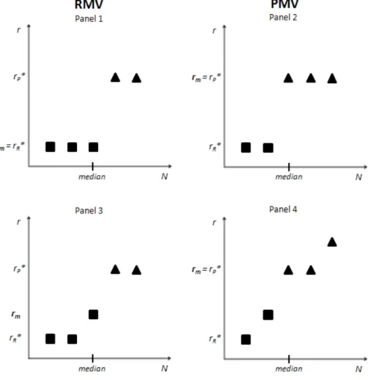
Figure 1 illustrates the basic intuition of the asymmetry effect in majority voting on redistribution for 5 voters in 2 income classes (see appendix B for the case of a continuum of voters in k classes). The vertical axis shows the redistribution level r and the horizontal axis ranks the voters by income class. The squares represent the ideal positions of rich voters, the triangles the ideal positions of poor voters. For example, panel 1 shows a case with 3 identical rich (self-interested) voters who have ideal points at rR* and 2 (self-interested) poor voters with ideal points at rP*. The panels on the left illustrate outcomes for rich majorities (RMV), the panels on the right for poor majorities (PMV). The upper panels show cases with self-interested voters, the lower panels cases where some voters are inequality averse.

Pocketbook voting by all voters (see upper panels) predicts dramatically different redistribution outcomes in RMV and PMV. If all voters cast their votes according to the

8

pocketbook, the median voter is rich in RMV and low redistribution at rm = rR* is the predicted outcome (see panel 1). In contrast, the median voter is poor in PMV, and an intermediate level of redistribution at rm = rP* is the predicted outcome (see panel 2).

The lower panels in figure 1 illustrate outcomes when some voters are inequality averse. Panel 3 illustrates the outcome in RMV where one rich voter is inequality averse and casts a vote ri > rR* while all others vote according to the pocketbook. In this case, inequality aversion does affect the redistribution outcome (rm > rR*). Panel 4 illustrates the case with a poor majority (PMV) where one poor voter and one rich voter is inequality-averse but the redistribution outcome is not affected by inequality aversion and the same outcome prevails in PMV as when no voter is inequality averse (rm = rP*).

Figure 1: Redistribution outcomes in majority voting for a rich majority (left panels) and poor majority (right panels), without (top) and with (bottom) inequality aversion (N = 5)

9

The asymmetry in redistribution outcomes prevails in the example above because with a narrow rich majority, the most inequality-averse rich voter drives the outcome (panel 3) but with a narrow poor majority, the least inequality-averse poor voter drives the outcome (panel 4). Thus, a little inequality aversion goes a long a way in RMV (this is the intuition discussed in Tyran and Sausgruber 2006), but is irrelevant in PMV.

Table 1: Probability of obtaining redistribution outcomes in line with standard theory (“pocketbook” prediction) with inequality-averse voters (ρ = 0.2)

1 2 3 4 5 6 7 8 # ri ch vot er s ( R ) 1 - 0.96 0.97 0.98 0.99 2 0.64 - 0.99 0.99 1.00 3 0.51 - 1.00 1.00 1.00 4 0.82 0.41 - 1.00 1.00 5 0.66 0.33 - 1.00 1.00 6 0.90 0.66 0.26 - 1.00 7 0.97 0.85 0.21 - 1.00 8 0.94 0.80 0.50 0.17 -

Table 1 illustrates how the asymmetry affect depends on the size of the electorate and the relative size of the two income classes in a simple simulation exercise. We assume that all N voters have single-peaked preferences and that their ideal points can be ordered as follows: self-interested rich (rR*) < inequality-averse rich < self-interested poor (rP*) < inequality-averse poor. That is, we assume that inequality aversion induces ideal points to shift in the direction of more redistribution, but only moderately so. To keep the argument simple, we assume that rich and poor voters are equally likely to be inequality averse (the argument can easily be extended to different probabilities across classes). In particular, we assume that voters are sampled from a population with a share of ρ percent inequality-averse voters. All voters are sincere and N is an odd number. If R > P (RMV), redistribution beyond the pocketbook obtains if at least xRMV = ½ (R – P + 1) inequality-averse rich voters are sampled into the electorate. If P > R (PMV), this is the case if at least xPMV = ½ (R + P + 1)

10

averse poor voters are sampled into the electorate. The main point to note here is that for any and . Thus, obtaining redistribution in excess of the standard prediction is more likely in RMV than in PMV.5

The probability of observing the pocketbook redistribution outcome, Prob(pocketbook), can be calculated using a binomial distribution (in table 1, we assume a share ρ = 0.2 of voters are inequality-averse). For example, in an electorate with R = 3 and P = 2, Prob(pocketbook) = (1 – ρ)³ = 0.51. In contrast, with R = 2 and P = 3, the probability is 1 – ρ3 = 0.99, i.e. the probability to observe the pocketbook outcome is about twice as large in the case of the poor majority. The numbers in table 1 below the main diagonal are for the case R > P. Importantly, these numbers are smaller than those above the diagonal for P > R which illustrates the asymmetry effect. That is, pocketbook redistribution outcomes are generally more likely with a poor majority than with a rich majority.

The asymmetry effect is particularly pronounced for “narrow” majorities. For example, holding the size of the electorate constant at N = 9, the probabilities to obtain the pocketbook outcome are essentially the same for R:P = 8:1 as for R:P = 1:8 (0.94 vs. 0.99) but the probabilities are much different for R:P = 5:4 and R:P = 4:5 (0.33 vs. 1.0). For a narrow rich majority, inequality aversion matters a lot while for the mirrored case with a poor majority it does not (the numbers above the diagonal are close to 1.0).

The asymmetry effect is particularly pronounced when inequality aversion looms large (ρ is large) and when the size of the electorate N increases. For example, if ρ = 0.3, Prob(pocketbook) is 0.34 for RMV (R = 3, P = 2) but still 0.97 for PMV. Thus, the asymmetry grows from about 2:1 (0.99 vs. 0.51, see table 1) with ρ = 0.2 to about 3:1 with ρ = 0.3. The asymmetry is also more pronounced in larger electorates as long as majorities are narrow. The asymmetry increases with N. For example, holding the ratio R:P constant at 3:2, the probability to obtain a pocketbook outcome is 0.51 with N = 5 but only 0.43 with N = 15 (not shown in the table).

5 _{Note that this statement pertains only to the probability of observing redistribution beyond the pocketbook.}

Additional assumptions on the intensity of inequality aversion would be needed to make precise statements about the extent of the deviation from pocketbook voting. For example, Fehr and Schmidt (1999) assume that spite is stronger than generosity which implies that the “poor” deviate by more from their ideal points than the rich, if they deviate at all.

11 Payoffs

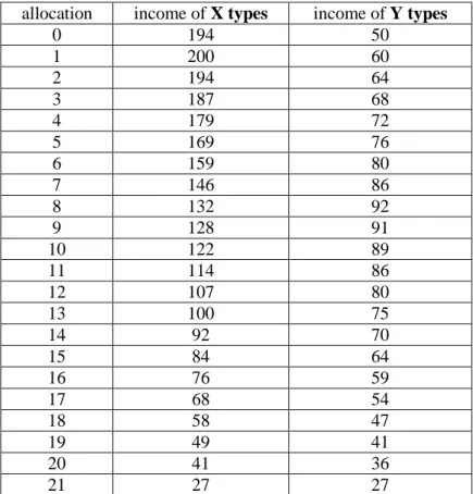
Table 2 shows the payoffs used in all 4 treatments by income class and redistribution level.6

Payoffs were chosen to reflect a trade-off between efficiency and equity. Figure 2 shows that redistribution decreases efficiency (the sum of the payoffs normalized to the sum of maximum payoffs) but increases equality (measured by the payoff of the poor relative to the rich). Rich voters maximize their income at low redistribution (rR* = 1), and poor voters at intermediate redistribution (rR* = 8).

The rich have higher maximum payoffs than the poor (200 vs. 92) and have higher payoffs at all redistribution levels except for the maximum redistribution level which equalizes incomes (payoff of 27 each). Note that payoffs are common information, i.e. all voters are mutually aware of the (private and social) tradeoffs involved, and there is no uncertainty over one’s (future) income position such that voting does not take place behind a “veil of ignorance” (see Cabrales, Nagel and Rodriguez Mora 2007 for an experimental study of social insurance).

7

Assuming pocketbook voting, a poor voter earns only about a third of a rich voter (= 60/200) in equilibrium in RMV. The equilibrium ratio of payoffs with PMV is more equal. At rP* = 8, the poor earn about 70 percent (= 92/132) of what the rich earn.

Table 2: Payoffs Redistribution level Payoff rich Payoff poor Redistribution Level Payoff rich Payoff poor 0 194 50 11 114 86 1 200 60 12 107 80 2 194 64 13 100 75 3 187 68 14 92 70 4 179 72 15 84 64 5 169 76 16 76 59 6 159 80 17 68 54 7 146 86 18 58 47 8 132 92 19 49 41 9 128 91 20 41 36 10 122 89 21 27 27 6

Instructions use neutral labeling. The “redistribution level” is called “allocation”, and the “rich” and the “poor” are called “x-type” and “y-type”, respectively.

7 _{Table 2 was part of the written instructions (see appendix A). The payoffs were calculated from a standard}

12

Inequality aversion may cause redistribution outcomes to deviate from rR* and rP*. For example, the poor may be spiteful and willing to sacrifice own payoff to reduce the payoff of the rich. However, doing so does not have much bite as can be seen in figure 2. For example, inequality is not reduced much by moving from r = 8 to 15 but comes at a hefty cost (about 1/3) in terms of efficiency. Thus, poor voters need to be strongly averse to inequality8 to find spiteful choices worthwhile. For the rich, generously giving up own payoff to increase payoffs of the poor (choices in {2,…,8}) is consistent with high values of β in the model of FS. However, redistribution beyond r = 10 implies β > 1, which is ruled out by assumption in the model of FS. In short, we do not expect redistribution outcomes above 8 given the inequality aversion typically assumed in the fairness model of FS.

Figure 2: Trade-off between efficiency and equality (vertical lines show redistribution outcomes according to pocketbook voting in RMV and PMV, respectively)

In total, 180 undergraduate students of various majors from the University of Innsbruck participated in the experiment as follows: 60 in RMV, 40 in PMV, 40 in RMRD and 40 in PMRD. Points earned during the experiment were exchanged at a rate of 200 points for 1 Euro. A show-up fee of 4 Euro was paid to all participants at the end of the experiment in

8

13

addition to earnings during the experiment. The experiment was programmed in zTree (Fischbacher 2007).

4. Results

Section 4.1 shows that redistribution in RMV is biased towards higher redistribution than predicted by pocketbook voting, but that redistribution is almost perfectly in line with pocketbook voting in PMV. Thus, we find pronounced asymmetry in how inequality aversion affects majority voting on redistribution. Section 4.2 shows that asymmetry is absent in the control treatments with a random dictator voting mechanism. Section 4.3 discusses that the asymmetry effect may induce insincere voting. We find that insincere voting increases with low pivotality according to the asymmetry hypothesis but is not pronounced enough to swamp the asymmetry effect.

4.1 The Pocketbook rules with PMV but not with RMV

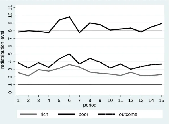
Figure 3 shows the main results for majority voting with a rich majority (RMV). We observe redistribution outcomes averaged across groups (rm, see dashed line) beyond the pocketbook prediction (rR* = 1, solid thin line) already in period 1 (p = 0.003, one-sample Wilcoxon signed-rank test, WSR), and rm remains at levels close to 4 throughout (average rm is 3.72 over all periods). The “excessive” redistribution is mainly due to the voting of the rich with an average vote of vR = 2.62 (p = 0.012, WSR). In contrast, voting of the poor is quite close to rP* = 8 (the average is vP = 8.40 over all periods; p = 0.209, WSR). The fact that rm is closer to vR than vP reflects the fact that the rich tend to be pivotal in RMV.9 The fact that rm > vR reflects that the inequality-averse rich tend to be pivotal, i.e. that they drive the redistribution outcome in RMV.10

9 _{Averaged over all periods, the distance to median in redistribution levels is 1.10 for the rich and 4.68 for the}

poor voters (p = 0.005, Wilcoxon matched pairs test, WMP).

In summary, the remarkable finding from RMV is that while the poor vote quite in line with standard theory, and the rich on average only deviate somewhat on the generous side, the average redistribution outcome is considerably more equal than predicted by pocketbook voting (index of inequality is 0.39 rather than 0.3 as predicted).

14

Figure 3: Average votes and redistribution outcomes in RMV (n = 60)

0 1 2 3 4 5 6 7 8 9 10 11 red is tr ib ut io n l e v el 1 2 3 4 5 6 7 8 9 10 11 12 13 14 15 period

rich poor outcome

Figure 4: Average votes and redistribution outcomes in PMV (n = 40)

0 1 2 3 4 5 6 7 8 9 10 11 red is tr ib ut io n l e v el 1 2 3 4 5 6 7 8 9 10 11 12 13 14 15 period

15

Voting is rather heterogeneous across the 12 electorates or groups in RMV. Overall, less than half (82/180) of the group-level outcomes are in line with pocketbook voting. While 5 groups have redistribution outcomes broadly in line with the standard prediction (i.e. deviate by 2 or fewer increments from rR* = 1.0), 7 groups are clearly not in line with standard predictions. Four of these groups implement intermediate levels of redistribution between 3 and 5 on average, while 3 groups have redistribution levels that are close to redistribution level 8. In one of these groups this is due to all three rich subjects consistently voting for r = 8, in the other two groups there are two and respectively one subject doing so. In these cases, the median voter gives up a payoff of 68 points (= 200-132, see table 1) to increase the income of the poor voters by 32 (= 92-60) points each. The choice reduced efficiency only by about 6 percent but considerably increased equality (the ratio of incomes of rich to poor falls from 3.3 to 1.4). While voting reduces inequality considerably, the resulting secondary income distribution is still rather unequal overall. The average payoff in the RMV treatment is (excluding the show-up fee) 13.2 Euro (rich) and 5.4 Euro (poor) (p = 0.000, two-sided Mann-Whitney test, MW).

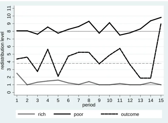
Figure 4 shows that redistribution outcomes are almost perfectly in line with pocketbook voting when the poor are in majority (PMV). Average redistribution is rm = 7.96 (see dashed line) which is very close to rP* = 8, and the prediction rP* = 8 is implemented exactly in 95 percent of the cases (= 114 out of 120 group-level observations). As a result, average total payoffs (excluding the show-up fee) are relatively equal in PMV (6.9 Euro for the poor and 9.9 Euro for the rich11). The redistribution outcome rm is close to but systematically below the graph representing the average vote vP of the poor (see solid black line) in PMV.12 The fact that rm is closer to vP than vR reflects that the poor tend to be the pivotal voters in PMV.13

The predictive success of standard theory assuming pocketbook voting for aggregate outcomes in PMV is striking because its predictions are rather imprecise if not plainly wrong for individual votes. The average vote of the rich is clearly biased away from their pocketbook optimum (rR* = 1) throughout all 15 periods (vR = 3.89, p = 0.012 WSR, see bold grey line in figure 4). In addition, a considerable share of the poor consistently vote above rP* The fact that rm < vP reflects that the inequality-averse poor are unlikely to be pivotal, i.e. tend not to drive the redistribution outcome.

11 _{The difference is nevertheless significant: p = 0.001, MW.}

12 _{7.96 vs. 8.88, p = 0.019, WMP.}

13 _{The average (absolute) distances are r}

16

= 8 and the average vote over all periods is vP = 8.88 (p = 0.019 WSR, see bold black line in figure 4). While only 53 percent of all voters (18 poor and 3 rich) vote their pocketbook interest in at least 2/3 of the periods, the redistribution outcome is almost always (in 95 percent of group-level outcomes) consistent with standard theory. Thus, in line with the asymmetry hypothesis, we find that – despite many voters supporting redistribution beyond the pocketbook – inequality aversion does not matter for aggregate outcomes when the poor are in majority.

4.2 Results from random dictator treatments

We now show that there in fact is no asymmetry in the deviation from pocketbook outcomes across class structures when there should be none according to the asymmetry hypothesis. To test, we run treatments with an exogenous and constant probability to be decisive. Importantly, the probability is the same (1/N = 0.2) for all voters in both treatments, i.e. does not depend on which class is in majority. We implement two treatments with random dictator decision making. Treatment RMRD has a rich majority, and treatment PMRD has a poor majority. Note that these treatments are identical to RMV and PMV in all respects except for the voting rule. Our main finding is that the deviation from pocketbook outcomes is not different across treatments, i.e. is independent of which class is in majority.

Figures 5 and 6 show the average redistribution choice by income class for random dictator voting in RMRD and PMRD. Both the poor and the rich make random dictator choices slightly above predictions in PMRD (dP = 8.56 vs. rP* = 8, p = 0.030; dR = 1.50 vs. rR* = 1, p = 0.030, WSR). In RMRD average choices are not significantly different from predictions (poor: 8.40 vs. 8, p = 0.356; rich: 1.28 vs. 1, p = 0.110, WSR).

17

Figure 5: Average votes and redistribution outcomes in RMRD (n = 40)

0 1 2 3 4 5 6 7 8 9 10 11 red is tr ib ut io n l e v el 1 2 3 4 5 6 7 8 9 10 11 12 13 14 15 period

rich poor outcome

Figure 6: Average votes and redistribution outcomes in PMRD (n = 40)

0 1 2 3 4 5 6 7 8 9 10 11 red is tr ib ut io n l e v el 1 2 3 4 5 6 7 8 9 10 11 12 13 14 15 period

18

The heavily dashed lines in figures 5 and 6 show the implemented redistribution in the two treatments. Implemented redistribution is noisy because one choice is picked at random to determine the outcome in these treatments, and the choice may come from a rich or a poor voter. Importantly, we find that the deviation of predicted and implemented redistribution is not different across treatments. The pocketbook prediction rd* is 5.20 in PMRD and 3.80 in RMRD (see dashed horizontal lines). These predictions differ from those in RMV and PMV because of a simple composition effect [note that rd* = (R . rR* + P . rP*) / N)]. Overall (weighted) dictator choices are rd = (R . dR + P . dP) / N. The absolute deviation rd – rd* is 1.14 in PMRD (6.34 vs. 5.20), and 0.57 in RMRD (4.37 vs. 3.80), and these deviations are not significantly different (p = 0.371, MW). In contrast, the deviations from predicted outcomes are significant with majority voting. i.e. across RMV and PMV. The deviation rm – rR* is 2.72 in RMV (3.72 vs. 1) and rP*– rm = -0.04 in PMV (7.96 vs. 8), which is significantly different (p = 0.001, MW). In summary, the deviations between predicted and observed redistribution outcomes are small (about 0.6) and do not differ across treatments in the random dictator procedure, but deviations are large (about 2.8) and significant in the majority voting treatments.

Our finding that the deviation of implemented redistribution from the pocketbook prediction does not differ across treatments when pivotality is independent of class structure also holds for individual choices. This is true for both rich and poor voters, and for both the level and the variance of choices. A comparison of PMRD vs. RMRD reveals that neither rich voters (1.50 vs. 1.28, p = 0.419, MW) nor poor voters (8.56 vs. 8.40, p = 0.522, MW) choose differently across these treatments on average. The average within-group standard deviation for rich voters is 0.74 in PMRD and 0.55 in RMRD (p = 0.957, MW). For the poor voters the respective numbers are 0.77 vs. 1.31 (p = 0.394, MW).

4.3 Discussion of results: insincere voting

The asymmetry hypothesis claims that sincere voting for redistribution beyond the pocketbook by a given share of inequality-averse voters is more or less likely to translate into redistribution outcomes beyond pocketbook interests depending on how likely inequality-averse voters are to be pivotal; pivotality, in turn, depends on the relative strength of income classes. The discussion above has shown that we find support for the asymmetry hypothesis in majority voting in the sense that aggregate redistribution outcomes are much less in line with

19

standard predictions in RMV than in PMV. This holds both with respect to overall average redistribution levels and with respect to group-level outcomes. For example, 46 vs. 95 percent of group-level outcomes are in line with standard predictions in RMV and PMV, respectively.

These results are surprising because voters may anticipate and respond to the differential pivot probabilities by voting insincerely. For example, rich voters may anticipate that they are more likely to be pivotal when they are in majority (in RMV) than when they are not (in PMV). Not to vote for the income-maximizing choice is thus less costly in PMV than in RMV. Voters may react to these differences in expected cost by voting carelessly (thus increasing the noise) or by expressing support for what may be seen as a morally worthy cause (thus increasing the bias towards redistribution beyond the pocketbook prediction). Note that incentives for insincere voting are completely absent in the treatments with random dictator choice.

A comparison of voting patterns across RMV and PMV reveals that insincere voting is indeed more common for rich voters when they are less likely to be pivotal but the evidence is weak for poor voters. For example, among the rich, we find that 57 percent (= 309/540) of individual votes are in line with the pocketbook interests (rm* = 1) in RMV but only 32 percent (= 76/240) are in PMV. The difference is significant (p = 0.000, χ2 test). Yet, insincere voting among the rich mainly increases noise rather than the average vote.14 Similar results hold for poor voters.15

Insincere voting may also explain some of the apparent differences in individual choices across voting rules. However, the comparison is less sharp in this case. The reason is that while we control the pivot probability in the random dictator treatments (it is 0.2), the absolute level of that probability is not known in the voting treatments. We do know from the asymmetry hypothesis that this probability is higher for rich voters in RMV than PMV. But we do not know whether 0.2 is between or, say, below both of these probabilities.16

14

In RMV, the average within-group standard deviation of votes among the rich is less than half that of PMV

(1.06 vs. 2.29, p = 0.021, MW, based on a comparison of 12 and 8 independent group observations in RMV

and PMV, respectively). But the average vote of the rich is not significantly different between RMV and in

PMV (2.62 vs. 3.89, p = 0.123, MW).

15

As for the rich, poor voters are more likely to vote insincerely when they are in minority: 51% (= 183/360)

and 78% (= 281/360) of poor voters vote in line with pocketbook in RMV and PMV, respectively. p = 0.000,

χ2 _{test. While the average within-group standard deviation of votes is higher in RMV than PMV (2.12 vs.}

0.22, p = 0.002, MW), average votes do not differ across the treatments (8.40 vs. 8.88, p = 0.396, MW).

16

For completeness, we note that for the rich both the average (3.89 vs. 1.50, p = 0.007, MW) and the standard

deviation (2.29 vs. 0.74, p = 0.027 MW) are different across PMV than PMRD. Neither is the case for the

poor voters (8.88 vs. 8.56, p = 0.958, MW; 0.77 vs. 0.22, p = 0.388, MW). There are no differences in levels

20

5. Concluding remarks

A burgeoning literature has convincingly shown that concerns for a fair distribution are common but little attention has been devoted to how it may affect voting on redistribution. Whether fairness concerns matter for redistribution outcomes in majority voting depends on whether inequality-averse voters are pivotal. Pivotality, in turn, depends on the income class structure of the electorate and we show that its effect is asymmetric. Our results support the idea that a given amount fairness concerns matter when few fair-minded voters are sufficient to tip the balance in majority voting, but does not matter much when many are needed.

While the asymmetry effect extends to redistribution in electorates with more than two income classes in theory, we would like to caution the reader to extrapolate the willingness to redistribute beyond the pocketbook observed in our study because the concern for fairness manifest in our experiment may not be typical for other samples. For example, Alesina and Giuliano (2009) note that different cultures emphasize the relative merits of equality versus individualism in different ways, and different historical experiences shape social norms about what is acceptable in terms of inequality (for a study of cultural effects on cooperation see Herrmann, Gächter and Thöni 2008). Another interesting alley for further experimental investigation is how fair-minded voting is shaped by the conditions that can be controlled in an experiment. For example, voting for inequality-reducing redistribution may be less common when incomes are earned and voters therefore feel entitled to their incomes (Fong 2001 for survey evidence; for moral property rights in Ultimatum games, see e.g. Gächter and Riedl 2005. See Cappelen et al. 2010 for dictator games with production, Esarey et al. 2011 for voting on redistribution). On the other hand, voting for inequality-reducing redistribution may be more common when the trade-off between efficiency and equality is less pronounced than in our design because preferences for efficient outcomes seem to be common (e.g. Charness and Rabin 2002). Indeed, Durante and Putterman (2009) provide direct evidence showing that the support for redistribution decreases with its private and social cost.

In a broader perspective, our paper adds to an emerging literature discussing the conditions when fairness concerns in a heterogeneous population matter for aggregate outcomes (e.g. Dufwenberg et al. 2008, Sobel 2009, Schmidt 2010). One way to read our results is as a kind of “robustness test” of the standard median voter theory. Our results suggest that fairness preferences may matter much or be essentially irrelevant for majority voting on redistribution. Which effect prevails depends, according to our analysis, on the

21

structure of income classes which can be reasonably well measured in the field. Thus, we believe our experimental finding provides interesting directions for field research. Our results suggest that relating (easily observable) redistribution outcomes to particular (easily observable) aspects of the structure of income classes may provide a promising new perspective to investigating the role of (only indirectly observable) fairness preferences in democratic redistribution.

References

Ackert, L.F., Martinez-Vazquez, J. and Rider, M. (2004): Tax Policy Design in the Presence of Social Preferences: Some Experimental Evidence. Working Paper 2004-33, Federal Reserve Bank of Atlanta.

Alesina, A.F. and Giuliano, P. (2009): Preferences for Redistribution. NBER working paper 14825.

Battaglini, M., Morton, R.B. and Palfrey, T.R. (2010): The Swing Voter’s Curse in the Laboratory. Review of Economic Studies 77(1): 61-89.

Beckman, S.R., Formby J.P. and Smith, W.J. and Zheng (2002): Envy, Malice and Pareto Efficiency: An Experimental Examination. Social Choice and Welfare 19: 349-67. Bellemare, C., Kröger, S. and van Soest, A. (2008): Measuring Inequity Aversion in a

Heterogeneous Population using Experimental Decisions and Subjective Probabilities. Econometrica 76(4): 815-39.

Bolton, G. and Ockenfels, A. (2000): ERC: A Theory of Equity, Reciprocity, and Competition. American Economic Review 90(1): 166-93.

Bolton, G. and Ockenfels, A. (2003): The Behavioral Tradeoff between Efficiency and Equity when a Majority Rules: Max Planck Institute of Economics, Strategic Interaction Group Discussion Paper.

Cabrales, A., Minaci, R., Piovesan, M. and Ponti, G. (2010): Social Preferences and Strategic Uncertainty: An Experiment on Markets and Contracts. American Economic Review 100(5): 2261-78.

22

Cabrales, A., Nagel, R. and Rodiguez Mora, J.V. (2007): It’s Hobbes, not Rousseau: An Experiment on Social Insurance. Working paper Labsi Experimental Economics Laboratory University of Siena, University of Siena.

Camerer, C.F. (2003): Behavioral Game Theory: Experiments in Strategic Interaction. Princeton University Press.

Cappelen, A.W., Sørensen, E.Ø. and Tungodden, B. (2010): Responsibility for What? Fairness and Individual Responsibility. European Economic Review 54(3): 429-41. Charness, G. and Kuhn, P.J. (2010): Lab Labor: What Can Labor Economists Learn from the

Lab? NBER Working Paper No. 15913.

Charness, G. and Rabin, M. (2002): Understanding Social Preferences with Simple Tests. Quarterly Journal of Economics 117(3): 817-69.

Dhami, S. and Al-Nowaihi, A. (2010): Redistributive Policies with Heterogeneous Social Preferences of Voters. European Economic Review 54(6): 743-59.

Downs, A. (1957): An Economic Theory of Democracy. New York: Harper and Row. Dufwenberg, M., Heidhues, P., Kirchsteiger, G., Riedel, F. and Sobel, J. (2011):

Other-Regarding Preferences in General Equilibrium. Review of Economic Studies 78(2): 613-39. Durante, R. and Putterman. L. (2009): Preferences for Redistribution and Perception of

Fairness: An Experimental Study. Mimeo (July 30, 2009).

Eichenberger, R. and Oberholzer-Gee, F. (1998): Rational Moralists: The Role of Fairness in Democratic Economic Politics. Public Choice 94(2): 191-210.

Engelmann, D. and Strobel, M. (2004): Inequality Aversion, Efficiency, and Maximin

Preferences in Simple Distribution Experiments. American Economic Review 94(4): 857-69. Esarey, J., Salmon, T.C. and Barrilleaux, C. (2011): What Motivates Political Preferences?

Self-Interest, and Fairness in a Laboratory Democracy. Economic Inquiry, forthcoming. Feddersen, T.J., Gailmard, S. and Sandroni, A. (2009): Moral Bias in Large Elections: Theory

and Experimental Evidence. American Political Science Review 103(2): 175-92.

Fehr, E., Goette, L. and Zehnder, C. (2009): A Behavioral Account of the Labor Market: The Role of Fairness Concerns. Annual Review of Economics 1: 355-84.

Fehr, E. and Schmidt, K. (1999): A Theory of Fairness, Competition and Cooperation. Quarterly Journal of Economics 114(3): 817-68.

Fehr, E. and Tyran, J.-R. (2005): Individual Irrationality and Aggregate Outcomes. Journal of Economic Perspectives 19(4): 43-66.

23

Fischbacher, U. (2007): Zurich Toolbox for Readymade Economic Experiments. Experimental Economics 10(2): 171-8.

Fong, C. (2001): Social Preferences, Self-interest, and the Demand for Redistribution. Journal of Public Economics 82: 225-46.

Gächter, S. and Riedl, A. (2005):Moral Property Rights in Bargaining with Infeasible Claims. Managment Science 51(2): 249-63.

Galasso, V. (2003): Redistribution and Fairness: A Note. European Journal of Political Economy 19(4): 885-92.

Grosser, J. and Reuben, E. (2009): Redistributive Politics and Market Efficiency: An Experimental Study. IZA Working paper 4549.

Hermann, B., Gächter, S. and Thöni, C. (2008): Antisocial Punishment Across Societies. Science 319: 1362-7.

Kamenica, E. and Egan, L. (2011): Voters, Dictators, and Peons: Expressive Voting and Pivotality. Mimeo (June 2011).

Klor, E.F. and Shayo, M. (2010): Social Identity and Preferences over Redistribution. Journal of Public Economics 94(4): 269-78.

Lewis-Beck, M.S. and Stegmaier, M. (2007): Economic Models of the Vote. InR. Dalton and H.-D. Klingemann (eds.): The Oxford Handbook of Political Behavior. Oxford: Oxford

University Press: 518–37.

Meltzer, A.H. and Richard, S.F. (1981): A Rational Theory of the Size of Government. Journal of Political Economy 89(5): 914-27.

Schmidt, K. (2010): Social Preferences and Competition. Munich Discussion paper 2010-6. Shayo, M. and Harel, A. (2011): Non-consequentialist Voting. Mimeo (March 2010) Sobel, J. (2009): Generous Actors, Selfish Actions: Markets with Other-Regarding

Preferences. International Review of Economics 56: 3-16.

Tyran, J.-R. (2004): Voting when Money and Morals Conflict. An Experimental Test of Expressive Voting. Journal of Public Economics 88(7): 1645-64.

Tyran, J.-R. and Sausgruber, R. (2006): A Little Fairness may Induce a Lot of Redistribution in Democracy. European Economic Review 50(2): 469-85.

24

Appendix A: Sample Instructions

Welcome to the experiment. If you read these instructions carefully and follow the rules you can earn money in this experiment. The money will be paid out in cash right after the experiment. During the experiment, we denote earnings in points which are converted to Euro as follows: 200 points = 1 Euro.

You are not allowed to communicate with other participants during the entire experiment. If you have a question, please raise your hand and we will answer your question individually. It is important that you follow this rule because otherwise the results are worthless to us.

In this experiment, participants are randomly sorted into groups of 5. This means that you are in a group with 4 other participants. The same 5 participants stay in a group throughout the entire experiment.

In your group, there are 2 members of type Y and 3 members of type X. The computer randomly determines who is of which type.

What are the consequences of being type X or type Y? Players of type X have better

opportunities to earn money in the experiment.

In this experiment, your task is to decide about the distribution of incomes within your group.

Specific instructions for the experiment

You are of type Y. In this experiment, every participant earns an individual income. You

vote about whether and to what extent you would like to redistribute these incomes by choosing an “allocation”.

The experiment has 15 periods in total. In each period, you have to vote about the redistribution of the incomes in your group. The outcome of the vote in each period determines your and the other 4 group members’ payoff.

Redistribution decision

Table 1 shows the incomes for each allocation. There are 22 possible allocations in total. You and the other participants in your group decide about the allocation for your group and thus about the distribution of incomes in your group.

[For treatments RMV and PMV] The redistribution decision is made according to the

following rules: You and the other group members each choose an allocation by typing an allocation number into the decision screen that will pop up. The allocation numbers chosen by all group members are sorted from low to high. The number in the middle, i.e. the third number, in this list is the median allocation. The median allocation determines the incomes of all group members in this period (see table 1).

Example: Suppose you have chosen allocation 12. The other four group members have

chosen allocations: 11, 2, 17, 5. Sorted from low to high we have: 1: 2

2: 5

3: 11 (= median allocation) 4: 12

5: 17

The median allocation and, thus, the group’s redistribution decision, in this example is 11 which means that X types earn 114 points and Y types earn 86 points.

25

Suppose you had chosen 8 instead of 12 in the situation above while the others choose as before (11, 2, 17, 5). In this case, your allocation choice is the third in the sequence. Therefore, the median allocation would be 12 and the group’s redistribution decision is therefore 12 which means that X types earn 107 points and Y types 8 points.

[For treatments RMRD and PMRD]: The redistribution decision is made according to

the following rules: You and the other group members each choose an allocation by typing

an allocation number into the decision screen that will pop up. The computer then randomly

draws one of these allocations with equal probability (20%). The random draw from the

choices determines the incomes of the group members in this period (see table 1).

Example: Suppose you choose allocation 12. The other members of your group choose the

allocations: 11, 2, 17, 5. The computer draws one of these 5 allocation randomly and all allocations are equally likely to be implemented. For example, if allocation 11 is drawn, all group members obtain the income shown for allocation 11 in table 1 (114 points for X types and 86 points for Y types).

[all treatments]

Table 1: Incomes for different allocations

allocation income of X types income of Y types

0 194 50 1 200 60 2 194 64 3 187 68 4 179 72 5 169 76 6 159 80 7 146 86 8 132 92 9 128 91 10 122 89 11 114 86 12 107 80 13 100 75 14 92 70 15 84 64 16 76 59 17 68 54 18 58 47 19 49 41 20 41 36 21 27 27

How you make your decision: In each period, you choose an allocation by typing a fumber

from 0 to 21 into the decision screen. When all group members have made their decisions, the group choice is determined and displayed. At the end of the period you will see the following information on the outcome screen: [You are type …, The group’s allocation decision is …, Your income is …, Group members of type X earned …, group members of type Y earned …]

26

Appendix B: Asymmetry with k > 2 income classes

Our reasoning adapts the standard model of redistribution by Meltzer and Richard (MR 1981) in which voters have single-peaked preferences for redistribution in a single dimension. MR has voters with different labor productivities which map into different levels of labor income. Voting is on a uniform tax on labor income and per capita redistribution with the effect that redistribution reduces inequality. Because workers are assumed to choose labor supply optimally, redistribution is associated with disincentive effects. As a consequence, there is a trade-off between equality and efficiency. In MR, voting is compulsory and sincere. Voters are self-interested and vote for the level of redistribution that maximizes their post-redistribution income, correctly anticipating the disincentive effects from equilibrium redistribution. As a result, high-income voters vote for low redistribution while low-income voters vote for intermediate (rather than maximum) levels of redistribution. In equilibrium, the preference of the median voter (which is driven by his labor productivity) determines the redistribution outcome.

In contrast to MR, we assume that voters are grouped in income classes (i.e. non-singleton subsets of voters with identical incomes) and that voters are heterogeneous with respect to inequality aversion. Both assumptions are essential for our argument and discussed in detail below. We use a reduced-form version of the MR model in that we solve for optimal labor supply for given redistribution levels. The payoffs shown in Table 1 can thus be derived from a reduced-form MR model17

(i) Income classes: Assume a continuum of voters with a mass normalized to 1. Each voter is a member of income class k = 1,..., q. Each class contains a share of the electorate mk (

assuming an electorate of 5 voters, homogenous classes of high-productive (“rich”) and low-productive (“poor”) workers / voters, discrete levels of a flat tax with per capita redistribution, and optimal labor supply decisions. The discussion below generalizes this case to a continuum of voters and finitely many income classes.

). Voters choose among a discrete set R = {1,…, l} of redistribution policies. For each income class k there is a unique redistribution policy that maximizes post-redistribution income and the median policy rmed is implemented for all voters. Voters from a poorer class (high k) demand more redistribution: . We denote by the income of a voter in class k for redistribution policy r and make the following assumptions:

17 _{MR implies monotonically falling post-redistribution incomes for rich voters. We chose to implement an}

interior maximum at r = 1 for experimental reasons, in particular to allow for the possibility that small

27

A1: .

A2: .

A3: .

A1 states that a voter’s income is maximized at a unique r* which increases with k. A2 states that redistribution is inequality-reducing, i.e. that the difference of incomes between classes decreases with r. A3 says that redistribution is non-revolutionary since the ordering of income classes is preserved at all levels of redistribution.

(ii) Inequality aversion: Assume that voters are heterogeneous with respect to inequality aversion. A self-interested voter demands By assumption A3, an inequality-averse voter demands more redistribution than an otherwise identical, purely self-interested voter:

. The further away the ideal policy is from the self-interested optimum, the stronger is the voter’s inequality aversion.

We assume that each voter is inequality averse with some probability and that more extreme levels of inequality aversion are less common than moderate levels. Let denote the probability that policy r is drawn for a voter of class k. The following assumptions characterize the voters’ probability distributions over R:

A4:

A5: .

A6: .

A4 rules out that voters prefer inequality, i.e. they are not willing to sacrifice income to make the distribution more unequal. A5 says that voters are most likely to be self-interested, and, if they are inequality-averse, extreme inequality aversion is less likely than moderate. A6 says that voters do not abstain.

We capture the assumption in MR that higher levels of redistribution are increasingly costly with increasing pre-redistribution income (disincentive effects increase with falling k) by assuming that rich voters are less likely to prefer a given high-redistribution policy r than the poor (high k):

A7:

Due to the law of large numbers, a discrete probability distribution over the countable set R translates into shares of voters who cast a vote for policy . Call

28

the mass of voters in class k who vote for policy r, and call the total mass of voters in the society for whom r is drawn. The implemented policy, rmed, is found by summation of Mr over classes starting with the richest class ( ) until the median position (at 1/2 of the mass of voters) is reached:18

(iii) Political equilibrium: Before characterizing the political equilibrium with inequality-averse voters formally, it is useful to illustrate the intuition. Figure B1 shows a distribution of votes over the policy space R with 10 levels of redistribution ( ) and 5 income classes ( ).19

Panel 1 illustrates the reference case in which all voters are strictly self-interested and cast their votes sincerely according to the pocketbook. In this case,

The vertical axis shows the level of redistribution and the horizontal axis shows the cumulated mass of voters sorted by income. The richest voters are in class 1 (far left) followed by the second richest in class 2, etc. In each panel, the length of the horizontal lines measures the mass of voters who prefer a particular level of redistribution. Thus, a line further up indicates that the voters in this class prefer more redistribution, a longer line indicates that there are many voters in this class.

is implemented (the median position is indicated by the dotted vertical line). Panel 2 illustrates the case where about half of the voters in each class is inequality averse to various degrees. Segments of the lines are thus shifted upwards in panel 2. The political equilibrium is found by cumulating the distribution of the votes. Panel 3 shows that median position intersects this cumulated distribution at level . Thus, the presence of inequality aversion increases the equilibrium redistribution in this example from level 3 to 5. Note that only inequality aversion of voters from the median or richer classes matters for the policy outcome. 20

18 _{We can think of the median vote beating all other r in pair wise majority voting. Formally this requires that}

preferences over R are single-peaked for the realized type of each voter.

19 _{The number of classes, their sizes, the number of redistribution policies etc. in figure 1 are all arbitrarily}

chosen.

20 _{The distribution of votes in the class(es) above k}

med does not matter for whether the implemented policy is

beyond the pocketbook interest of kmed. It may matter, however, for how much the implemented distribution

29

30

Figure B1 illustrates a case where “sufficiently many” voters from the median and richer classes are fairness-minded to move the median towards higher levels of redistribution. Formally, “sufficiently many” means that at least x voters from these classes vote for redistribution in excess of . Graphically, x is the distance between the median voter position and that of the marginal voter of the median class. Call kmed the class containing the median voter and the materially optimal policy for the voters in the median class.

Formally, . If x is small, a little fairness may suffice to change the prediction of the standard model. The larger x, the higher the required share of inequality averse voters to change voting outcomes. Generally, the necessary and sufficient condition for a fair outcome is

FigureB2: Share of fair voters (z) necessary for fair outcomes as function of x

The required share of fair voters within the median and richer classes to induce an aggregate outcome beyond what is predicted by income maximization can also be written as

, see Figure B2. If x is zero, an arbitrarily small share of sufficiently inequality averse voters in classes 1 to kmed is sufficient to induce redistribution beyond the standard pocketbook outcome.21 At x = 0.5, which implies that the median class is also the poorest class, a fair voter is pivotal only if at least 50% of the electorate is sufficiently fair-minded.22

21 _{“Sufficiently inequality averse” means that a voter prefers redistribution beyond what is materially optimal for}

voters in the median class.