Credit default swaps and systemic risk
∗Rama Cont†, Andreea Minca‡ August 2014.
Abstract
We present a network model for investigating the impact on systemic risk of central clearing of over the counter (OTC) credit default swaps (CDS). We model contingent cash flows resulting from CDS and other OTC derivatives by a multi-layered network with a core-periphery structure, which is flexible enough to reproduce the gross and net exposures as well as the heterogeneity of market shares of participating institutions. We analyze illiquidity cascades resulting from liquidity shocks and show that the contagion of illiquidity takes place along a sub-network consituted by links identified as ’critical receivables’.
We calibrate our model to data representing net and gross OTC exposures of large dealer banks and use this model to investigate the impact of central clearing on network stability. We find that, when interest rate swaps are cleared, central clearing of credit default swaps through a well-capitalized CCP can reduce the probability and the magnitude of a systemic illiquidity spiral by reducing the length of the chains of critical receivables within the financial network. These benefits are reduced, however, if some large intermediaries are not included as clearing members.
Keywords: Systemic risk, financial networks, multi-layered network, credit default
swaps, financial crisis, intermediation chains, financial stability.
∗
We thank seminar participants at the Mathematical Modeling of Systemic Risk Workshop (Paris, June 2011), the IMF Workshop on Systemic Risk Monitoring (2010), the Capital Markets Function Seminar (NY Fed, December 2011), the Research in Options Conference (Buzios 2011), Information and Econometrics of Networks Workshop (Washington DC, 2012) and the Symposium on Critical Challenges at the Interface of Mathematics and Engineering (2012) for helpful discussions. We acknowledge the hospitality of the Isaac Newton Institute for Mathematical Sciences for support and hospitality during the programme onSystemic Risk: Mathematical
Modeling and Interdisciplinary Approaches.
†
Imperial College London & Laboratoire de Probabilit´es et Modeles Al´eatoires, CNRS-Universit´e Pierre & Marie Curie. email: [email protected]
‡
School of Operations Research and Information Engineering, Cornell University, Ithaca, NY 14850, USA, email: [email protected]
Contents
1 Introduction 2
2 Over-the-counter markets 5
3 A network model for contingent OTC exposures 9
3.1 Payables and receivables . . . 9
3.2 A network model for OTC exposures . . . 11
3.2.1 A matching model for non-CDS exposures . . . 12
3.2.2 A multi-layered network model for CDS exposures . . . 13
3.3 Calibration results for a sample OTC network . . . 15
4 Does central clearing of CDS reduce systemic risk? 17 4.1 Resilience to illiquidity cascades in stress scenarios . . . 17
4.2 The stress scenario . . . 18
4.3 Simulation results . . . 20
5 Conclusions 22
1
Introduction
The role played by the multi-trillion dollar market for credit default swaps (CDS) and other over-the-counter (OTC) credit derivatives in the recent financial crisis, especially in the demise of AIG, has prompted many discussions on the impact of CDS on financial stability and systemic risk ([Cont, 2010, Stulz, 2010]) and led to various regulatory initiatives, the most well-known being the requirement of mandatory clearing for standardized CDS contracts, introduced in the Dodd-Frank Act in the US and in the EMIR framework in Europe.
Given the cost and effort involved in implementing these central clearing mandates, a valid question is whether they can be expected to achieve their objective, which is to mitigate systemic risk in the financial system. While recent studies by regulators tend to answer this question in the affirmative [Macroeconomic Assessment Group on Derivatives (MAGD), 2013], it is of interest to dispose of independent studies which tackle the question in a more general setting using a transparent methodology.
The impact of central clearing of OTC derivatives has been studied by [Duffie and Zhu, 2011, Cont and Kokholm, 2014, Heller and Vause, 2012, Sidanius and Zikes, 2012] and [Duffie et al., 2014], mainly through the angle of the (aggregate) level of counterparty exposures and the resulting demand in collateral.
The central insight in these studies is that the impact of central clearing on the level of ex-posures crucially depends on the tradeoff between bilateral netting across derivative classes and multi-netting via the clearing house. The tradeoff is assessed based on the average exposure un-der the different netting and clearing arrangements, and is shown to depend on the characteristic of the network, in particular the correlation of exposures across asset classes and the riskyness of these exposures [Duffie and Zhu, 2011, Cont and Kokholm, 2014]. [Farboodi, 2014] proposes a
stylized model for the endogenous formation of intermediation links among debt financed banks whose equilibria correspond to core-periphery network structures: all equilibria lead to exces-sive counterparty exposures and central clearing can be welfare-improving. [Amini et al., 2013] examine central clearing from the point of view of optimal design of the CCP waterfall.
However, these studies focus on the average (or aggregate) level of counterparty exposures and it is not clear what this metric has to say about systemic risk resulting from the net-work’s response to a stress scenario. Indeed, as underlined in recent studies on contagion in financial networks, what determines the magnitude of contagion stemming from a default in a counterparty network is not only the aggregate level of exposures but above all the way these ex-posures are distributed across links in the network, and their relation to the capital or liquidity buffer held by financial institutions ([Watts, 2002, Gai and Kapadia, 2010, Amini et al., 2011, Cont et al., 2013]).
A natural framework for tackling these questions is a network model; such models have been extensively used for analyzing contagion and systemic risk in financial system. Most existing models used for analyzing financial networks aggregate all bilateral exposures for a given pair of counterparties into a single number, the net exposure attached to the corresponding link. However, unlike other OTC derivatives, exposures due to CDS may exhibit large variations (’jumps’) contingent on a credit event -whether a default or a downgrade- which may generate large margin calls: these ’contingent liquidity shocks’ resulting from CDS transactions are not exogenous to the network but triggered by the default of nodeswithinthe network.
The structure of the OTC network models- in particular in terms of concentration and connectivity- needs to reflect the actual structure of OTC exposures between financial insti-tutions. Although some data sets on bilateral OTC notionals have started to be explored by regulators (see for example the interesting study by [Peltonen et al., 2014]), these data sets do not contain any information on collateral levels and thus do not give any precise information
on exposures which are, of course, the key quantity of interest in any network model. Thus,
there is a need for models which can ’fill the gaps’ in the data and generate realisticexposure
networksfor stress testing and simulation purposes.
The network structure of the OTC market reveals a core of large dealer banks that act as in-termediaries among customers (or end-users) [ECB, 2009, Peltonen et al., 2014]. Such dealers may choose in many cases to hedge their exposures to end-users and enter offsetting contracts with other dealers, leading to intermediation chains [Zawadowski, 2013, Farboodi, 2014]. The
OTC network can be seen then as the superposition of these intermediation chains [Glode and Opp, 2013]. The presence of such intermediation chains means that if one large end-user or intermediary
defaults, this default may propagate along the chain of intermediaries through an illiquidity cascade: when some firms in the intermediation chain do not hold enough liquidity to cover their payables, counterparties for which those receivables are critical in order to meet their own payment obligations become illiquid themselves.
The liquidity shocks generated by credit events are further amplified by the large concen-tration of the CDS market on intermediaries. Indeed, in the CDS market, a few protection sellers concentrate the large majority of transactions [ECB, 2009]. These protection sellers will immediately face a liquidity shortage if the spreads of reference entities across a given sector move up or down at the same time.
each layer contains all CDS exposures references on the default of a given reference entity. This representation, rather than aggregating the mark-to-market values of all CDS into a single bilateral exposure, allows to model the change in CDS exposures triggered by a credit event, which is a necessary step in simulating the response of the network to a credit event in a stress scenario.
We show that our network model can accomodate these empirically observed features of the CDS market in a realistic way : the underlying network of financial institutions has a core-periphery structure1, in which we distinguish dealer bank from other market participants, and the model is flexible enough to reproduce the heterogeneity in market share and the asymmetries in exposures implied by observed values of gross vs net CDS notionals. We illustrate the flexibility of the model by calibrating it to the data on the gross and net CDS protection sold on the top 1000 names recently published by The Depository Trust and Clearing Corporation (DTCC) [DTCC, 2010], as well as on the market share of the dealers2.
Next, we describe how liquidity shocks -in particular those arising from credit events- propa-gate through this networks and how, in some situations, may lead to contagion via an illiquidity cascade. We show that this contagion is concentrated on the subnetwork of ’weak links’ which correspond to ’critical receivables’ and exhibit an indicator of the network’s resilience to this illiquidity contagion, introduced in [Amini et al., 2011], which allows a simulation-free analysis of the degree of resilience of the network to liquidity shocks. In particular, we show that this indicator can be used to detect thetipping-point, orphase transition, which is the critical level of liquidity shock which leads to a regime where illiquidity contagion becomes large scale.
Finally, we apply these concepts to analyze the impact of central clearing of credit de-fault swaps on financial stability. Using simulations and analytical insights from large-network asymptotics, we explore the impact of introducing a CDS clearinghouse on the extent of distress propagation in the network. Our analysis shows that, in a network where other major OTC derivatives (primarily IR swaps) are cleared, the addition of a CDS clearing facility enhances network stability and a significantly larger shock is necessary to trigger a phase transition. On the other hand, in absence of clearing of the other classes of OTC derivatives, central clearing of CDS may have negative impact on financial stability. The presence of a well-capitalized CDS clearing facility is shown to increase the resilience of the network provided that all significant intermediairies are clearing members: in this case, the CCP significantly shortens the inter-mediation chains. However, the impact of the CCP on network stability is weakened if some major intermediairies are not clearing members.
This paper is organized as follows. Section 2 is an overview of OTC derivatives transactions and market structure. Section 3 presents a model for the short term impact of OTC derivatives cash flows on the liquidity of financial institutions and introduces the notion of ’illiquidity cascade’. In Section 3.2, we first propose a weighted random graph model for the OTC non-CDS payables. Section 3.2.2 introduces a multi-layered network model constructed as a superposition of network of CDS transactions for different reference entities. In Section 4.1 we give a criterion linking the network structure to its resilience to illiquidity cascades in a stress scenario. Section
1Although not in the restricted sense of requiring the core and periphery to be complete subnetworks, which is not realistic.
2Defined by DTCC as ‘any user that is, or is an affiliate of a user who is, in the business of making markets or dealing in credit derivative products’ [DTCC, 2010]
4 studies the impact of central clearing on the size of the illiquidity cascade.
2
Over-the-counter markets
A bilateral over the counter (OTC) transaction is one in which two parties transact directly with each another, rather than passing through an exchange or clearing party. As a result, any of the parties bears counterparty risk, i.e. the risk that the other party does not fulfill its obligations. At the inception date of the contract, say time 0, the two parties agree on some future cash flows between them. Since one party’s inflow is the other party’s outflow, the contract has opposite value for the two counterparties. Upon the default of one counterparty, the contract is terminated and a close-out payment equal to the mark-to-market value of the remaining cash flows is due. If the mark-to-market value is negative for the surviving party, then the latter will make the full close-out payment. On the other hand, if the mark-to-market value is positive for the surviving party, only a fraction of the due close-out payment will be received, so the surviving party suffers a loss.
Counterparty risk is mitigated in several ways. First, when two counterparties hold a portfolio of derivatives, these derivatives are usually placed under a netting agreement (called the ISDA Master Agreement). In this case, upon default, a single terminating payment for all derivatives in the portfolio is due, determined by the mark-to-market net value of all derivatives in the portfolio. Second, the majority of the contracts are subject to collateral agreements: with a certain frequency -mostly daily-, the party with negative mark-to-market value of the portfolio posts collateral to its counterparty [ISDA, 2010].
Consider, for example a set of transactions between two parties a and b, consisting of two derivatives, one with a positive value of 200$mn for b and the other with positive value of 100$mn for a. The whole portfolio has thus a positive value of 100$mn for b. Assume that a defaults, and that the recovery rate is 0. Without netting and collateral, b would pay to a 100$mn and awould suffer a loss of 200$mn on the derivative with positive value. If netting is applied, a single terminating payment of 100$mn is due by a, and since a defaults and has zero recovery rate, this represents the loss of b. Ifahad previously posted collateral 50$mnto b, thenb seizes this collateral and its loss will be the remaining 50$mn.
As explained in the ISDA Credit Support Documents [ISDA, 2010] determining the amount of collateral to be posted:“(i) the [Collateral Taker]’s Exposure plus (ii) the aggregate of all Independent Amounts applicable to the [Collateral Provider], if any, minus (iii) the aggregate of all Independent Amounts applicable to the Collateral Taker, if any, minus (iv) the [Col-lateral Provider]’s Threshold. The term Exposure is defined in a technical manner that in common market usage essentially means the netted mid-market mark-to-market (MtM) value of the transactions that are subject to the relevant ISDA Master Agreement. If a Threshold is applicable to a party, the effect of the Credit Support Amount calculation is that Collateral is only required to be posted to the extent that the other party’s Exposure (as adjusted by any Independent Amounts) exceeds that Threshold. An Independent Amount applicable to a party serves to increase the amount of collateral that is to be posted by that party. This is to provide a “cushion” of additional collateral to protect against certain risks, including the possible increase in Exposure that may occur between valuations of collateral (or between val-uation and posting) due to the volatility of mark-to-market values of the transactions under
the ISDA Master Agreement.” Although not a technical term, “variation margin” is used to refer to the portion of required collateral that relates to the MtM of covered transactions (i.e. the ”Exposure”).
When an OTC transaction is cleared through a central counterparty, an initial margin needs to be posted by both parties.
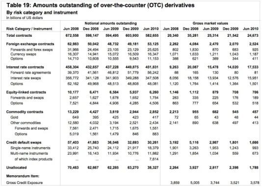
OTC derivatives: notional, mark-to-market and daily variations Table 1 gives an overview of the notional and gross market values of different types of OTC derivatives. We observe that interest rate and foreign exchange instruments account for 85% of the total notional size of the OTC market, while credit default swaps account for around 5%. On the other hand,
Table 1: Amounts outstanding of OTC derivatives. Source: BIS Quarterly Review, December 2010.
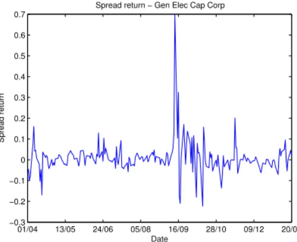
when looking at the daily variation of the mark-to-market values of these instruments - that we approximate by the daily variation of spreads and respectively the swap fixed rate - the picture changes, as shown in Figure 2. Turbulent times like the weeks following the failure of Lehman Brothers on the 15th Sept 2008, showed that the absolute value of the average 5-year CDS spread variation for the high-grade names comprising the CDX index can be several times larger than the absolute value of the variation of the swap fixed rate. Moreover, spreads of institutions belonging to the same sector as a failed institution exhibit particularly large jumps due to cross-sector correlation. Such is the case of General Electric, which is a component of the CDX index within the sector ‘financials’, whose 5-year spread had a 70% jump following the default of Lehman Brothers. Institutions closer in their activity to that of the failed bank, like
other dealer banks, suffered even larger jumps in spreads: the cost of protection for other dealers doubled over a few trading days in the aftermath of Lehman’s default [Brunnermeier, 2009].
As documented in [Cont and Kokholm, 2014], the risk per dollar notional of a CDS exposure is typically 3 or more times higher than the risk per dollar notional for an interest rate swap constract with a similar maturity.
05/08 15/09 −0.1 −0.05 0 0.05 0.1 0.15 Date
Average 5YR spread relative variation over 125 CDX names
Average 5YR spread relative variation over 125 CDX names
(a) Average 5-year CDS spread variations for the CDX.NA.IG index 01/04 13/05 24/06 05/08 16/09 28/10 09/12 20/01 −0.3 −0.2 −0.1 0 0.1 0.2 0.3 0.4 0.5 0.6 0.7 Date Spread return
Spread return − Gen Elec Cap Corp
(b) GE 5-year CDS spread variations
Figure 1: Spread variations for CDS
Concentration in OTC markets Another important empirical observation is the concen-tration of the OTC market. Table 2 extracted from [OCC, 2010] shows the notional positions of the top 5 US dealers on different types of OTC derivatives: forwards, swaps, options and credit.
Rank Holding Assets Total OTC Forwards Swaps Options Credit Company derivatives 1 JPM 2117605 75510099 11806979 49331627 8899046 5472447 2 BAC 2268347 63983932 10287375 43481989 5847866 4366702 3 C 1913902 45151220 6895160 28638854 7071397 2545809 4 GS 911330 43998391 3805327 27391560 8568358 4233146 5 MS 807698 41124050 5458883 27161921 3854976 4648270
Table 2: Notional Amount of Derivative Contracts Top 5 Holding Companies In OTC Deriva-tives December 31, 2010, $ millions. Source: OCC’s Quarterly Report on Bank Trading and Derivatives Activities Second Quarter 2010.
According to this data, the top 5 US dealers alone hold an OTC derivative global mar-ket share of 46%. For credit derivatives in particular, their global market share is 71%. This demonstrates that the credit derivatives market is significantly more concentrated than the other OTC markets. For CDS, a comprehensive analysis of concentration is made in
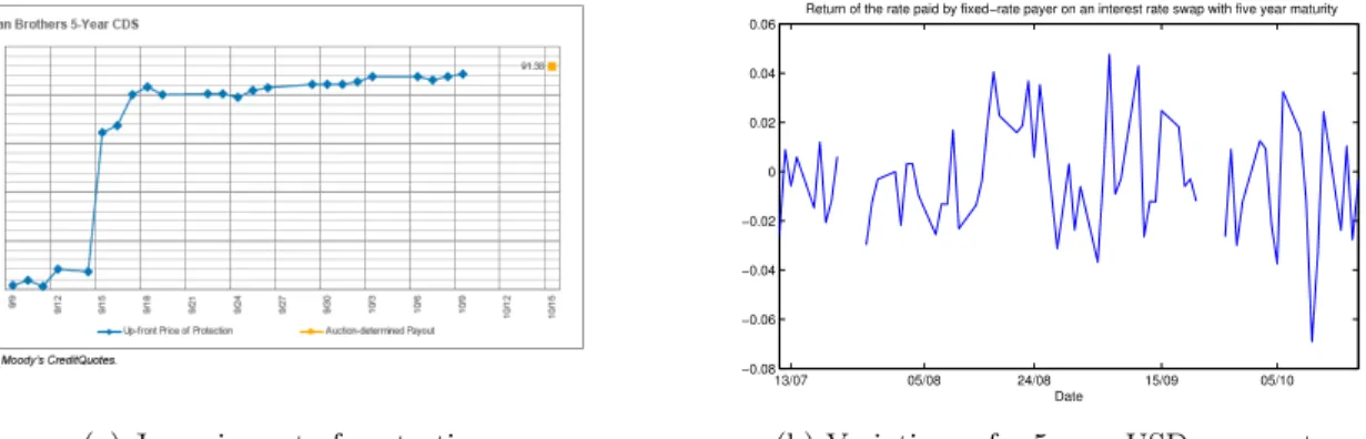
(a) Jump in cost of protection 13/07 05/08 24/08 15/09 05/10 −0.08 −0.06 −0.04 −0.02 0 0.02 0.04 0.06 Date
Return of the rate paid by fixed−rate payer on an interest rate swap with five year maturity
(b) Variations of a 5 year USD swap rate.
Figure 2: Daily variations in OTC derivatives values: IR Swaps vs CDS.
[European Central Bank, 2009]. According to DTCC data, the total notional amounts of out-standing CDSs sold by dealers worldwide, represent over 80% of total protection sold worldwide and a similar percentage is represented by protection bought by dealers. Also, the interdealer network accounts for 75% of total CDS notional. Remark that no precise number of dealers is given in DTCC data, they are defined as “any user that is, or is an affiliate of a user who is, in the business of making markets or dealing in credit derivative products”.
When considering the distribution of the total notional among reference entities, we observe an important concentration on the top underlying names, as shown in Figure 3.
[Peltonen et al., 2014] arrive at a similar conclusion regarding the concentration of the CDS market using a more detailed dataset from a different period.
Although non-credit OTC derivatives have a mark-to-market value one order of magnitude above credit derivatives, CDS may present much larger variations in the mark-to-market values [Cont and Kokholm, 2014] and as a result for large dealers the variation margins for positions on CDS and non-CDS derivatives are comparable.
All these observations plead for distinguishing CDS and credit derivatives from non-credit OTC derivatives (primarily interest rate swaps and other interest rate derivatives) and account-ing for their differences in terms of size, concentration and riskyness in the model.
20 40 60 80 100 120 140 160 180 200 0 1 2 3 4 5 6 7 8 9 10x 10 10
Rank of underlying name
Notional
Gross notional of protection
0 0.5 1 1.5 2 2.5 x 10¹¹ 100 101 102 103 Outstanding CDS Notional Probability Distribution
Distribution of the Outstanding CDS Notional
Figure 3: Concentration on names: 47 % of the total CDS Notional is written of the top 5 names and 76 % on the top 10 names.
accommodating these empirical observations.
3
A network model for contingent OTC exposures
At any time, a snapshot of the OTC market reveals a set of institutions (“banks”) that are interlinked by their mutual claims. We denote by [n] :={1, . . . , n} the set of banks.
We consider a two period model t = 0,1,2. At time 0 banks enter the OTC contracts. At time 1 the payables are revealed. The payables are random variables that depend on the contract specification and the realization of random shocks at time 1. We consider the period t = 1,2 as the period during which the cash flows occur. We denote by small letters the quantities known at time 0 and by capital letters the quantities revealed at time 1. There is no new information arriving after time 1, so the cash flows occurring during the period 1,2 are deterministic functions of the quantities known at time 1.
3.1 Payables and receivables
We denote byX : [n]×[n]→R the matrix of receivables at time 1, assumed anti-symmetric. Fori, j∈[n],Xij+ represents the receivable ofifromj and Xij− represents the payable ofitoj and we haveXij =−Xji. Only one of these payables is due, which means that we account for bilateral netting. DenoteLi the liquidity buffer of bankiat time 13
As argued in Section 2, in case of CDS, variations of their MtM value are more realisti-cally defined as percentages of the outstanding notional. Therefore, we model the matrix of receivablesX using
1. The network of non-CDS contracts. This network’s features are realized at time 0.
3
This is constituted by cash in main currencies or other highly liquid instruments like high-grade government securities. Most importantly it includes the total cash that can be raised on the market by the bank for example using repurchase agreements.
2. r networks of outstanding notional of CDS, where [r] denotes the set of reference entities These networks are realized at time 0.
3. The variations of mark-to-market values of OTC derivatives. These variations are realized at time 1.
In the sequel we approximate the mark-to-market value of a CDS contract by the contract notional times the spread of the reference entity, i.e., for reference entity k ∈[r], mkSk gives the mark-to-market value (from the point of view of the buyer of protection), before netting, of the CDS contracts onk.
Letedenote the gross exposures on non-CDS contracts and (mk)k∈[r]the networks of CDS outstanding notionals for each reference entity. Denote by (∆Sk)k∈[r] and ∆M tM the spread variations and respectively the variation of the MtM values of non-CDS derivatives. The matrix of receivables att= 1 is given by X := (e∆M tM+X k m(k) ∆Sk)−(e∆M tM + X k m(k) ∆Sk)t !+ , (1)
where the operator tdenotes matrix transposition.
A bank is said to befundamentally liquid if, assuming all other banks pay their payables in full, it can meet its payables in full
Li+X j Xij+−X j Xij−=Li+X j Xij ≥0. (2)
It is said to be fundamentally illiquid otherwise.4
If the bank is fundamentally illiquid, it will default on its payment obligations and an illiquidity cascade may emerge.
Assumption 3.1. Upon default, we consider that in the short run recovery rates are 0.
The second assumption is standard in the literature on cascading defaults in financial net-works [Amini et al., 2011].
A bank becomes illiquid due to contagionif its liquidity buffer is such that it depends on its receivables from the other banks in order to meet its own payment obligations. Such a situation can arise for highly ‘leveraged’ banks, i.e. banks that are well hedged and holding little liquidity.
Consider the example of an institution A that buys protection from an institutionB on a reference entitykfor a total notionalm(k). InstitutionB will hedge its exposure to the default of the reference entity by buying protection from an institutionC on the same notional amount as it sold protection on toA, and so on, until reaching an institution Dwhich is a net seller of protection. All the intermediary institutions are well hedged and have little incentive to keep a
4
Such a situation may arise from large jumps in mark-to-market values of net OTC derivatives payables, stemming for example from large correlated jumps in the spreads of reference entities of CDS. Institutions with large unilateral positions are particularly prone to this kind of illiquidity. Nonetheless, our model allows for a bank to become fundamentally illiquid via an exogenous shock like a run by short term creditors.
high liquidity buffer , especially if counterparties have high ratings (i.e. are deemed as having small probability of default). On the other hand, payables may be particulary large following jumps in the spread of the reference entity. If the end net seller of protection defaults, then there is potential of domino effects along the chain of intermediaries.
Definition 3.2(Illiquidity cascade). Starting from the liquidity buffer s at time1, {Li}1≤i≤n,
and the matrix of receivables {Xij}1≤i<j≤n, the illiquidity cascade can be determined as follows
• The set D0 of initially illiquid banks is defined as
D0 ={i∈[n] |Li+
X
j
Xij <0}
• For r ≥1, set Dr = {i∈ [n] | Li+PjXij −Pj∈Dr−1X
+
ij < 0}, the set of institutions
which become illiquid after r iterations.
We obtain an increasing sequence of defaults D0 ⊂ D1,· · · ⊂ Dn−1. The set Dn−1 represents
the final set of illiquid banks.
First, note that the liquidity buffer Land the matrix Xof receivables tend to be negatively correlated. Again, let us take the example of a CDS protection seller. In a first approximation, the jump in the negative position of the seller is given by the jump in the spread of the reference entity. As pointed out by [Cont and Kan, 2011], the spread variation exhibits positive autocorrelation, volatility clustering and heteroscedasticity. Their empirical distribution of the spread variation is heavy tailed. Moreover, empirical data shows that spread variations are correlated across certain classes of reference entities. It follows that a large value for derivatives payables is very likely to occur after a period of increases in spreads, which had the effect of fragilizing the liquidity buffer of the seller. This is a typical example of wrong-way risk, exacerbated if this seller concentrates positions on several correlated reference entities.
Second, one should not ignore that large downward jumps in market values may also cause contagion. In case banks use rehypothecation5, there is no guarantee that a party with negative exposure will receive back its excess collateral in case the (absolute value) of the exposure diminishes. This may cause the party to become illiquid if it is part of an intermediation chain. Whereas the danger of rehypothecation has been pointed out in relation to this kind of collateralization [Singh and Aitken, 2009], one should keep in mind that the risk of over-collateralization incurred by one party is the dual of the risk of under-over-collateralization incurred by the other party.
3.2 A network model for OTC exposures
We now detail the model for exposure matriceseand (m(k))k∈[r]. The construction of the OTC network with vertex set [n] = {1, . . . , n} is centered around the fact that a small subset of these institutions, among the largest and most interconnected, act primarily as intermediaries
5Rehypothecation refers to an institution posting as collateral to its creditors the collateral that it received from its debtors.
between other institutions, so that generally they are counterparties to off-setting contracts. We refer to these institutions as dealers or intermediaries.
The model is based on the following parameters:
• The aggregate gross value of the OTC market (source: BIS);
• The non-credit derivatives market share for the top 10 dealers (source: OCC);
• The credit derivatives market share for the top 10 dealers (source: DTCC);
• The gross CDS protection bought on the top 1000 reference entities (source: DTCC);
• The net CDS protection bought on the top 1000 reference entities (source: DTCC).
3.2.1 A matching model for non-CDS exposures
We detail the construction of the network e of non-CDS exposures using a weighted version of Blanchard’s random graph model [Blanchard et al., 2003]. We assume that we are given a sequence of out degrees (d+i )i∈[n]. Our goal is to construct a networkesuch that for anyi∈[n], d+i represents the sum of the elements on the columni(this has the financial interpretation of the number of banks to which bank iis exposed)
d+i =X j
eij.
We assume that the empirical distribution of the out-degree approximates a power law with tail coefficientγ+(real financial networks have been shown to exhibit these degree distributions [Cont et al., 2013]): Condition 3.3. lim n→∞#{i|d + i =j} ∼jγ ++1 . (3)
In [Blanchard et al., 2003], a random graph is chosen among all graphs that have these out-degrees using a sequential matching: an arbitrary out-going edge will be assigned to a node with probability proportional to the powerα of the node’s out-degree. Forα >0, one obtains positive correlation between in and out-degrees. The main theorem in [Blanchard et al., 2003] states that the marginal distribution of the resulting out-degree approximates a distribution with a Pareto tail with exponentγ−= γα+, provided 1≤α < γ+:
lim n→∞#{i|d − i =j} ∼jγ −+1 .
We now extend this model to account for the heterogeneity of weights. The intuition behind our construction can be given by rephrasing the Pareto principle: 20% of the links carry 80% of the mark-to-market value of non CDS derivatives. Therefore, we will distinguish between two types of links.
• Links of type A represent a percentage a of the total number of links and carry a per-centage a0 of the total mark-to-market value.
• All other links are said to be of typeB.
We can now define the random graph model that we use to model the non-CDS mark-to-market values which is a weighted version of Blanchard’s random graph model [Blanchard et al., 2003].
Definition 3.4 (Heterogeneous exposure network). Let (d+i )i∈[n] be a sequence of out-degrees,
assumed to verify Condition (3.3). For every nodei, itsd+i out-going links are partitioned into
d+,Ai links of type A and d+,Bi links of type B:
d+i =d+,Ai +d+,Bi . (4) We denote mA := Pn i=1d +,A i and by mB := Pi i=1d +,B
i their respective numbers. Denote
FA :Rm
A
+ → [0,1] and FB :Rm
B
+ → [0,1] the joint probability distributions functions for the
weights carried by links of type AandB respectively. The probability distribution functionsFA
and FB are assumed to be invariant under permutation of their arguments (exchangeability).
The graph is generated then as follows:
• Generate the weighted subgraph of links of type A by Blanchard’s algorithm with degree
sequence(d+,Ai )i∈[n] and parameter α >0.
• Draw mA random variables from the joint distribution FA. Assign these exchangeable
variables in arbitrary order to the links of type A.
• Proceed similarly for the links of type B.
The tail coefficientγ+is calibrated to the dealers’ market share in OTC derivatives in Table 2. We let α= 1. The topology of the non-CDS exposure network is governed by the following parameters : γ+= 2, α= 1,a= 5%.
Denoting byT the total gross mark-to-market value of non-CDS derivatives, the exposures are governed by the cumulative distribution functions FA and FB. We generate the weights of type A as the differences of the order statistics of mA i.i.d. random variables, uniformly distributed in the interval [0, a0 ·T]. We take FB as the distribution of mB i.i.d. random variables drawn from the Pareto distribution with tail coefficient γL. The exposure sequence is governed by the following parameters : T = 3.5$tn,a0 = 80%,γL= 1.1.
3.2.2 A multi-layered network model for CDS exposures
We denote by [r] the set of reference entities.6 We denote by [I]⊆[n] the set of intermediaries, which are assumed to be the nodes with the highest connectivity in the network of exposures e.
For each k∈[r], we denote bygross(k) and respectively bynet(k) the aggregate gross and net notional written on the name k. The gross notional represents the sum over all contracts
6
referencing nodek. The net notional represents the sum over all nodes of the net protection sold on namek. Note that the latter sum is equal to the sum over all nodes of the total protection bought on name k. The ratio of the net and gross notional on a name k provides a measure of the average length of intermediation chains of contracts with k as a reference entity. Each intermediation chain links two customers with opposite positions and passes through a number of dealer banks, with zero net position (see Figure 4). We will refer to contracts between dealers as intermediary contracts and to contracts between a customer and a dealer as end contracts.
b i1
. . . il−1
s w w w w
Figure 4: Hedging chain for one CDS contract on reference entityk. The length of the chain isl=bgross(k)net(k) c.
The following algorithm generates an OTC network calibrated to a a given set of
• net and gross CDS notionals (gross(k), net(k))k∈[r]
• market shares for each dealer.
Algorithm 3.5 (Network of notional). Let w the standard notional of a single CDS contract.
For every reference entity k∈[r]:
1. Let bgross(k)net(k) c −1 the number of dealers between two end contracts on reference entity n;
2. Let bnet(k)w c the number of end contracts in which a customer is a buyer of protection;
3. For each pair of nodes i and j, set m(k)ij ←0 the number of contracts on reference entity
k in which isells protection to j;
4. For each contract 1, . . . ,bnet(k)w c, iterate:
• Choose a sequence(b, i1, . . . , ibgross(k)
net(k) c−1
, s)consisting of the end-user acting as buyer
of protection on name k, the intermediary dealer banks and the end-user acting as
seller of protection on name k.
The intermediary i1 is chosen on [I] from the probability distribution p conditioned
on being different from the reference entity k and any subsequent intermediary is
chosen on [I]from probability distribution p conditioned on being different from the
reference entityk and the previous intermediary in the sequence.
The customerbis chosen over the set[n]\[I]and the end-usersis chosen uniformly
over [n]\[I], conditioned on being different from b. The resulting hedging chain is
shown in Figure 4.
For each dealer bank i∈[I] the number of contracts in whichi acts as protection seller is given byP
j∈[n]m (k) ij .
Remark 3.6. An alternative construction could be to consider that each market participants
hedges a proportion ρ < 1 of its exposures. In this case, an initial transaction of notional w
leads to a chain of secondary transactions with notionals ρw, ρ2w, ..., ρl−1w. In this case the
total gross notional along the chain is 2w(1−ρl)/(1−ρ) and the net notional is 2w, so the
parameter ρ can be calibrated to the ratio of net to gross notional, which is (1−ρl)/(1−ρ). 7
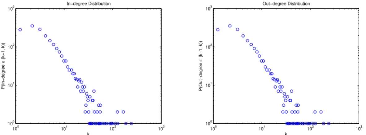
3.3 Calibration results for a sample OTC network
The features of a sample of the random networkeof non-CDS exposures are shown in Figure 5. 100 101 102 103 100 101 102 103 k P(In−degree ∈ [k−1, k)) In−degree Distribution
(a) The distribution of out-degree has a Pareto tail with exponent 2 100 101 102 103 100 101 102 103 k P(Out−degree ∈ [k−1, k)) Out−degree Distribution
(b) The distribution of the in-degree has a Pareto tail with exponent 2
109 1010 1011
10−4
10−3
10−2
k
P(Non CDS Exposure Size > k)
Non CDS Exposure Size Distribution
(c) Cross-sectional distribution of exposures.
1 2 0 5 10 15x 10 12 US Dollar
Concentration of the non−CDS OTC Market Top 10 dealers Remaining institutions
(d) Concentration on the top dealers
Figure 5: Features of the OTC (non-CDS) exposure network.
7
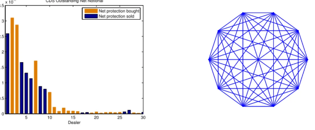
Based on this sample, a CDS network generated from the model of Section 3.2.2 has, by construction, the same features as given by the empirical data: the top five CDS dealers sell protection totaling 65% of the CDS outstanding notional, the top ten sell protection totaling 87 % of the outstanding notional. Also, as shown by Figure 6, the subnet of CDS contracts sold by the top ten dealers to other top ten dealers is a complete network. This network represents in our calibrated sample 76 % of the total outstanding notional.
5 10 15 20 25 30 0 0.5 1 1.5 2 2.5 3 3.5x 10 11 Dealer Net notional
CDS Outstanding Net Notional
Net protection bought Net protection sold
(a) The Dealer structure of the CDS Market : first 10 largest dealers sell/buy 87 % / 88 % of the total CDS Notional
(b) Dealer to dealer network: complete network representing 76 % in terms of outstanding CDS notional
Figure 6: Concentration in the CDS market
The results of the calibration to DTCC data on the net and gross notional sold on the top reference entities are show in Figure 7. Since the top reference entities are not necessarily financial institutions, the notionals of protection sold on nonfinancial names - the data also includes sovereigns - have been aggregated (in Figure 7 the point with the highest notional corresponds aggregates the non-financial reference entities).
109 1010 1011 1012 1013 1014 109 1010 1011 1012 1013 1014 Gross CDS Protection Calibrated Data 108 109 1010 1011 1012 108 109 1010 1011 1012 Net CDS Protection Calibrated Data
Figure 7: Calibration to DTCC Data [DTCC, 2010]
4
Does central clearing of CDS reduce systemic risk?
The purpose of this section is to analyze the impact of central clearing on an OTC network. This network is constructed as a sample of the random network introduced in the previous section. When the complete network is observed at time 0, we may use the resilience indicator to assess the transmission of distress under a stress scenario.
4.1 Resilience to illiquidity cascades in stress scenarios
We now explain the methodology for stress-testing the OTC network: we consider a stress
scenario ω defined by
• a vector of CDS spread variations across reference entities ∆S= (∆Sk(ω))k∈[r],
• the variation of the mark-to-market value of the non-CDS derivatives ∆M tM = ∆M tM(ω),
• liquidity reserves of financial institutions L= (Li(ω))i∈[n].
The matrix of receivables in the stress scenario ω is then given by (1). The magnitude of the illiquidity cascade can be investigated on the network X either directly using simulation. or using the asymptotic analysis given in [Amini et al., 2011], as we now explain.
As in [Amini et al., 2011], we note that contagion takes place primarily along a sub-network defined by ’weak links’ which, in this case, can be understood as ’critical receivables’:
Definition 4.1 (Critical receivables). Let i be a node that does not become fundamentally
illiquid under the stress scenario ω, i.e. Li(ω) +P
jXij(ω)>0. We say that, under the stress
scenario ω, there is a critical cash flow between k and iif
Xik+> Li+X j
i.e. node icannot meet its payables if node k is illiquid. We write in this case
k→c i.
We now definew(i) = #{k∈[n]| k→c i}the number of ’weak links’ ofi, i.e. the number of liquidity inflows the absence of which would renderiilliquid. Ifw(i) = 0 this means the nodei has sufficient liquidity to cover the scenario where any single inflow is cancelled: this should be the case in a ’normal’ regime, and this is indeed the focus of current regulatory requirements on liquidity ratios. Nevertheless, in a stress scenario we can have w(i, ω) > 0 i.e. weak links may appear due to liquidity shocks.
Moreover, we denote by
Ci+= #{j∈[n]s.t. Xij >0},
thein-degreeof a nodei, given by the number of its in-flows, while its out-degreeof a nodeiis
the number of its out-flows
Ci−= #{j∈[n]s.t. Xij <0}.
Clearly we have that the total number of linkages in the system is given by
X
i∈[n]
Ci+ = X i∈[n]
Ci−.
Following [Amini et al., 2012], we consider the following indicator of the network’s resilience to contagion:
Definition 4.2 (Resilience to contagion in a stress scenario). The resilience indicator of the
CDS network in stress scenarioω is defined as
ˆ ν(ω) := 1−P 1 j∈[n]C − j X i∈[n] Ci−w(i, ω). (6)
A key result shown in [Amini et al., 2011] is that a negative value of ˆν(ω) indicates that there exists a large subnetwork of banks strongly interlinked (there is a path from any node to another node) by critical receivables. As such, any default of a node in this subnetwork triggers the illiquidity of the whole subnetworks.
4.2 The stress scenario
Starting from the OTC networks, the matrix of receivables X is determined in our example according to following stress scenario:
• The gross market values of credit default swaps having as a reference entity one of the dealers have an absolute jump equal to 15% of the notional;
• The gross market values of credit default swaps having as a reference entities other finan-cial institution aside dealers, has an absolute jump equal to 10% of the notional;
• The gross market value of credit default swaps on other reference entities has an absolute jump equal to 5% of the notional;
• The gross market value of the other OTC derivatives confounded decreases by 5%.
For any banki, the liquidity buffer at time 0 is assumed to be the minimal liquidity buffer such that no bank has any critical receivables in the event of a jump equal to a percentageγ = 5% of the MtM value of non-CDS derivatives and respectively of the CDS notionals:
`i=γ·( X j eji− X j eij+ max j (eij−eji) +)+ +γ·(X j X k m(k)ji −X j X k m(k)ij ) +γ·max j ( X k m(k)ij −X k m(k)ji )+, (7)
and the liquidity buffer at time 1 is
Li=`i(1−ε),
where ε is an exogenous liquidity shock assumed constant over all banks between time 0 and time 1.
Clearly, since our stress scenario is more severe, critical receivables will appear in the system. We investigate the role of central clearing in mitigating the transmission of distress via these critical receivables, under several clearing configurations. Concerning the CDS, we consider three case studies:
1. The case where CDS are not centrally cleared;
2. The case where CDS are centrally cleared with a set of 20 dealers;
3. The case where CDS are centrally cleared but only a reduced set of 10 dealers have access to the clearing house.
Concerning the other derivatives, in their majority IR derivatives, we compare the following cases:
1. The case without central clearing; 2. The case of a dedicated clearing house; 3. The case of joint clearing with CDS.
Note that the definition of the liquidity buffer given by (7) is independent of any netting across derivative classes. The reason for this is that different cases of clearing strongly affect the netting opportunities, whereas we need precisely a definition of the liquidity that would serve for a common base for comparing these cases.
On the other hand, the liquidity buffer of the clearing houses is defined by taking into account the possibilities of netting across derivative classes. Also, more precaution is taken: not only the clearing house is not allowed to have critical receivables (which implies that the CCP withstands the default of any of its members), but it must withstand the default of the two members to which it has the largest exposure. Note also that the cash inflows of any
clearing house equal its outflows. So, for a clearing house c, the liquidity buffer at t = 0 is given by `c= 2·γ·max j (e(c, j)−e(j, c) + X k m(k)(i, c)−X k m(k)(c, i))+, (8) and we assume no exogenous liquidity shock for the clearing houses between time 0 and time 1
Lc=`c.
4.3 Simulation results
Using the stress scenarios considered in the previous section, we now assess the impact of central clearing on the sample network presented in the previous section. We will compute the resilience indicator given by Definition 4.2. Figure 8 shows the size of the illiquidity cascade in the stress scenario as a function of a varying exogenous liquidity shockε. Recall that for every banki, the liquidity shock is defined as a fixed percentage of the liquidity buffer`i given in (7) and this percentage is constant over all banks. In all cases, we relate the size of the illiquidity cascade to the resilience indicator.
These results show that, as in [Amini et al., 2012], as the resilience indicator becomes neg-ative a ’phase transition’ occurs: the sub-network of critical receivables acquires a giant com-ponent along which contagion can take place, exposing the system to a possible large scale illiquidity cascade. Since the resilience indicator indicates the tipping point where the onset of contagion occurs, we can use it to assess the effect of central clearing on the mitigation of systemic risk.
The results show, that in absence of central clearing of the other classes of derivatives, CDS clearing does not impede the phase transition. It is the large size of the jump in IR swaps (recall the stress scenarios consider a jump equal to 5 % of the MtM value of IR swaps) that plays a dominating role here and the system cannot withstand even a small liquidity shock. However, when IR swaps are centrally cleared, CDS clearing has an important impact on impeding the phase transition. Both in the case where the IR swaps are cleared in a dedicated CH and the case of joint clearing, when a CH for CDS with the top 20 members is introduced, the phase transition occurs for a significantly larger liquidity shock. Without CDS clearing, a liquidity shock of 3% induces a phase transition. With CDS clearing with 20 members, the onset of contagion occurs when the liquidity shock reaches 12%.
We observe that the benefits of central clearing decrease when less members are allowed in the CH. We can explain this in the following way. Recall that the CDS network is constructed by introducing the intermediation chains. Introducing a CCP compresses the intermediation chains consisting exclusively of clearing members. For example if a intermediation chain has length 10 and all intermediaries are members of the CH, then this chain will have length two after compression. On the other hand it suffices for only one of the intermediaries to be a non-member of the CH for the benefits to decrease. It follows that not just the size of notional of protection sold/bought should be a criterion to allow a member in the clearing house, but it should also be accounted for the number of intermediation chains passing through this node. Here a dealer is considered significant if it has both an important market share but more importantly, is present as an intermediary in a large number of the intermediation chains.
0.020 0.04 0.06 0.08 0.1 0.12 0.14 0.16 200 400 600 800 1000 1200 1400 1600 1800 2000 Liquidity shock
Number of illiquid banks
Number of illiquid banks − Without IR CH
Without CDS CH CDS CH (top 20 dealers) CDS CH (top 10 dealers) (a) 0.02 0.04 0.06 0.08 0.1 0.12 0.14 0.16 −0.8 −0.6 −0.4 −0.2 0 0.2 0.4 0.6 Liquidity shock
Resilience to illiquidty measure
Resilience to illiquidity measure − Without IR CH Without CDS CH CDS CH (top 20 dealers) CDS CH (top 10 dealers) (b) 0.020 0.04 0.06 0.08 0.1 0.12 0.14 0.16 200 400 600 800 1000 1200 1400 1600 1800 2000 Liquidity shock
Number of illiquid banks
Number of illiquid banks − With Dedicated IR CH
Without CDS CH CDS CH (top 20 dealers) CDS CH (top 10 dealers) (c) 0.02 0.04 0.06 0.08 0.1 0.12 0.14 0.16 −0.8 −0.6 −0.4 −0.2 0 0.2 0.4 0.6 Liquidity shock
Resilience to illiquidty measure
Resilience to illiquidity measure − With Dedicated IR CH Without CDS CH CDS CH (top 20 dealers) CDS CH (top 10 dealers) (d) 0.020 0.04 0.06 0.08 0.1 0.12 0.14 0.16 200 400 600 800 1000 1200 1400 1600 1800 2000 Liquidity shock
Number of illiquid banks
Number of illiquid banks − With IR/CDS CH
Without CDS CH CDS CH (top 20 dealers) CDS CH (top 10 dealers) (e) 0.02 0.04 0.06 0.08 0.1 0.12 0.14 0.16 −0.8 −0.6 −0.4 −0.2 0 0.2 0.4 0.6 Liquidity shock
Resilience to illiquidty measure
Resilience to illiquidity measure − With IR/CDS CH Without CDS CH CDS CH (top 20 dealers) CDS CH (top 10 dealers)
(f)
5
Conclusions
We have introduced a multi-layered network model, with a core-periphery structure, for study-ing illiquidity contagion in OTC derivatives markets. Our model accounts for the heterogeneity in gross and net notional exposures and market share of market participants in each asset class, as well as the presence of intermediation chains which characterize OTC markets. In such a setting, liquidity shocks may generate contagion along an intermediation chain.
Our model provides a framework for studying the magnitude and dynamics of illiquidity cascades in OTC markets, in stress scenarios formulated in terms of liquidity shocks and vari-ations of the contracts’ mark-to-market value. This analysis may be done using simulation of cash flows in a stress scenario, but also using a simulation-free approach based on insights from asymptotic analysis of large networks [Amini et al., 2011]. We introduce an indicator of the resilience of the network to liquidity shocks that highlights the role of ‘critical receivables’ i.e. receivables on which an intermediary depends to meet its own short-term obligations, and show that this indicators allows to detect phase transitions, i.e., the tipping point when the liquidity shock generates large-scale contagion in the financial system.
Finally, we have used this framework allows to analyze the impact of CDS clearing on systemic risk.
Our analysis shows that, while in absence of a clearing facility for interest rate swaps, an additional clearing facility for CDS does not appear to enhance financial stability, when interest rate derivatives (mainly swaps) are centrally cleared –as is currently the case– and under adequate capitalization, a CDS clearinghouse can contribute significantly to financial stability by enhancing the resilience of the OTC network to large liquidity shocks, provided all significant dealers are members of the clearing house. However, the impact of the CCP on network stability is weakened if some major intermediairies are not clearing members.
Our study provides a framework for studying the impact of central clearing of OTC deriva-tives on systemic risk and is potentially applicable to other data sets and products.
References
[Amini et al., 2011] Amini, H., Cont, R., and Minca, A. (2011). Resilience to Contagion in Financial Networks. To appear in: Mathematical Finance, http://dx.doi.org/10.1111/ mafi.12051.
[Amini et al., 2012] Amini, H., Cont, R., and Minca, A. (2012). Stress testing the resilience of financial networks.International Journal of Theoretical and Applied Finance, 15(1):1250006– 1250026.
[Amini et al., 2013] Amini, H., Filipovic, D., and Minca, A. (2013). Systemic risk with central counterparty clearing. Swiss Finance Institute Research Paper No. 13-34. http: // ssrn. com/ abstract= 2275376.
[Blanchard et al., 2003] Blanchard, P., Chang, C.-H., and Kr¨uger, T. (2003). Epidemic thresh-olds on scale-free graphs: the interplay between exponent and preferential choice. Annales
[Brunnermeier, 2009] Brunnermeier, M. K. (2009). Deciphering the liquidity and credit crunch 2007-2008. Journal of Economic Perspectives, 23(1):77–100.
[Cont, 2010] Cont, R. (2010). Credit default swaps and financial stability. Financial Stability
Review (Banque de France), 14:35–43.
[Cont and Kan, 2011] Cont, R. and Kan, Y. H. (2011). Statistical Modeling of Credit Default Swap Portfolios. http: // ssrn. com/ abstract= 1771862.
[Cont and Kokholm, 2014] Cont, R. and Kokholm, T. (2014). Central clearing of otc deriva-tives: bilateral vs multilateral netting. Statistics and Risk Modeling, 31(1):3–22.
[Cont et al., 2013] Cont, R., Moussa, A., and Santos, E. B. (2013). Network structure and systemic risk in banking systems. In Fouque, J.-P. and Langsam, J., editors, Handbook of
systemic risk. Cambridge University Press.
[DTCC, 2010] DTCC (2010). Trade information warehouse data. http://www.dtcc.com/ products/derivserv/data/index.php.
[Duffie et al., 2014] Duffie, D., Scheicher, M., and Vuillemey, G. (2014). Central clearing and collateral demand. Working Paper.
[Duffie and Zhu, 2011] Duffie, D. and Zhu, H. (2011). Does a central clearing counterparty reduce counterparty risk? Review of Asset Pricing Studies, 1:74–95.
[ECB, 2009] ECB (2009). Credit default swaps and counterparty risk. Technical report, Eu-ropean Central Bank.
[European Central Bank, 2009] European Central Bank (2009). Credit default swaps and coun-terparty risk.
[Farboodi, 2014] Farboodi, M. (2014). Intermediation and voluntary exposure to counterparty risk. Working paper, University of Chicago.
[Gai and Kapadia, 2010] Gai, P. and Kapadia, S. (2010). Contagion in Financial Networks.
Proceedings of the Royal Society A, 466(2120):2401–2423.
[Glode and Opp, 2013] Glode, V. and Opp, C. (2013). Adverse selection and intermediation chains.
[Heller and Vause, 2012] Heller, D. and Vause, N. (2012). Collateral requirements for manda-tory central clearing of over-the-counter derivatives. BIS Working Paper 373, Bank for International Settlements.
[ISDA, 2010] ISDA (2010). Market review of OTC derivative bilateral collateralization prac-tices. http://www.isda.org/c_and_a/pdf/ISDA-Margin-Survey-2010.pdf.
[Macroeconomic Assessment Group on Derivatives (MAGD), 2013] Macroeconomic Assess-ment Group on Derivatives (MAGD) (2013). Macroeconomic impact assessAssess-ment of OTC derivatives regulatory reforms. Technical report, Bank for International Settlements.
[OCC, 2010] OCC (2010). OCC’s quarterly report on bank trading and derivatives activities. Second Quarter.
[Peltonen et al., 2014] Peltonen, T. A., Scheicher, M., and Vuillemey, G. (2014). The network structure of the CDS market and its determinants.Journal of Financial Stability, 13:118–133. [Sidanius and Zikes, 2012] Sidanius, C. and Zikes, F. (2012). OTC derivatives reform and
collateral demand impact. Financial Stability Paper 18, Bank of England.
[Singh and Aitken, 2009] Singh, M. and Aitken, J. (2009). Deleveraging after Lehman – Evi-dence from Reduced Rehypothecation. SSRN eLibrary.
[Stulz, 2010] Stulz, R. M. (2010). Credit Default Swaps and the Credit Crisis. Journal of
Economic Perspectives, 24(1):73–92.
[Watts, 2002] Watts, D. J. (2002). A simple model of global cascades on random networks.
Proceedings of the National Academy of Sciences of the USA, 99(9):5766–5771.
[Zawadowski, 2013] Zawadowski, A. (2013). Entangled financial systems. Review of Financial

![Figure 7: Calibration to DTCC Data [DTCC, 2010]](https://thumb-us.123doks.com/thumbv2/123dok_us/623396.2574857/17.918.126.759.156.415/figure-calibration-to-dtcc-data-dtcc.webp)
