Student Portfolios and the College Admissions Problem
(Article begins on next page)
The Harvard community has made this article openly available.
Please share
how this access benefits you. Your story matters.
Citation
Chade, H., G. Lewis, and L. Smith. 2014. “Student Portfolios and
the College Admissions Problem.” The Review of Economic
Studies (February 17).
Published Version
doi:10.1093/restud/rdu003
Accessed
February 19, 2015 4:09:00 PM EST
Citable Link
http://nrs.harvard.edu/urn-3:HUL.InstRepos:12363836
Terms of Use
This article was downloaded from Harvard University's DASH
repository, and is made available under the terms and conditions
applicable to Open Access Policy Articles, as set forth at
http://nrs.harvard.edu/urn-3:HUL.InstRepos:dash.current.terms-of-use#OAP
Student Portfolios and the
College Admissions Problem
∗
Hector Chade
†Gregory Lewis
‡Lones Smith
§First version: July 2003
This version: January 24, 2014
Abstract
We develop a decentralized Bayesian model of college admissions with two ranked colleges, heterogeneous students and two realistic match frictions: students find it costly to apply to college, and college evaluations of their applications are uncertain. Students thus face a portfolio choice problem in their application decision, while colleges choose admissions standards that act like market-clearing prices. Enrollment at each college is affected by the standards at the other college through student portfolio reallocation. In equilibrium, student-college sorting may fail: weaker students sometimes apply more aggressively, and the weaker college might impose higher standards. Applying our framework, we analyze affirmative action, showing how it induces minority applicants to construct their application portfolios as if they were majority students of higher caliber.
∗Earlier versions were called “The College Admissions Problem with Uncertainty” and “A Supply
and Demand Model of the College Admissions Problem”. We would like to thank Philipp Kircher (Co-Editor) and three anonymous referees for their helpful comments and suggestions. Greg Lewis and Lones Smith are grateful for the financial support of the National Science Foundation. We have benefited from seminars at BU, UCLA, Georgetown, HBS, the 2006 Two-Sided Matching Conference (Bonn), 2006 SED (Vancouver), 2006 Latin American Econometric Society Meetings (Mexico City), and 2007 American Econometric Society Meetings (New Orleans), Iowa State, Harvard/MIT, the 2009 Atlanta NBER Conference, and Concordia. Parag Pathak and Philipp Kircher provided useful discussions of our paper. We are also grateful to John Bound and Brad Hershbein for providing us with student college applications data.
†Arizona State University, Department of Economics, Tempe, AZ 85287. ‡Harvard University, Department of Economics, Cambridge, MA 02138. §University of Wisconsin, Department of Economics, Madison, WI 53706.
1
Introduction
The college admissions process has lately been the object of much scrutiny, both from academics and in the popular press. This interest owes in part to the competitive nature of college admissions. Schools set admissions standards to attract the best students, and students in turn respond most judiciously in making their application decisions. This paper examines the joint behavior of students and colleges in equilibrium.
We introduce an equilibrium model of college admissions that analyzes the impact of two previously unexplored frictions in the application process: students find it costly to apply to college, and college evaluations of their applications is uncertain. As evidence of the noise in the process, observe that admissions rates are well below 50% at the most selective colleges, and below 75% at the median 4 year college.1 This uncertainty
prevailsconditional on the SAT. Even applicants with perfect SAT scores have no better than a 50% chance of getting into schools like Harvard, MIT and Princeton (Avery, Glickman, Hoxby, and Metrick, 2004). So it is not surprising that most applicants construct thoughtful portfolios that include both “safety” and “stretch” schools.
Despite this uncertainty, the costly nature of applications substantially limits the number of applications sent — three for the median student.2 A fast growing empirical literature confirms the impact of this friction: for instance, Pallais (2009) finds that when the ACT allowed students to send an extra free application, 20% of ACT test-takers took advantage of this option.3 Small costs can have large effects on application
behavior because the marginal benefit of applying falls geometrically in the number of applications. A student applying to identical four-year colleges with a typical 75% acceptance rate sees the marginal benefit to her 5th application scaled by 4−4 = 1/256:
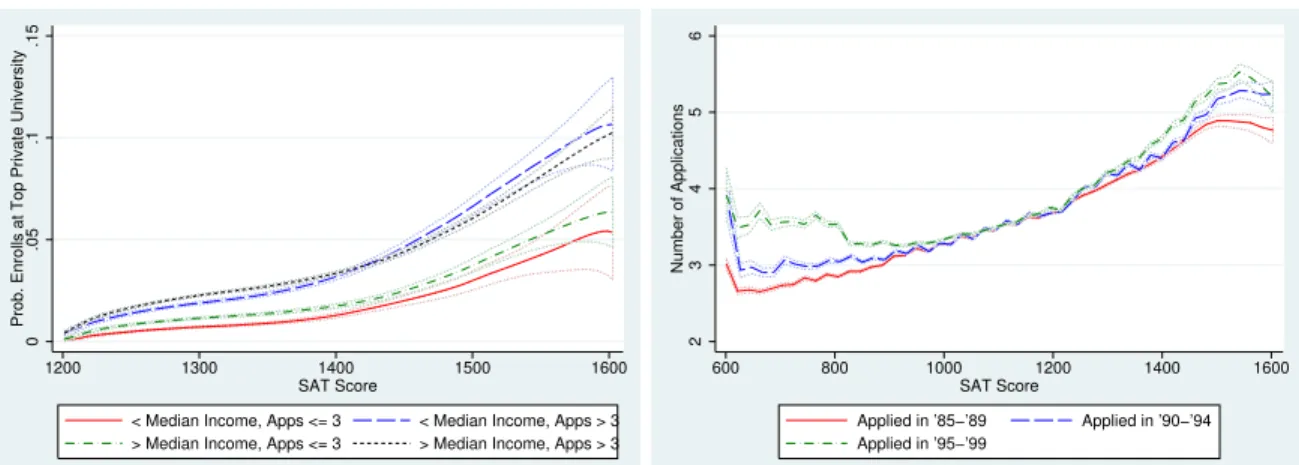
Even if attending college this year is worth $20000, the marginal benefit is only $59. Figure 1 illustrates some motivating patterns in the application data. The left panel demonstrates the importance of the application frictions — for the chance of matric-ulating at a private elite school is significantly higher for students who apply widely.4 The right panel plots the average number of applications as a function of the SAT score,
1Source: Table 329, Digest of Education Statistics, National Center for Education Statistics. 2Source: Higher Education Research Institute (HERI), using a large nationally representative survey
of college freshman since 1966 (data also used to construct Figure 1; see online appendix for details).
3Steinberg (2010) reported that colleges who waived application fees saw applications skyrocket. 4Avery and Kane (2004) study a Boston program giving low-income students advice on how/where to
apply; these students matriculated at a higher rate than comparable students elsewhere. Similar results have later been found in field experiments where students received application help: see Bettinger, Long, Oreopoulos, and Sanbonmatsu (2009) and Carrell and Sacerdote (2012).
0
.05
.1
.15
Prob. Enrolls at Top Private University
1200 1300 1400 1500 1600 SAT Score
< Median Income, Apps <= 3 < Median Income, Apps > 3 > Median Income, Apps <= 3 > Median Income, Apps > 3
2 3 4 5 6 Number of Applications 600 800 1000 1200 1400 1600 SAT Score Applied in ’85−’89 Applied in ’90−’94 Applied in ’95−’99
Figure 1: Applications and Matriculation by SAT.The left panel shows the chance of matriculating at a top private university, by number of applications and household income. The right panel shows the estimated relationship between SAT score and number of applications. Estimation is by local linear regression; 95% confidence intervals are shown as dotted lines.
small but larger than one consistent with our two frictions.5
Any model that focuses on these two frictions — costly portfolio choices with incom-plete information — must diverge from the approach of the centralized college matching literature (Gale and Shapley, 1962), for it expressly sidesteps such matching frictions. Rather, we analyze an entirely decentralized model that parallels the actual process. It affords sharp conclusions about two key decision margins: how colleges set admission standards and how students formulate their application portfolios.
We assume a heterogeneous population of students, and two ranked colleges — one better and one worse, respectively, called 1 and 2. Like the decentralized model of Avery and Levin (2010), there is a continuum of students; this avoids colleges facing aggregate uncertainty — otherwise, wait-listing is needed, for instance.6 Colleges seek to fill their
capacity with the best students possible, but student calibers are only imperfectly ob-served. The tandem of costly applications and yet noisy evaluations feeds the intriguing conflict at the heart of the student choice problem: shoot for the Ivy League, settle for the local state school, or apply to both. As we shall see, our paper formalizes the critical roles played by stretch and safety schools. Meanwhile, college enrollments are
5Admissions rates fall rapidly as college rank rises. So larger portfolios are particularly valuable for
high SAT students applying to top-tier colleges, consistent with the right panel of Figure 1.
6See Che and Koh (2013) for a college admissions model with aggregate uncertainty. We also
omit many real-world elements like financial aid and peer effects, but these are typically ruled out in centralized matching models too. In a recent paper, Azevedo and Leshno (2012) assume a continuum of students in a centralized paper in the spirit of Gale and Shapley (1962), and find that it affords a characterization of equilibrium in terms of supply and demand — one of our observations too.
interdependent, since the students’ portfolios depend on the joint college admissions standards, and students accepted at the better college will not attend the lesser one. This asymmetric interdependence leads to many surprising results.
Central to our paper is a theorem characterizing how student acceptance chances at the colleges covary with student caliber. We deduce that as a student’s caliber rises, the ratio of his admission chances at college 1 to college 2 rises monotonically. We are thus able to solve the equilibrium in three stages, first deducing how acceptance chances translate into application portfolios, and then seeing how portfolio choices across student calibers relate, for any pair of college admission standards; finally, we compute the derived demand for college slots. We analyze the equilibrium of the induced admissions standards game among colleges through the lens of supply and demand: When a college raises its standards, its enrollment falls both because fewer students make the cut — the standards effect — and fewer will apply ex ante — the portfolio effect. Treating admissions standards as prices, these effects reinforce each other. In equilibrium, we uncover a “law of demand”, in which a college’s enrollment falls in its standard. The portfolio effect increases the elasticity of this demand curve.
Analogous to Bertrand competition with differentiated products, colleges will choose admissions standards to fill their desired enrollment, taking rival standards and the student portfolios as given. An equilibrium occurs when both markets clear and stu-dents behave optimally. The model frictions yield some novel comparative statics. For instance, the admissions standards at both colleges fall if college 2 raises its capacity, while lower application costs at either school increase the admissions standards at the better college. We will argue that our equilibrium framework rationalizes the pattern of changing college standards and admission rates recently documented by Hoxby (2009).
In a major thrust of the paper, we ask whether sorting occurs in equilibrium: First,
do the better students apply more “aggressively”? Precisely, the best students apply just to college 1; weaker students insure by applying to both colleges; even weaker ones apply just to college 2; and finally, the weakest apply nowhere. Such an application pattern rationalizes the general rise and fall that we observe in the right panel of Figure 1. Second,does the better college impose higher admissions standards? The answer to this question is no when the lesser college is sufficiently small, for by our “law of demand”, college 2 continues to raise its standards as its capacity falls. Failures of student sorting are more subtle: The willingness of students either to (i) gamble on a stretch school or (ii) insure themselves with a safety school may not be monotone in their types. Conversely,
all equilibria entail sorting when the colleges differ sufficiently in quality and the lower ranked school is not too small. All told, sorting proves elusive with frictions.7 The college
sorting failures that we identify have problematic implications for rankings based on the characteristics of matriculants, such as their SAT scores: Colleges that substantially increase their capacity are penalized, since they must lower their admission standards.
This paper takes very seriously the uncertainty that clouds the student admission process. Students apply to colleges, perhaps knowing their types, or perhaps ignorant of them. Equally well, colleges evaluate students trying to gauge the future stars, and often do not succeed. The best framework for analyzing this world therefore involves two-sided incomplete information. In fact, we later formulate such a richer Bayesian model, and argue that its predictions are well-approximated by ours where students know their types, and colleges observe noisy signals. The sorting failures we claim, as well as the positive theory of how students and colleges react, are in fact robust findings. We conclude the paper with a topical foray into “affirmative action” for in-state applicants, or other preferred applicant groups. We show that colleges impose different admissions standards so as to equate the “shadow values” of applicants from different groups — a form of third degree price discrimination. This, in turn, affects how students behave: in a simple case, lower caliber applicants of a favored group behave as if they were higher caliber applicants from a non-favored group. This is consistent with the reduction in less-qualified minority applications to selective public schools after the end of affirmative action in California and Texas, documented in Card and Krueger (2005).
2
The Model
A. An Overview. The paper introduces three key features — heterogeneous students, portfolio choices with unit application costs, and noisy evaluations by colleges. We impose little additional structure. For instance, we ignore the important and realistic consideration of heterogeneous student preferences over colleges, as well as peer effects. A central feature of our analysis is modeling college portfolio applications. Student choice is trivial if it is costless, and in practice, such costs can be quite high. Indeed, the
7This adds to the literature on decentralized frictional matching — e.g., Shimer and Smith (2000),
Smith (2006), Chade (2006), and Anderson and Smith (2010). The student portfolio problem in the model is a special case of Chade and Smith (2006). In this sense, our paper also contributes to the directed search literature. See Burdett and Judd (1983), Burdett, Shi, and Wright (2001), Albrecht, Gautier, and Vroman (2003) and Kircher and Galenianos (2006)).
sole purpose of the Common Application is to lower the cost of multiple applications.8 Next, we assume noisy signals of student calibers. This informational friction cre-ates uncertainty for students, and a Bayesian filtering problem for colleges. It captures the difficulty faced by market participants, with students choosing “safety schools” and “stretch schools”, and colleges trying to infer the best students from noisy signals. With-out noise, sorting would be trivial: Better students would apply and be admitted to better colleges, for their caliber would be correctly inferred and they would be accepted. We also make two other key modeling choices. First, we assume just two colleges, for the sake of tractability. But as we argue in the conclusion, this is the most parsimonious framework that captures all of our key findings. We also fix the capacity of the two colleges. This is defensible in the short run, and so it is best to interpret our model as focusing on the “short run” analysis of college admissions. We explore the simultaneous game in which students apply to college, and colleges decide whom to admit.9
In the interest of tractability, our analysis assumes that the colleges’ evaluations of students are conditionally independent. This captures the case where students are apprised of all variables (such as the ACT/SAT or their GPA) common to their appli-cations before applying to college. Students are uncertain as to how these idiosyncratic elements such as college-specific essays and interviews will be evaluated, but believe that the resulting signals are conditionally independent across colleges. We revisit this restriction in Section 6, and argue that our main results on sorting are robust, and that we have analyzed a representative case.
B. The Model. There are two colleges 1 and 2 with capacities κ1 and κ2, and a
unit mass of students withcalibers xwhose distribution has a positive density f(x) over [0,∞). Non-triviality demands that college capacity be insufficient for all students, as
κ1 +κ2 < 1. To avoid many subscripts, we shall almost always assume that students
pay a separate but common application cost c > 0 for the two colleges. All students prefer college 1. Everyone receives payoff v > 0 for attending college 1, u∈ (0, v) for college 2, and zero payoff for not attending college. Students maximize expected college
8This general application form is used by almost 400 colleges, and simplifies college applications. It
eliminates idiosyncratic college requirements, but retains separate college application fees.
9Epple, Romano, and Sieg (2006) analyze an equilibrium model that includes tuition as a choice
variable, price discrimination, peer effects, and students that differ in ability and income. Under single crossing conditions, they obtain positive sorting on ability for each income level. Their model, however, does not include costly applications or noise, thus precluding the portfolio effects we focus on and their implications for sorting. While we do not allow colleges to choose their tuition levels, we do not ignore the role of tuition, for one can simply interpret the benefits of attending college as net benefits.
payoff less application costs. Colleges maximize the total caliber of their student bodies subject to capacity constraints.
Students know their caliber, and colleges do not. Colleges 1 and 2 each just ob-serves a noisy conditionally independent signal of each applicant’s caliber. In particular, they do not know where else students have applied. Signals σ are drawn from a condi-tional density function g(σ|x) on a subinterval of R, with cdf G(σ|x). We assume that
g(σ|x) is continuous and obeys the strict monotone likelihood ratio property (MLRP). Sog(τ|x)/g(σ|x) is increasing in the student’s typex for all signals τ > σ.
Students apply simultaneously to either, both, or neither college, choosing for each caliber x, a college application menu S(x) in {∅,{1},{2},{1,2}}. Colleges choose the set of acceptable student signals. They intuitively should use admission standards to maximize their objective functions, so that college i admits students above a threshold signalσi. Appendix A.1 proves this given the MLRP property — despite anacceptance curse that college 2 faces (as it may accept a reject of college 1).
For a fixed admission standard, we want to ensure that very high quality students are almost never rejected, and very poor students are almost always rejected. For this, we assume that for a fixed signal σ, we have G(σ|x) → 0 as x → ∞ and G(σ|x) → 1 as x → 0. For instance, exponentially distributed signals have this property G(σ|x) = 1−e−σ/x. More generally, this obtains for signals drawn from any “location family”, in which the conditional cdf of signals σ is given by G((σ−x)/µ), for any smooth cdf G
and µ >0 — e.g. normal, logistic, Cauchy, or uniformly distributed signals. The strict
MLRP then holds if the density is strictly log-concave, i.e., logG0 is strictly concave.
C. Equilibrium. We consider a simultaneous move game by colleges and students. This yields the same equilibrium prediction as when students move first, as they are atomless.10 An equilibrium is a triple (S∗(·), σ∗
1, σ ∗
2) such that:
(a) Given (σ∗1, σ∗2), S∗(x) is an optimal college application portfolio for each x, (b) Given (S∗(·), σ∗j), college i’s payoff is maximized by admissions standard σ∗i.
We also wish to preclude trivial equilibria in our model in which one or both colleges reject everybody with a very high admissions threshold and students do not apply there.
10See Appendix A.2. Alternatively, colleges could move first, committing to an admission standard.
This is arguably not the case, but regardless, it too yields the same equilibrium properties until we study affirmative action (proof omitted). In the interests of a unified treatment throughout the paper, we proceed in the simultaneous move world.
A robust equilibrium also requires that any college that expects to have excess capacity set the lowest admissions threshold. Sinceκ1+κ2<1, both colleges will have applicants.
In a robust sorting equilibrium, colleges’ and students’ strategies aremonotone. This means that the better college is more selective (σ∗1 > σ∗2) and higher caliber students are increasingly aggressive in their portfolio choice: The weakest apply nowhere; better students apply to the “easier” college 2; even better ones “gamble” by applying also to college 1; the next tier up applies to college 1 while shooting an “insurance” application to college 2; finally, the top students confidently just apply to college 1. Monotone strategies ensure the intuitive result that the distribution of student calibers at college 1 first-order stochastically dominates that of college 2 (see Claim 3 in Appendix A.7), so that all top student quantiles are larger at college 1. This is the most compelling notion of student sorting in our environment with noise (Chade, 2006).
Our concern with a robust sorting equilibrium may be motivated on efficiency grounds. If there are complementarities between student caliber and college quality, so that wel-fare is maximized by assigning the best students to the best colleges, any decentralized matching system must necessarily satisfy sorting to be (constrained) efficient. Since formalizing this idea would add notation and offer little additional insight, we have ab-stracted from these normative issues and focused on the positive analysis of the model.
D. Common versus Private Values. Notice that in our model colleges care about the true caliber of a student and not about the signal per se. In other words, the model exhibits common values on the side of the colleges. Appendix A.1 shows colleges behave in exactly the same way if they do not care about caliber but care only about the signal i.e. the private values case. In this interpretation, students differ in their observables x
(known to both students and colleges), and also in their “fit” for each collegei (known only to the college). College payoffs depend on both observables and fit through the signalσi ≡σi(x, i). Until the affirmative action application in Section 7, all the results
apply to the private values case as well, albeit with a different interpretation.
3
Equilibrium Analysis for Students
3.1
The Student Optimization Problem
We begin by solving for the optimal college application set for a given pair of admission chances at the two colleges. Consider the portfolio choice problem for a student with
admission chances 0 ≤ α1, α2 ≤ 1. The expected payoff of applying to both colleges
is α1v + (1−α1)α2u. The marginal benefit M Bij of adding college i to a portfolio of
college j is then:
M B21 ≡ [α1v+ (1−α1)α2u]−α1v = (1−α1)α2u (1)
M B12 ≡ [α1v+ (1−α1)α2u]−α2u=α1(v−α2u) (2)
The optimal application strategy is then given by the following rule: (a) Apply nowhere if costs are prohibitive: c > α1v and c > α2u.
(b) Apply just to college 1, if it beats applying just to college 2 (α1v ≥ α2u), and
nowhere (α1v ≥c), and to both colleges (M B21 < c, i.e. adding college 2 is worse).
(c) Apply just to college 2, if it beats applying just to college 1 (α2u ≥ α1v), and
nowhere (α2u≥c), and to both colleges (M B12< c, i.e. adding college 1 is worse).
(d) Apply to both colleges if this beats applying just to college 1 (M B21 ≥ c), and
just to college 2 (M B12 ≥c), for then, these solo application options respectively
beat applying to nowhere, as α1v > M B12≥c and α2u > M B21≥c by (1)–(2).
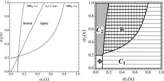
This optimization problem admits an illuminating and rigorous graphical analysis. The left panel of Figure 2 depicts three critical curves: M B21 =c, M B12 =c,α1v =α2u.
All three curves share a crossing point, since M B21 =M B12, when α1v =α2u.
Cases (a)–(d) partition the unit square into (α1, α2) regions corresponding to the
portfolio choices (a)–(d), denoted Φ, C2, B, C1, shaded in the right panel of Figure 2.
This summarizes the portfolio choice of a student with any admissions chances (α1, α2).
In the marginal improvement algorithm of Chade and Smith (2006), a student first decides whether she should apply anywhere. If so, she asks which college is the best singleton. In Figure 2 at the left, college 1 is best right of the line α1v = α2u, and
college 2 is best left of it. Next, she asks whether she should apply anywhere else. Intuitively, there are two distinct reasons for applying to both colleges that we can now parse: Either college 1 is a stretch school — i.e., a gamble, added as a lower-chance higher payoff option — or college 2 is asafety school, added for insurance. In Figure 2, these are the parts of region B above and below the line α1v =α2u, respectively.
The choice regions obey some natural comparative statics. The application region
0.0 0.2 0.4 0.6 0.8 1.0 0.0 0.2 0.4 0.6 0.8 1.0 Α1HxL Α 2 H x L MB12=c Α1v= Α2u MB21=c Safety Stretch 0.0 0.2 0.4 0.6 0.8 1.0 0.0 0.2 0.4 0.6 0.8 1.0 Α1HxL Α 2 H x L
C
1F
C
2B
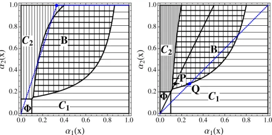
Figure 2: Optimal Decision Regions. The left panel depicts (i) a dashed box, inside which applying anywhere is dominated; (ii) the indifference line for solo applications to col-leges 1 and 2; and (iii) the marginal benefit curves M B12 = c and M B21 = c for adding
colleges 1 or 2. The right panel shows the optimal application regions. A student in the blank region Φdoes not apply to college. Heapplies to college 2 only in the vertical shaded regionC2;
to both collegesin the hashed regionB, andto college 1 onlyin the horizontal shaded regionC1.
region B expands rightwards in the college 2 payoff u, and leftwards in the college 1 payoff v. In particular, if a student enjoys fixed acceptance rates at the two colleges, a college grows less attractive as the payoff of its rival rises. Also, as the application costc
rises, the joint application region B shrinks and the empty set Φ grows.
Although outside our model, let us briefly consider non-linear costs — for instance, the second application costs may be less than c, possibly due to some duplication of forms, essays, etc. We analyze this in the online appendix, and show that region B is bigger and the remaining regions smaller than with constant costs. Interestingly, some types who would send no singleton applications would nonetheless apply to both colleges.
3.2
Admission Chances and Student Calibers
We have solved the optimization for known acceptance chances. But we wish to predict the portfolio decisions of the students, despite the endogenous acceptance chances. To this end, we now derive a mapping from student types to student application portfolios. Fix the thresholds σ1 and σ2 set by college 1 and college 2. Student x’s acceptance chance at college i, i = 1,2, is given by αi(x) ≡ 1−G(σi|x). Since a higher caliber
student generates stochastically higher signals, αi(x) increases in x. In fact, it is a
0.0 0.2 0.4 0.6 0.8 1.0 0.0 0.2 0.4 0.6 0.8 1.0 Α1HxL Α 2 H x L
C
1F
C
2B
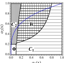
Figure 3: The Acceptance Function with Exponential Signals. The figure depicts the acceptance function ψ(α1) for the case of exponential signals. As their caliber increases,
students apply to nowhere (Φ), college 2 only (C2), both colleges (B) — specifically, first using
college 1 as a stretch school, and later college 2 as a safety school — and finally college 1 only (C1). Student behavior is therefore monotone for the acceptance function depicted.
with 0< αi(x)<1, and the limit behavior limx→0αi(x) = 0 and limx→∞αi(x) = 1.
Taking the acceptance chances as given, each student of caliber xfaces the portfolio optimization problem of §3.1. She must choose a set S(x) of colleges to apply to, and accept the offer of the best school that admits her. We now translate the sets Φ, C2, B, C1
of acceptance chance vectors into corresponding sets of calibers, namely, Φ,C2,B,C1.
Key to our graphical analysis is a quantile-quantile function relating student admis-sion chances at the colleges: Sinceαi(x) strictly rises in the student’s typex, a student’s
admission chance α2 to college 2 is strictly increasing in his admission chance α1 to
college 1. Inverting the admission chance in the type x, the inverse function ξ(α, σ) is the student type accepted with chance α given the admission standard σ, namely
α≡1−G(σ|ξ(α, σ)). This yields an implied differentiable acceptance function
α2 =ψ(α1, σ1, σ2) = 1−G(σ2|ξ(α1, σ1)) (3)
We prove in the appendix that the acceptance function rises in college 1’s standard σ1
and falls in college 2’s standard σ2, and tends to 0 and 1 as thresholds near extremes. By Figure 3, secant lines drawn from the origin or (1,1) to successive points along the acceptance function decrease in slope. To this end, say that a functionh: [0,1]→[0,1] has the double secant property if h(α) is weakly increasing on [0,1] with h(0) = 0,
h(1) = 1, and the two secant slopes h(α)/α and (1−h(α))/(1−α) are monotone inα. This description fully captures how our acceptance chances relate to one another.
Theorem 1 (The Acceptance Function) The acceptance function α2 =ψ(α1) has
the double secant property. Conversely, for any smooth monotone onto function α1(x),
and anyh with the double secant property, there exists a continuous signal densityg(σ|x)
with the strict MLRP, and thresholds σ1, σ2, for which admission chances of student x
to colleges 1 and 2 are α1(x) and h(α1(x)).
This result gives a complete characterization of how student admission chances at two ranked universities should compare. It says that if a student is so good that he is guaranteed to get into college 1, then he is also a sure bet at college 2; likewise, if he is so bad that college 2 surely rejects him, then college 1 follows suit. More subtly, we arrive at the following testable implication about college acceptance chances:
Corollary 1 As a student’s caliber rises, the ratio of his acceptance chances at college 1 to college 2 rises, as does the ratio of his rejection chances at college 2 to college 1.
For an example, suppose that caliber signals have the exponential density g(σ|x) = (1/x)e−σ/x. The acceptance function is then given by the increasing and concave geo-metric function ψ(α1) = α
σ2/σ1
1 , as seen in Figure 3 (as long as college 2 has a lower
admission standard). The acceptance function is closer to the diagonal when signals are noisier, and farther from it with more accurate signals.11 For an extreme case, as
we approach the noiseless case, a student is either acceptable to neither college, both colleges, or just college 2 (assuming that it has a lower admission standard). The ψ
function tends to a function passing through (0,0), (0,1), and (1,1).12
Since a student’s decision problem is unchanged by affine transformations of costs and benefits, we henceforth assume a payoff v = 1 of college 1; so, college 2 pays u ∈(0,1). Throughout the paper,we also realistically assume that application costs are not too high relative to the college payoffs — specifically,c < u(v−u)/v =u(1−u) andc < u/4. The first inequality guarantees that the curves M B21 =cand M B12 =c do not cross twice
inside the unit square.13 The second inequality ensures that the M B
21=ccurve crosses
11Specifically, for the earlier location-scale family,ψ(α
1) rises in the signal accuracy 1/µ(see Persico
(2000)). Easily, the acceptance function tends to the top of the box in Figure 3 as µ → 0, since
ψ(α1) = 1−G(−∞) = 1, and to the diagonalψ(α1) = 1−G(0 +G−1(1−α1)) =α1 asµ→ ∞. 12The limit function is not well-defined: If a student’s type is known, just these three points remain. 13For ifα
2= 1, thenM B21=candM B12=c respectively forceα1= 1−(c/u) andα1=c/(v−u).
below the diagonal.14 If either inequality fails, the analysis trivializes since multiple college applications are impossible for some acceptance functions, as they are too costly.
4
Equilibrium Analysis for Colleges
4.1
A Supply and Demand Approach
Each collegeichooses an admission standardσias a best response to its rival’s threshold
σj and the student portfolios. With a continuum of students, the resulting enrollment
Ei at colleges i= 1,2 is a non-stochastic number (recall thatαi(x)≡1−G(σi|x)):
E1(σ1, σ2) = Z B∪C1 α1(x)f(x)dx (4) E2(σ1, σ2) = Z C2 α2(x)f(x)dx+ Z B α2(x) (1−α1(x))f(x)dx, (5)
suppressing the dependence of the setsB,C1 and C2 on the student application strategy.
To understand (4) and (5), observe that caliber x student is admitted to college 1 with chanceα1(x), to college 2 with chanceα2(x), and finally to college 2 but not college 1 with
chance α2(x)(1−α1(x)). Also, anyone that college 1 admits will enroll automatically,
while college 2 only enrolls those who either did not apply or got rejected from college 1. If we substitute optimal student portfolios into the enrollment equations (4)–(5), then they behave like demand curves where the admissions standards are the prices. Our framework affords analogues to the substitution and income effects in demand theory. The admission rate of any college obviously falls in its anticipated admission standard — the standards effect. But there is a compoundingportfolio effect — that enrollment also falls due to an application portfolio shift. Each college’s applicant pool shrinks in its own admissions threshold. We then deduce in the appendix the “law of demand”: If a college raises its admission standard, then its enrollment falls. Because of our portfolio effect, a college faces a more elastic demand for slots than predicted purely by the standards effect. A lower admission bar will invite applications from new students.15
The law of demand applies outside the two college setting. For intuition, suppose that the admissions standard at a college rises. Absent any student portfolio changes, fewer
14ForM B
21=chas no roots on the diagonalα2=α1ifc > u/4.
15The portfolio effect may act with a lag — for instance, a college may unexpectedly ease admission
students meet its tougher admission threshold (the standards effect), and its enrollment falls. The portfolio adjustment reinforces this effect. Those who had marginally chosen to add this college to their portfolios now excise it (the portfolio effect).
In consumer demand theory, the “price” of one good affects the demand for the other, and in the two good world, they are substitutes. Analogously, we prove in the appendix, that a college’s enrollment demand rises in its rival’s admission standard. This owes to a portfolio spillover effect. If it grows tougher to gain admission to college i, then those who only applied to its rival continue to do so, some who were applying to both now apply just to j (which helps college j when it is the lesser school), and also some at the margin who applied just to i now also add college j to their portfolios.16
Since capacities imply vertical supply curves, we have justified a supply and de-mand analysis, in which the colleges are selling differentiated products. Ignoring for now the possibility that some college might not fill its capacity, equilibrium without excess capacity requires that both markets clear:
κ1 =E1(σ1, σ2) and κ2 =E2(σ1, σ2) (6)
Since each enrollment (demand) function is falling in its own threshold, we may invert these equations. This yields for each school i the threshold that “best responds” to its rival’s admissions threshold σj so as to fill their capacity κi:
σ1 = Σ1(σ2, κ1) and σ2 = Σ2(σ1, κ2) (7)
Given the discussion of the enrollment functions, we can treat Σi as a “best response
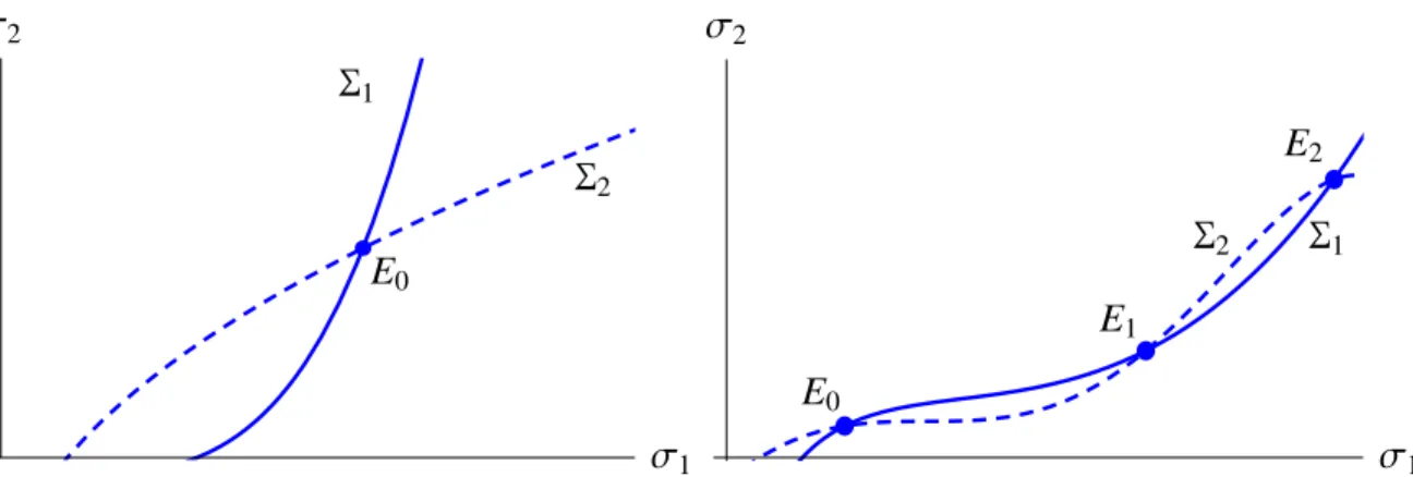
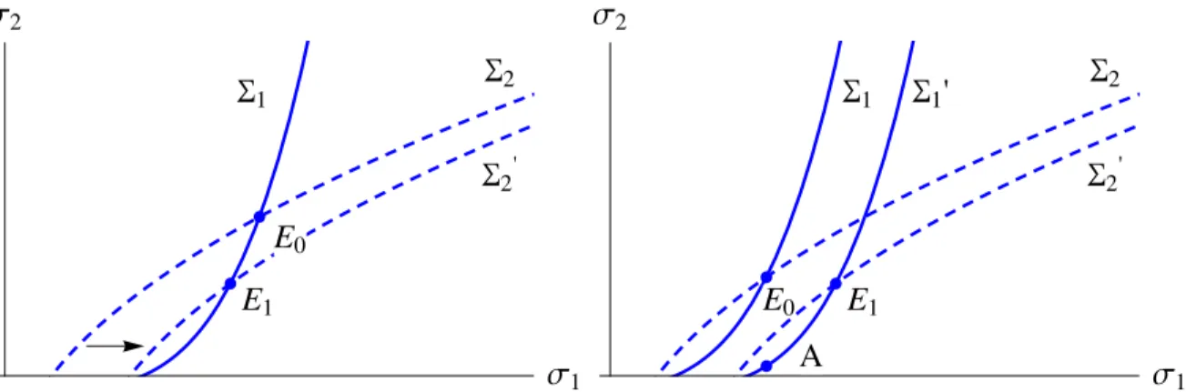
function” of college i. It rises in its rival’s admission standard and falls in its own ca-pacity. That is, the admissions standards at the two colleges are strategic complements. Figure 4 depicts a robust equilibrium as a crossing of these increasing functions.
By way of contrast, observe that without noise or without application costs, the better college is completely insulated from the actions of its lesser rival — Σ1 is vertical.
The equilibrium analysis is straightforward, and there is a unique robust equilibrium. In either case, the applicant pool of college 1 is independent of what college 2 does. For when the application signal is noiseless, just the top students apply to college 1. And
16As in consumer theory, complementarity may emerge with three or more goods available. With
ranked colleges 1, 2, and 3, college 3 may be harmed by tougher admissions at college 1, if this encourages enough applications at college 2.
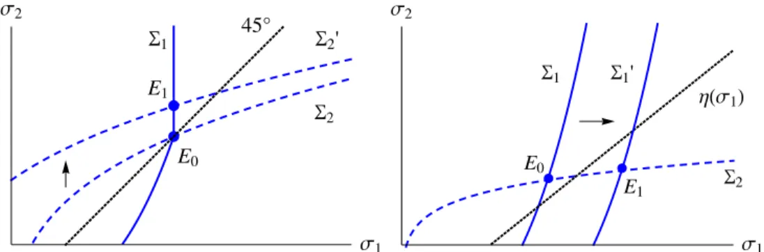
Σ1 Σ2 S1 S2 E0 Σ1 Σ2 S1 S2 E0 E1 E2
Figure 4: College Responses and Equilibria. In both panels, the functions Σ1 (solid)
and Σ2 (dashed) give pairs of thresholds so that colleges 1 and 2 fill their capacities in
equilib-rium. The left panel depicts a unique robust stable equilibrium, while the right panel shows a case with multiple robust equilibria. E0 and E2 are stable, whileE1 is unstable.
when applications are free, all students apply to college 1, and will enroll if accepted. With application costs and noise, Σ1 is upward-sloping, as application pools depend
on both college thresholds. When college 2 adjusts its admission standard, the student incentives to gamble on college 1 are affected. This feedback is critical in our paper. It leads to a richer interaction among the colleges, and perhaps to multiple robust equilibria. In Figure 4, left panel, Σ1 is steeper than Σ2 at the crossing point. Let us call any
such robust equilibriumstable. It is stable in the following sense: Suppose that whenever enrollment falls below capacity, the college eases its admission standards, and vice versa. Then this dynamic adjustment process pushes us back towards the equilibrium. Then at this theoretical level, admission thresholds act as prices in a Walrasian tatonnement. Unstable robust equilibria should be rare: They require that a college’s enrollment responds more to the other school’s admission standard than its own.
Theorem 2 (Existence) A robust stable equilibrium exists. College 1 fills its capacity. Also, there exists κ¯1(κ2, c)<1−κ2 satisfyinglimc→0¯κ1(κ2, c) = 1−κ2 such that if κ1 ≤
¯
κ1(κ2, c), then college 2 also fills its capacity in any robust equilibrium. If κ1 >¯κ1(κ2, c),
then college 2 has excess capacity in some robust equilibrium.
Surprisingly, college 2 may have excess capacity in equilibrium, despite excess demand for college slots.17 This possibility is a consequence of portfolio effects: if college 1 is sufficiently big its standards may be low enough that college 2 fails to attract enough
17College 1 cannot have excess capacity in a robust equilibrium. For then it must set the lowest
applicants to fill its capacity even if it accepts all of them. In this case, α2 = 1 for all
students, and so the acceptance function traverses the top side of the unit square in Figure 3. So as student caliber rises, the lowest students apply to college {2}, higher students to both colleges, and the best students just apply to college{1}. Let us observe in passing that this is a robust sorting equilibrium.
Since admissions standards are strategic complements, multiple robust equilibria are possible (right panel of Figure 4).18 In such a scenario, both colleges raise their standards,
yet students send even more applications, and another robust equilibrium arises.
4.2
Comparative Statics
We now continue to explore the supply and demand metaphor, and derive some basic comparative statics. The potential multiplicity of robust equilibria makes a comparative statics exercise difficult. But fortunately, our analysis applies toall robust stable sorting equilibria and in some cases to all robust stable equilibria. Indeed, at any robust stable equilibrium, greater capacity at either college lowers both college admissions thresholds.
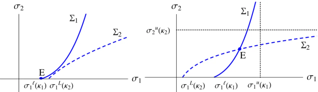
This result speaks to the equilibrium effects at play. Greater capacity at one school, or an exogenous increase in the “supply” of slots at that college, reduces the “price” (admission standard) at both schools. The left panel of Figure 5 proves this assertion for an increase in κ2, and the proof for a change in κ1 is analogous.
For intuition, consider a robust stable sorting equilibrium, where students apply as in Figure 3. Let college 2 raise its capacity κ2. For any admission standard σ1, this
depressesσ2, so Σ2shifts down. Then the marginal student that was indifferent between
applying to college 2 only (C2) and both colleges (B) now prefers to apply to college 2
only. So fewer apply to college 1. Given this portfolio shift, college 1 drops its admission standards, and both thresholds are lower in the new equilibrium E1. The same logic
generates the analogous comparative static for an increase in capacity at college 1. Unlike college capacity, changes in college payoffs or application costs affect both best response functions Σ1 and Σ2. As a result, the comparative statics can be ambiguous,
and counter-intuitive results may emerge. For example, suppose the payoffv of college 1 rises (right panel of Figure 5). At the current admissions standards, demand for college 1 will increase, while demand for college 2 decreases as more of its applicants gamble up on college 1. These forces lead to new best response functions, namely a rightward shift
Σ1 Σ2 S2' S1 S2 E0 E1 Σ1 Σ2 S2' S1 S1' S2 E0 E1 A
Figure 5: Comparative Statics. In both panels, the best response functions Σ1 (solid)
and Σ2 (dashed) are drawn. The left panel considers a rise inκ2, which shifts Σ2 up and has
no effect on Σ1. In the right panel, we illustrate the effect of an increase in college 1’s payoff,
which shifts Σ1 to the right and shifts Σ2 down.
in Σ1 and a downward shift in Σ2.
At first glance, this has ambiguous effects: depending on the size of the shifts, both admissions standards could rise or both could fall, or the standard at college 1 could rise and that of college 2 could fall.19 But provided Σ2 does not fall below the point
A in Figure 5, the new curves Σ01 and Σ02 will cross above and to the right of A. In that case, there is another robust and stable equilibrium in which σ1 rises. Notice that college 2 attracts more applications and admits more students at A than at E0 because
of its lower standards, while losing joint admits at the same rate as before (see the proof of Theorem 3). So it must have excess demand at A, and thus Σ02 must pass between
E0 and A, implying a new equilibrium E1 in which college 1’s standards increase.
Next, assume that the application cost c rises, perhaps due to a rise in the SAT or ACT cost, or the common application fee. This has two effects. On the one hand, it decreases the number of college applications (the region B in Figure 3 shrinks). This has an unambiguously negative effect on demand at both colleges. On the other hand, it decreases competition between the colleges, as there will be fewer overlapping applica-tions. This has no effect on college 1 (since they always beat college 2 for joint admits), but it improves the yield of college 2. As a result, demand at college 1 falls and Σ1 shifts
left, but the effect on Σ2 is ambiguous.
Using an argument similar to the one above, we can show that there exists a new robust stable equilibrium in whichσ1 falls. But due to the competition effect, we cannot
be sure how σ2 moves: college 2 may raise its standards in the new equilibrium, if the higher applications costs deter sufficiently many students from gambling up.
Consider instead a rise in just one college’s application cost, such as a college requiring a longer essay or imposing a greater fee. We argue that in a robust stable sorting equilibrium, if the application cost at either college slightly falls, then the admission standard at college 1 rises and its student caliber distribution stochastically worsens.
For example, if the application cost at college 2 falls, then more students apply, and it is forced to raise its standards. The marginal benefit of a stretch application to college 1 thus rises. To counter this, college 1 responds with a higher standard. Still, its set of applicants is of lower caliber than before (in the sense of the strong set order), and though it screens them more tightly, its caliber distribution stochastically worsens. By contrast, college 2 loses not only its worst students, but also top ones for whom it was insurance, and its caliber change is ambiguous.
Summarizing our results on changes in college payoffs and application costs:
Theorem 3 (Comparative Statics) In a robust stable sorting equilibrium:
(a) When v increases, there exists another robust equilibrium in which σ1 increases.
(b) When c increases, there exists another robust equilibrium in which σ1 decreases.
(c) When either college’s application cost increases marginally, σ1 decreases.
Whenever σ1 decreases due to one of the above changes, the distribution of enrolled calibers at college 1 improves in the sense of first order stochastic dominance.
The final part of the theorem suggests that top-tier colleges have an incentive to increase application costs, since this leads the weakest applicants to self-select out of applying to them. There is some evidence of this: many top-tier colleges require id-iosyncratic essays as part of their application, effectively raising application costs.20 Yet
this result relies on our assumption that students know their type and colleges do not, for if colleges were better than students at identifying caliber, then they might want to encourage applications by lowering application costs. This appears to be true for low-income students: Hoxby and Avery (2012) show that many low-low-income high-achievers act as if they were unaware of their caliber, and do not apply to any selective colleges. In this case top schools should decrease frictions for low-income students, through appli-cation cost waivers and targeted recruiting efforts — both of which we see in practice.
20For example, one essay prompt from the University of Chicago this year is the Winston Churchill
quote that “A joke is a very serious thing”; also, almost all of Amherst’s essay prompts are based on quotes from Amherst professors and alumni.
The logic underlying this section does not essentially depend on the assumption that there are two colleges. For instance, whenever colleges have overlapping applicant pools, a rise in capacity at any one college depresses the admission standards at all of them.
Consider the positive theory of this section in light of Hoxby (2009). She shows that during 1962-2007, the median college has become significantly less selective, while at the same time, admissions have become more competitive at the top 10% of colleges. Her explanation for the fall in standards hinges on capacity: the number of freshman places per high-school graduate has been rising steadily. But as we illustrate in Figure 5, higher capacity at all schools should depress standards at all schools, via our spillover effect. As a countervailing force, she argues that students have simultaneously become more willing to enroll far from home, raising the relative payoff of selective colleges. This aligns with Theorem 3: starting at a robust and stable sorting equilibrium, a perceived increase in the value of an education at a top school leads it to raise its standards.
5
Do Colleges and Students Sort in Equilibrium?
Casual empiricism suggests that the best students apply to the best colleges, and those colleges are in turn the most selective. This logic justifies ranking colleges based on their admissions standards. Curiously, these claims are false without stronger assumptions. We identify and explore two possible types of sorting violations.
The first violation occurs when some relatively high calibers “play it safe”. By Corollary 1, along the acceptance function, higher types enjoy a higher ratio of ad-missions chances at college 1 to college 2. But this does not imply a higher marginal benefit α1(1−α2u) of applying to college 1, and so lower types may apply more
ag-gressively. We illustrate this in the left panel of Figure 6, where application sets are Φ,{2},{1,2},{2},{1,2},{1} as caliber rises. A concrete example is the Texas top 10% plan, which guarantees automatic admission to any school in the UT system for students graduating in the top 10% of their high-school class. Such students have little incentive to apply to slightly better out-of-state schools (college 1), since the payoff increment is small and they don’t need the insurance of a second application. But students who just miss the 10% cutoff may want the insurance, and so one might see more aggressive ap-plication portfolios from those (lower-caliber) students, generating a non-monotonicity. The second violation occurs when the worse college sets a higher admissions stan-dard. To see how this can happen, consider the edge case where the standards are the
0.0 0.2 0.4 0.6 0.8 1.0 0.0 0.2 0.4 0.6 0.8 1.0 Α1HxL Α 2 H x L
C
1F
C
2B
0.0 0.2 0.4 0.6 0.8 1.0 0.0 0.2 0.4 0.6 0.8 1.0 Α1HxL Α 2 H x LC
1F
C
2B
P
Q
Figure 6: Non-Monotone Behavior. In the left panel, the signal structure induces a piecewise linear acceptance function. Student behavior is non-monotone, since there are both low and high caliber students who apply to college 2 only (C2), while intermediate ones insure
by applying to both. In the right panel, equal thresholds at both colleges induce an acceptance function along the diagonal, α1 = α2. Student behavior is non-monotone, as both low and
high caliber students apply to college 1 only (C1), while middling caliber students apply to
both. Such an acceptance function also arises when caliber signals are very noisy.
same at both colleges. With common admissions chances α, the marginal benefit of a safety application (1−α)αu is not increasing in α (and thus not in caliber, either). The right panel of Figure 6 depicts one such case — where the application sets are Φ,{1},{1,2},{1} as caliber rises.In this case college 2 only attracts insurance applica-tions. This can be an equilibrium outcome if college 2 is small enough (and by making it still smaller, college 2 can end up setting a higher standard than college 1).
To rule out the first sorting violation, it suffices that college 2 offer a low payoff
(u <0.5), so that the payoff increment of admission to college 1 is large. We show in the
Appendix that this ensures that the marginal benefit of additionally applying to college is increasing in caliber. The second sort of violation cannot occur when college 1 sets a sufficiently higher admission standard than college 2. This happens when college 1 is sufficiently smaller than college 2. The threshold capacity will depend on the model primitives: rival capacity, applications cost, payoff differential and signal structure.
Theorem 4 (Non-Sorting and Sorting in Equilibrium)
(a)If college 2 is “too good” (i.e.,u >0.5), then there exists a continuous MLRP density
g(σ|x) that yields a robust stable equilibrium with non-monotone student behavior.
standard than college 1 in some robust equilibrium.
(c)If college 1 is small enough relative to college 2, and college 2 is not too good (namely,
u≤0.5), then there are only robust sorting equilibria and no college has excess capacity.
The challenge in proving this theorem is to show that all of non-monotone behavior outlined above can happen in equilibrium. For part (a), we construct a robust non-monotone equilibrium by starting with the acceptance function depicted in the left panel of Figure 6, which constrains the relationships between admissions chances across colleges to be some mapping α2(x) = h(α1(x)). We then construct a particular acceptance
chanceα1(x) so that the induced student behavior and acceptance rates given (α1, h(α1))
equate college capacities and enrollments. Finally, we show that these two mappings satisfy the requirements of Theorem 1 and therefore can be generated by MLRP signals and monotone standards. For part (b), we show that that by perturbing a robust equilibrium with equal admissions chances by making college 2 smaller, we get a robust equilibrium with non-monotone standards. Finally, part (c) turns on showing that when
κ1 is relatively small, the crossing of the best-response functions must occur at a point
where college 1 sets high enough standards that low caliber students don’t apply there. All told, parts (a) and (b) show that sorting may fail, which is surprising given how well behaved the signal structure is. Even in equilibrium, the optimal student portfolio may not increase with caliber; and worse colleges can enroll students of higher average caliber if they are sufficiently small.21 Since organizations like US News and
World Report use statistics like the average SAT score of matriculants in their college rankings, this undercuts how colleges are ranked.
For an insightful counterpoint, consider what happens when students are limited to just a single application, as it is sometimes the case.22 Recalling the left panel in
Figure 2, we see that the diagonal line α1u=α2, and the individual rational equalities
α2u = α1 = c, jointly partition the application space into three relevant parts. But
with any acceptance function with the falling secant property, low types apply nowhere, middle types apply to college 2, and high types apply to college 1. It should come as
21This can be illustrated using the right panel of Figure 6. Consider a robust equilibrium with equal
admissions standards at the two colleges. Iff(x) concentrates most of its mass on the interval of low calibers who apply just to college 1, then the average caliber of students enrolled at college 1 will be strictly smaller than that at college 2. This example can be adjusted slightly so that college 2 is more selective than college 1. (See our online appendix for a fleshed out example of this phenomenon.)
22In Britain, all college applications go through UCAS, a centralized clearing house. A maximum of
no surprise that there is a unique robust equilibrium. So it turns out that the sorting failures in Theorem 4 (a) and (b) require portfolio applications.
Moreover, the college non-monotonicity result requires that colleges have some “mar-ket power”. To see this, suppose that there were instead two tiers of colleges, a top tier 1 and an lesser tier 2; each containing a continuum of otherwise identical colleges with total capacity κ1 and κ2 respectively. Students may apply to multiple colleges within a
tier, each application generating a conditionally iid signal and costing c. Then college standards must be monotone; for if the top tier colleges were easier to get into, no student would ever apply to a second tier college. By contrast, we show in the online appendix that the student non-monotonicity result is robust to making the colleges atomistic.
6
General Incomplete Information About Calibers
A. When Students Do Not Know their Calibers. We have assumed that colleges observe conditionally independent evaluations of the students’ true calibers. At the opposite extreme, one might envision a hypothetical world where colleges know student calibers, and students see noisy conditionally independent signals of them. Yet observe that this is informationally equivalent to a world in which students know their calibers, and colleges observe perfectly correlated signals. For any student sees a signal equal to
t+ “noise”, while both colleges see the student caliber t.
This embedding suggests that we could capture the world in which students and colleges alike only see noisy conditionally iid signals of calibers by relabeling the student signal as their caliber. We argue in the appendix that under this relabeling that world is a special case of the following one:
(F)Students know their calibers and colleges observe affiliated noisy signals of them.
Thus, we can without loss of generality assume that students know their calibers and colleges vary by their signal affiliation.23 Observe that in this world, Theorem 1 remains a valid description of how the unconditional acceptance chances at the two colleges relate.
B. Perfectly Correlated Signals. This benchmark is highly instructive. Suppose first that the two colleges observe perfectly correlated signals of student calibers. As we mentioned above, this is akin to observing the caliber of each applicant. The key (counterfactual) feature here is that if a student is accepted by the more selective college,
then so is he at the less selective one. This immediately implies that σ1 > σ2 in equilibrium, for otherwise no one would apply to college 2. So contrary to Theorem 4,
college behavior must be monotone in any equilibrium.
The analysis of this case differs in a few dimensions from §3.1. Since σ1 > σ2, applying to both colleges now yields payoff α1+ (α2−α1)u−2c. Unlike before,24
M B21≡(α2−α1)u=c and M B12≡α1(1−u) = c (8)
because admission to college 1 guarantees admission to college 2. In this informational world, both optimality equations are linear, and the latter is vertical (see Figure 7).
Assume that college 1 is sufficiently more selective than college 2. Then the lowest caliber applicants apply to college 2 — namely, those whose admission chance exceeds
c/u. Students so good that their admission chance at college 1 is at least c/(1−u) add a stretch application, provided college 2 admits them with chance c/u(1−u) or more. In Figure 7, this occurs when the acceptance function crosses above the intersection point of the curves M B21 = c and M B12 = c.25 Since the marginal benefit M B12 is
independent of the admission chance at college 2, M B12> c for all higher calibers.
But monotone behavior for stronger caliber students requires another assumption. Consider the margin between applying just to college 1, or adding a safety application. The top caliber students will apply to college 1 only, since their admission chance is so high. But the behavior of slightly lesser student calibers is trickier, as the acceptance function can multiply cross the line M B21 =c.26 Under slightly stronger assumptions,
the acceptance function is concave; this precludes such perverse multiple-crossings, and implies monotone student behavior.27
Consider now the possibility of non-monotone student behavior. Absent a concave acceptance function, the previous sorting failure owing to multiple-crossings arises. But even with a concave acceptance function, a sorting failure arises if college 1 is not suffi-ciently choosier than college 2. For then a suitably drawn concave acceptance function could consecutively hit regions C1, B, then C1, and a sorting failure ensues.
Having explored the impact of correlation on college-student sorting, we now flesh
24We suppress the caliberxargument of the unconditional acceptance chanceα
i(x) at collegei= 1,2.
25Namely, at the mutual intersection of regionsC
1, C2, andB in Figure 7. By inequality (13), this
holds under our hypothesis that college 1 is sufficiently choosier than college 2.
26For as seen in Figure 7, that line also has a strictly falling secant. 27Concavity holds whenever−G
x(σ|x) is log-supermodular. This is true when we further restrict to
0.0 0.2 0.4 0.6 0.8 1.0 0.0 0.2 0.4 0.6 0.8 1.0 Α1HxL Α 2 H x L
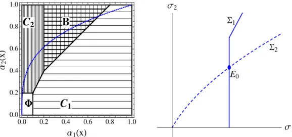
C
1F
C
2B
Σ1 Σ2 S1 S2 E0Figure 7: Student Behavior with Perfectly Correlated Signals. The shaded regions depict the optimal portfolio choices for students when colleges observe perfectly correlated signals. Unlike Figure 2, theM B12=ccurve separating regions B and C2 is vertical. The Σ1
curve at the right is vertical (up to a point), since college 2 no longer imposes an externality on college 1 when the set of calibers sending multiple applications is nonempty.
out its effect on college feedbacks. SinceM B12is independent of the admission threshold
at college 2 in (8), the pool of applicants to college 1 is unaffected by changes in σ2. Hence, the Σ1 locus is vertical over most of its domain.28 The better college is insulated
from the decisions of its weaker rival, and the setting is not as rich as our baseline conditionally iid case. It is obvious from Figure 7 that the robust equilibrium is unique.
C. Affiliated College Evaluations. We now turn to the general case of assumption (F). Each student knows his caliberx, and colleges see signals σ1, σ2 of them, with an
affiliated joint density g(σ1, σ2|x).29 Since acceptance and rejection by college 1 is good
and bad news, respectively, it intuitively follows that
αA2 ≥α2 ≥αR2 (9)
Here, αA
2 and αR2 are the respective acceptance chances at college 2 given acceptance
and rejection at college 1. For instance, 1 = αA
2 > α2 > αR2 with perfectly correlation.
But in the conditionally iid case, college 2 is unaffected by the decision of college 1, and
28The locus Σ
1vertical if college 1 is sufficiently more selective than college 2. For then the acceptance
function is high enough that it traverses regionB, and some students send multiple applications. If not, then the acceptance function could hitC2and thenC1, bipassing regionB. In that case, the marginal
applicant to college 1 depends onσ2, and hence Σ1 is not vertical.
so α2A = α2 = αR2. Since these are intuitively opposite ends of an affiliation spectrum,
we call evaluations more affiliated if the conditional acceptance chance αA
2 at college 2
is higher for any given unconditional acceptance chance α2.
Let’s first see how affiliation affects student applications. In this more general setting,
M B21= (1−α1)αR2u and M B12=α1(1−αA2u). (10)
This subsumes the marginal analysis for our conditionally iid and perfectly correlated cases: (1)–(2) and (8). Relative to these benchmarks, the acceptance curse (or the “acceptance blessing”) conferred by college 1’s two possible decisions lessens the marginal gain of an extra application to either college — due to inequality (9). More intuitively, double admission is more likely when signals are more affiliated. In our graph, this is reflected by a right shift of the curve M B12=c, and a left shift ofM B21 =c. In other
words, for any given college admission standards, students send both fewer stretch and safety applications when college evaluations are more affiliated.
We next explore how affiliated evaluations affects college behavior. Consider the best reply locus Σ1of college 1. It is upward-sloping with conditionally iid college evaluations,
and vertical with perfectly correlated evaluations. We argue that it is upward-sloping with affiliated evaluations, and grows steeper as evaluations grow more affiliated. In other words, our benchmark conditionally iid case delivers robust results about two-way college feedbacks. Perfectly correlated evaluations therefore ignores the effect of the lesser on the better college, and so is less reflective of the affiliated case.
We first show that the best response curve Σ1 slopes upward with imperfect
affilia-tion. For let college 1’s admission standard σ1 rise. Then its unconditional acceptance chance α1 falls for every student. The marginal student pondering a stretch
applica-tion must then fall in order for college 1 to fill its capacity (6). Optimality M B12 = c
in (10) next requires that this student’s conditional acceptance chanceαA
2 fall. This only
happens if his unconditional chance α2 falls too — i.e. the standardσ2 rises.
Next, college 1’s best response curve Σ1 slopes up more steeply when college
eval-uations are more strongly affiliated. For as affiliation rises, the marginal student sees a greater fall in his admission chance αA
2. So his unconditional chance α2 falls more
too, and college 2’s admission standard σ2 drops more than before (see Figure 7), as claimed. As an aside, since robust equilibrium is unique with perfectly correlated college evaluations, uniqueness intuitively holds more often when we are closer to this extreme. Finally, we consider how the equilibrium sorting result Theorem 4 changes with
affili-ation. By examining (10), we see thatas we transition from conditionally iid to perfectly correlated signals with increasing affiliation, the region of multiple applications shrinks monotonically. This simple insight has important implications for sorting behavior. By standard continuity logic, for very low or high affiliation, sorting obtains and fails ex-actly as in the respective conditional independent or perfectly correlated cases. More strongly, the negative result in Theorem 4 (b) fails for moderately high affiliation: For then nonmonotone college behavior is impossible since the locus M B21 = c in (8) lies
strictly above the diagonal, and thus the same holds for (10) with sufficiently affiliated signals. So the acceptance function would lie below the diagonal if admission standards were inverted, and no student would ever apply to college 2. Lastly, the logic for the positive sorting result of Theorem 4 (c) is still valid: both student and college behav-ior are monotone if college 2 is not too small and not too good, and if the acceptance function is concave — appealing to the logic for perfectly correlated signals.
7
The Spillover Effects of Affirmative Action
We now explore the effects of an affirmative action policy.30 Slightly enriching our model, we first assume that a fractionφ of the applicant pool belongs to a target group. This may be an under-represented minority, but it may also be a majority group. For instance, many states favor their own students at state colleges — Wisconsin public colleges can have at most 25% out-of-state students. Just as well, some colleges strongly value athletes or students from low-income backgrounds. We assume a common caliber distribution, so that there is no other reason for differential treatment of the applicants. Assume that students honestly report their “target group” status on their applica-tions. Reflecting the colleges’ desire for a morediverse student body, let collegeiearn a bonus πi ≥0 for each enrolled target student. Colleges may set different thresholds for
the two groups. If collegeioffer a “discount” ∆ito target applicants, then the respective
standards for non-target and target groups are (σ1, σ2) and (σ1−∆1, σ2−∆2). Akin to
third degree price discrimination, now colleges equate the shadow cost of capacity across groups for the marginally admitted student. So at each college, the expected payoff of the marginal admits from the two groups should coincide — except at a corner solution, when a college admits all students from a group. This yields two new equilibrium
condi-30For recent treatment of complementary affirmative action issues, see Epple, Romano, and Sieg
tions that account for the fact that ex post, colleges behave rationally, and equate their expected values of target and non-target applicants. Along with college market clearing (6), equilibrium entails solving four equations in four unknowns.
The analysis is simpler if we assume private values, and we begin with this case. Since colleges care directly about the signal observed with private values, equalization of the marginal admits of the two groups i = 1,2 reduces to σi =σi−∆i+πi, and so
∆i =πi. That is, the ‘discount’ afforded to a student from the target group equals the
additional payoff a college enjoys from admitting a student from the target versus the non-target group. Thus, college preferences for target group students translate directly into admission standard discounts for that group.
Instead, with common values the equalization of shadow values (i.e., the expected payoff of the marginal admits from the two groups) yields the richer conditions:
E[X+π1|σ =σ1−∆1,target] = E[X|σ1,non-target]
E[X+π2|σ=σ2 −∆2,target, accepts] = E[X|σ2,non-target, accepts]
Here, X is the student caliber. As before, along with (6), equilibrium amounts to solving four equations in four unknowns. Notice that no longer do we have ∆i = πi,
which significantly complicates the analysis of the problem. Rather, the discount ∆i
now depends on πi in a nonlinear fashion via the conditional expectations. To obtain a
sharp result, we impose the following notion of stability, which we explain in the online appendix: when the shadow value of a target student exceeds that of a non-target student, college i responds by raising the target advantage ∆i. Call the equilibrium
shadow value stable if this dynamic adjustment process pushes us back to the equilibrium.
Theorem 5 (Affirmative Action) Fix π1 =π2 = 0.
(a) Assume private values and a robust stable equilibrium. As the preference for a target group at one college rises, it favors those students and penalizes non-target students, with no effect on the other college. As the preference π for target students at both colleges rises from π1 =π2 =π = 0, both favor them and penalize non-target ones.
(b) Assume that ∆1 = ∆2 = 0 is a robust shadow value stable equilibrium with
monotone student behavior.31 As the preference for a target group at college 1 rises, it
favors those students and college 2 penalizes them. As the preference for target students at college 2 rises, both colleges favor them more.
Observe the indirect effect of student preferences: Nontarget students face stiffer admis-sion standards since the shadow value of capacity is now higher. The assumption that
π1 = π2 = 0 is important, as it precludes some complex feedback effects that emerge
when there is already a preference for target students at the outset.
Consider private values. For a sharper insight, let the signal distribution beG(σ−x) (location family). Suppose that both colleges exhibit identical preferenceπfor the target group. Since ∆ =πfor both colleges, the acceptance relation isidentical for both groups and given by ψ(α1) = 1−G(σ2 −σ1 +G−1(1−α1)) (the discounts cancel out in the
argument of Gfor the target group). This implies that caliber x from the target group applies exactly as if they were a type x+π from the non-target group: atestable claim. If instead only one college, say 1, has a preference π1 for the target group, then it
sets a discount ∆1 = π1. The acceptance relation for the target group is then ψ(α2) =
1−G(σ2−σ1+ ∆1+G−1(1−α1)), which is everywhere below that of the non-target
groupψ(α2) = 1−G(σ2−σ1+G
−1(1−α
1)). As a result, in a robust sorting equilibrium,
target-group students will gamble up and apply to college 1 more often, and insure with an application to college 2 less often, than non-target group students.
Regarding common values, Theorem 5 (b) (proof in the online appendix) asserts that as the preference for