Forecasting foreign exchange rates with adaptive neural networks using radial basis functions and particle swarm optimization

(1)

Sermpinis, G., Theofilatos, K., Karathanasopoulos, A., and Dunis, C.

(2013) Forecasting foreign exchange rates with adaptive neural networks

using radial basis functions and particle swarm optimization. European

Journal of Operational Research, 225 (3). pp. 528-540. ISSN 0377-2217

A copy can be downloaded for personal non-commercial research or

study, without prior permission or charge

The content must not be changed in any way or reproduced in any format

or medium without the formal permission of the copyright holder(s)

http://eprints.gla.ac.uk/71870/

(2)

Accepted Manuscript

Innovative Applications of O.R

Forecasting foreign exchange rates with adaptive neural networks using radial-basis functions and particle swarm optimization

Georgios Sermpinis, Konstantinos Theofilatos, Andreas Karathanasopoulos, Efstratios F. Georgopoulos, Christian Dunis

PII: S0377-2217(12)00766-7

DOI: http://dx.doi.org/10.1016/j.ejor.2012.10.020

Reference: EOR 11325

To appear in: European Journal of Operational Research Received Date: 30 June 2012

Accepted Date: 19 October 2012

Please cite this article as: Sermpinis, G., Theofilatos, K., Karathanasopoulos, A., Georgopoulos, E.F., Dunis, C., Forecasting foreign exchange rates with adaptive neural networks using radial-basis functions and particle swarm optimization, European Journal of Operational Research (2012), doi: http://dx.doi.org/10.1016/j.ejor.2012.10.020

This is a PDF file of an unedited manuscript that has been accepted for publication. As a service to our customers we are providing this early version of the manuscript. The manuscript will undergo copyediting, typesetting, and review of the resulting proof before it is published in its final form. Please note that during the production process errors may be discovered which could affect the content, and all legal disclaimers that apply to the journal pertain.

(3)

Forecasting foreign exchange rates with adaptive neural networks

using radial-basis functions and particle swarm optimization

by Georgios Sermpinis* Konstantinos Theofilatos** Andreas Karathanasopoulos*** Efstratios F. Georgopoulos**** Christian Dunis ***** October 2012 Abstract

The motivation for this paper is to introduce a hybrid Neural Network architecture of Particle Swarm Optimization and Adaptive Radial Basis Function (ARBF-PSO), a time varying leverage trading strategy based on Glosten, Jagannathan and Runkle (GJR) volatility forecasts and a Neural Network fitness function for financial forecasting purposes. This is done by benchmarking the ARBF-PSO results with those of three different Neural Networks architectures, a Nearest Neighbors algorithm (k-NN), an autoregressive moving average model (ARMA), a moving average convergence/divergence model (MACD) plus a naïve strategy. More specifically, the trading and statistical performance of all models is investigated in a forecast simulation of the EUR/USD, EUR/GBP and EUR/JPY ECB exchange rate fixing time series over the period January 1999 to March 2011 using the last two years for out-of-sample testing.

As it turns out, the ARBF-PSO architecture outperforms all other models in terms of statistical accuracy and trading efficiency for the three exchange rates.

Keywords

Adaptive Radial Basis Function, Partial Swarm Optimization, Forecasting, Quantitative Trading Strategies

_______

*

Georgios Sermpinis University of Glasgow Business School, University of Glasgow, Adam Smith Building, Glasgow, G12 8QQ, UK (E-mail: [email protected])

**Konstantinos Theofilatos Department of Computer Engineering & Informatics, University of Patras, 26500, Patras, Greece (E-mail: [email protected])

***Andreas Karathanasopoulos London Metropolitan Business School,London Metropolitan University, 31 Jewry Street, London, EC3N 2EY, UK (E-mail: [email protected])

**** Efstratios Georgopoulos, Technological Educational Institute of Kalamata, 24100, Kalamata, Greece, (Email: [email protected])

*****Christian Dunis Horus Partners Wealth Management Group SA, Genève, Suisse and Liverpool Business School, JMU, John Foster Building, Liverpool L3 5UZ (E-mail: [email protected])

(4)

1. INTRODUCTION

Neural networks (NN) are an emergent technology with an increasing number of real-world applications including operational research (Lisboa and Vellido (2000) and Zhang et. al. (1998)). However their numerous limitations and contradictory empirical evidence around their forecasting power are often creating scepticism about their use among practitioners. This scepticism is further fuelled by the fact that the selection of each algorithm parameters and inputs is based more on trial and error and the practitioner’s market knowledge rather than on some formal statistical procedure.

The motivation for this paper is to introduce in Operational Research a hybrid Neural Network architecture of Particle Swarm Optimization and Adaptive Radial Basis Function (ARBF-PSO), which try to overcome some of these limitations. More specifically our proposed architecture is fully adaptive something that decreases the numbers of parameters that the practitioner needs to experiment while on the other hand it increases the forecasting ability of the network. The proposed methodology is superior in comparison to the application of meta-heuristic methods (PSO, Genetic Algorithms, Swarm Fish Algorithm) that have been already presented in the literature (Nekoukar and Beheshti (2010) and Shen et al. (2011)) because it eradicates the risk of getting trapped into local optima and the final solution is assured to be optimal for a subset of the training set.

In our study we benchmark our proposed algorithm with a Multi-Layer Perceptron (MLP), a Recurrent Neural Network (RNN), a Psi Sigma Neural Network (PSI), a Nearest Neighbors algorithm (k-NN), an autoregressive moving average model (ARMA), a moving average convergence/divergence model (MACD) plus a naïve strategy in a forecasting and trading simulation of the EUR/USD, the EUR/GBP and the EUR/JPY European Central Bank (ECB) daily fixing. The main reason behind our decision to use the ECB daily fixings is that it is possible to leave orders with a bank and trade on that basis. It is therefore a tradable quantity which makes our trading simulation more realistic. We examine the exchange rates from their first trading day since the end of April 2011. Moreover, the nonlinearities and the high complexity of the exchange rates series make them perfect for a forecasting exercise. Nevertheless our proposed methodology can be applied to any forecasting task irrespective the nature of the series under study.

Moreover, we introduce a time-varying leverage trading strategy based on GJR (1993) model volatility forecasts and examine if its application can increase the trading efficiency of our models.

(5)

We also introduce a fitness function for our NNs that not only minimize the MSE of our forecasts but also increase their profitability. This is crucial in financial applications where statistical accuracy is not always synonymous with financial profitability of the derived forecasts.

As it turns out the ARBF-PSO algorithm does remarkably well and outperforms all other models in terms of statistical accuracy and trading efficiency for the time series and period under study. It seems that its adaptability and flexibility allows it to outperform in our forecasting competition compared with the more ‘traditional’ k-NN, MLP, RNN and PSI models. These results provide the first empirical evidence around the utility of the ARBF-PSO in finance and forecasting.

The rest of the paper is organised as follows. In section 2 we present some relevant recent applications in forecasting and section 3 describes the dataset used for this research and its characteristics. An overview of the proposed model and the NN and statistical benchmarks is given in section 4. Section 5 gives the empirical results of all the models considered and investigates the possibility of improving their performance with the introduction of a sophisticated trading strategy while section 6 provides some concluding remarks.

2. LITERATURE REVIEW

Developing high accuracy techniques for predicting time series is a very crucial problem for scientists and decision makers. The traditional statistical methods seem to fail to capture the discontinuities, the nonlinearities and the high complexity of datasets such as financial time series. Complex machine learning techniques like Artificial Neural Networks (NNs) provide enough learning capacity and are more likely to capture the complex non-linear models which are dominant in the financial markets but their parameter tuning remains difficult and generalization problems exist (Donaldson and Kamstra (1996) and Lisboa and Vellido (2000)). The main objective of this paper is to introduce a novel hybrid method which is able to overcome the difficulties in tuning the parameters of artificial neural networks. For this purpose among the various neural network techniques, we use the Radial Basis Function Neural Networks (RBFNN) which has proven experimentally to outperform the more classical NNs architectures (Broomhead and Lowe (1988)). The hybrid method combines the RBFNNs with Particle Swarm Optimization (PSO) algorithm, a state-of-the art heuristic optimization technique (Kennedy and Eberhart (1995)) in a way that optimizes the neural networks parameters,

(6)

structure and training procedure. Our proposed methodology is an extension of the algorithm proposed by Ding et. al. (2005) for forecasting purposes.

The proposed methodology has not been applied in science yet. However, two approaches have been recently proposed for the optimization of RBF Neural Networks and their application in financial time-series forecasting. Nekoukar and Beheshti (2010) propose the application of a modified PSO (using hunter particles to increase diversity) for training Radial Basis Functions. This methodology was applied for the prediction of the price of Iranian stock time-series. Despite the high prediction accuracy of the derived model, this hybrid technique does not provide any method for optimizing the structure of the RBF network. Moreover, the applied PSO algorithm uses constant parameters, which requires an extra time-consuming optimization step. Shen et al. (2011) introduce a novel hybrid technique which applies an Artificial Fish Swarm algorithm to train Radial Basis Function Neural Networks for modeling the Shanghai Composite Indices. The prediction results are extremely good, but the artificial fish swarm algorithm is not used for the optimization of the RBF network’s structure and it requires some parameters to be tuned via a time consuming trial and error approach. Compared to a simple genetic algorithm and a simple PSO method which are also used to train Radial Basis Function Neural Networks, the Artificial Fish Swarm algorithm produces a slightly higher prediction error but the authors believe that being a new intelligent algorithm it has room for improvement and development. Both of these methods use Mean Square Error as a fitness function and they are not specialized for the prediction of financial time series contrary to our proposed methodology.

Several scientists have applied other NNs algorithms to the task of forecasting financial series with ambiguous empirical evidence. Fulcher et. al. (2006) apply Higher Order Neural Networks in forecasting the AUD/USD exchange rate with a 90% accuracy. Panda and Narasimhan (2007) use a single hidden layer feedforward NN to produce statistical accurate forecasts of the INR/USD exchange rate having several linear autoregressive models as benchmarks while Andreou et. al. (2008) use NNs to forecast and trade European options with disappointing results. On the other hand, Kiani and Kastens (2008) forecast the GBP/USD, the CAD/USD and the JPY/USD exchange rates with feedforward and recurrent NNs having as benchmarks several ARMA models. In their application, NNs outperform in statistical terms their ARMA benchmarks in forecasting the GBP/USD and USD/JPY but not in forecasting the USD/CAD exchange rate. Yang et. al. (2008) employ a NN and other regression techniques to examine the potential martingale behaviour of Euro exchange rates in the context of out-of-sample forecasts. The overall evidence indicates that, while martingale behaviour cannot be rejected for Euro

(7)

exchange rates with major currencies such as the Japanese yen, British pound, and US dollar, there is nonlinear predictability in terms of economic criteria with respect to several smaller currencies (such as the Australian dollar, the Canadian dollar and the Swiss franc). Bekiros and Georgoutsos (2008) forecast and trade successfully the NASDAQ index with RNNs and Yang et. al. (2010) study the predictability of eighteen stock indexes with NNs and linear models. Their models demonstrate low predictability when the data snooping bias was considered. On the same year while on the same year Huck (2010) combines NNs with a multi-criteria decision making method in a S&P 100 stock pair trading application with good results. Adeodato et. al. (2011) won the NN3 Forecasting Competition problem with an innovative approach based on the use of median for combining MLP forecasts and Matias and Reboredo (2012) forecast successfully with NNs and other nonlinear models intraday stock market returns. In a forecasting competition, Dunis et. al. (2010 and 2011) and Sermpinis et. al. (2012) compare several Higher Order NNs and autoregressive models in forecasting and trading the EUR exchange rates. Their results demonstrate the forecasting superiority of a class of NNs, the Psi Sigma, which are able to capture higher order correlation within their dataset. Bekiros (2010) introduced a promising hybrid neurofuzzy system which forecast accurately the direction of the market for 10 of the most prominent stock indices of U.S.A, Europe and Southeast Asia and Dhamija and Bhalla (2011) apply several variants of the MLP and RBF networks to the task of forecasting five different exchange rates with good results. On the same year Wang et. al. (2011) forecast successfully the Shenzhen Integrated Index and the Dow Jones Industrial Average Index with a hybrid NN model. Compared to the above mentioned studies, our proposed algorithm is fully adaptive and enables us to avoid the time consuming and risky process of optimizing the parameters of our networks through a sensitivity analysis in the in-sample period. However, we apply some of the most promising architectures of the previous mentioned paper such as the Psi Sigma (Fulcher et. al. (2006), Dunis et. al. (2010 and 2011) and Sermpinis et. al. (2012)), the RNN (Kiani and Kastens (2008) and Bekiros and Georgoutsos (2008)) and the MLP (Panda and Narasimhan (2007), Adeodato et. al. (2011) and Dhamija and Bhalla (2011)) as benchmarks to our proposed model.

3. THE EUR/USD AND EUR/GBP EXCHANGE RATES AND RELATED FINANCIAL DATA

The European Central Bank (ECB) publishes a daily fixing for selected EUR exchange rates: these reference mid-rates are based on a daily concentration procedure between central banks within and outside the European System of Central Banks, which normally takes place at 2.15 p.m. ECB time. The reference exchange rates are published both by electronic market

(8)

information providers and on the ECB's website shortly after the concentration procedure has been completed. Although only a reference rate, many financial institutions are ready to trade at the EUR fixing and it is therefore possible to leave orders with a bank for business to be transacted at this level.

The ECB daily fixings of the EUR exchange rates are therefore tradable levels which makes using them a more realistic alternative to, say, London closing prices and these are the series that we investigate in this paper. We examine the ECB daily fixings of the EUR/USD, the EUR/GBP and the EUR/JPY since their first trading day on 4 January 1999 until 29 April 2011. The data period is partitioned as table 1.

Name of period Beginning End

Total dataset 3158 4 January 1999 29 April 2011

Training dataset 2645 4 January 1999 30 April 2009

Out-of-sample dataset [Validation set] 513 4 May 2009 29 April 2011

Table 1: The total dataset

The figure 1 below shows the total dataset for the three exchange rates under study.

Fig. 1: EUR Frankfurt daily fixing prices (total dataset)

The three observed time series are non-normal (the Jarque-Bera statistics confirms this at the 99% confidence level) containing slight skewness and high kurtosis. They are also nonstationary and hence we decided to transform them into a stationary daily series of rates of return1 using the formula:

⎟⎟⎠ ⎞ ⎜⎜⎝ ⎛ = −1 ln t t t P P R [1]

(9)

The summary statistics of the EUR/USD, EUR/GBP and EUR/JPY returns series reveal positive skewness and high kurtosis. The Jarque-Bera statistic confirms again that the two return series are non-normal at the 99% confidence level. These two return series will be forecasted from our models.

In the absence of any formal theory behind the selection of the inputs of a neural network, we conduct neural networks experiments and a sensitivity analysis on a pool of potential inputs in the training dataset in order to help our decision. Based on these experiments and the sensitivity analysis we select as inputs the sets of variables that provide the higher trading performance for each network in the in-sample period. This set of inputs (which is different for each network and series under study) is consisted by a set of autoregressive terms of the three exchange rates under study. We also explored autoregressive terms of other exchange rates as inputs (e.g. the ECB fixing of the EUR/CHF), commodities prices (e.g. Gold Bullion and Brent Oil) and stock market prices (e.g. the S&P 500 index). However, they did not seem to add any value during our sensitivity analysis.2

In order to train our neural networks we further divide our dataset as in table 2:

Name of period Trading days Beginning End

Total dataset 3158 4 January 1999 29 April 2011

Training data set 2134 4 January 1999 30 April 2007

Test data set 511 2 May 2007 30 April 2009

Out-of-sample data set [Validation set] 513 4 May 2009 29 April 2011

Table 2: The neural networks datasets

4. FORECASTING MODELS

4.1 Statistical/Technical Models

In this paper, we benchmark our ARBF-PSO model with 3 different NNs, a Nearest Neighbors algorithm (k-NN) algorithm and 3 traditional strategies, namely an autoregressive moving average model (ARMA), a moving average convergence/divergence technical model (MACD) and a naïve strategy. The performance of our models is evaluated in terms of statistical accuracy and trading performance via a simulated trading strategy.

4.1.1 Naïve strategy

1_{Confirmation of its stationary property is obtained at the 1% significance level by both the Augmented Dickey}

Fuller (ADF) and Phillips-Perron (PP) test statistics.

2_{The 12 different sets of inputs for our 4 different NN architectures and 3 series under study are not presented here}

(10)

The naïve strategy simply takes the most recent period change as the best prediction of the future change. The model is defined by3:

t

t Y

Yˆ+1 = [2]

where Y_t is the actual rate of return at period t

Yˆ_t₊₁ is the forecast rate of return for the next period

4.1.2 Moving Average

A moving average model is defined as:

(

)

n Y Y Y Y M t t t t n t 1 2 1 ... ₋ ₊ − − + + + + = [3]

where Mt is the moving average at time t

n is the number of terms in the moving average

t

Y is the actual rate of return at period t

The MACD strategy used is quite simple. Two moving average series are created with different moving average lengths. The decision rule for taking positions in the market is straightforward. Positions are taken if the moving averages intersect. If the short-term moving average intersects the term moving average from below a ‘long’ position is taken. Conversely, if the long-term moving average is intersected from above a ‘short’ position is taken4.

The forecaster must use judgement when determining the number of periods on which to base the short-term and long term moving averages. The combinations that performed best over the in-sample sub-period were retained for out-of-sample evaluation. The models selected were a combination of (1,8) for the EUR/USD, (3,6) for the EUR/GBP and (2,5) for the EUR/JPY exchange rate.

4.1.3 ARMA model

Autoregressive moving average models (ARMA) assume that the value of a time series depends on its previous values (the autoregressive component) and on previous residual values (the moving average component)5.

The ARMA model takes the form:

q t q t t t p t p t t t Y Y Y w w w Y =φ₀+φ₁ ₋₁+φ₂ ₋₂+...+φ ₋ +ε − ₁ε ₋₁− ₂ε₋₂−...− ε ₋ _[4]

where Yt is the dependent variable at time t

3_{We also applied a simple random walk model to our series (}

t t

Yˆ+1=λ+ε where εt ~N(0,1)and λ is the

in-sample mean). The performance of the random walk model was similar or slightly worse from our naïve strategy as it is described in equation [2] in the in-sample period and is available upon request.

4_{For example, a ‘long’ EUR/USD position means buying Euros at the current price, while a ‘short’ position means}

selling Euros at the current price.

(11)

1 −

t

Y , Yt−2, and Yt−p are the lagged dependent variable 0

φ , φ1, φ2, and φp are regression coefficients t

ε is the residual term 1

−

t

ε , εt−2, and εt−p are previous values of the residual 1

w , w2, and wq are weights.

Using as a guide the correlogram and the information criteria in the training and the test sub periods we have chosen a restricted ARMA (5,5) for the EUR/USD and a restricted ARMA (6,6) for the EUR/GBP and a restricted ARMA (4,4) for the EUR/JPY exchange rate. In all models all their coefficients are significant at the 95% confidence interval as the null hypothesis that all coefficients (except the constant) are not significantly different from zero is rejected at the 95% confidence interval.

The selected ARMA models for the EUR/USD, EUR/GBP and EUR/JPY exchange rates are presented in equations [5], [6] and [7] respectively:

5 3 2 1 5 3 2 1 43699 . 0 285219 . 0 49545 . 0 48310 . 0 40105 . 0 31984 . 0 53617 . 0 49349 . 0 00071 . 0 − − − − − − − − + − + − − + − + = t t t t t t t t t Y Y Y Y Y ε ε ε ε [5] 6 2 1 6 2 1 49460 . 0 44556 . 0 46933 . 0 53005 . 0 43358 . 0 42524 . 0 00011 . 0 − − − − − − − + + + − − = t t t t t t t Y Y Y Y ε ε ε [6] 4 3 1 4 3 1 60691 . 0 056206 . 1 89816 . 0 57035 . 0 02907 . 1 87062 . 0 00036 . 0 − − − − − − − − + + + − = t t t t t t t Y Y Y Y ε ε ε [7] The model selected was retained for out-of-sample estimation.

4.1.4 Nearest Neighbours Model

Nearest Neighbours is a nonlinear and non-parametric forecasting method. It is based on the idea that pieces of time series in the past have patterns which might have resemblance to pieces in the future. Similar patterns of behaviour are located in terms of nearest neighbours using a distance called the Euclidean distance and these patterns are used to predict behaviour in the immediate future. It only uses local information to forecast and makes no attempt to fit a model to the whole time series at once. It is similar to technical analysis as it tries to find out patterns based on certain parameters. The user defines parameters such as the number of neighbours K, the length of the nearest neighbour’s pattern m (also called the ‘embedding dimension’) and the weighting of final prices in a neighbour α. When α is greater than 1, a greater emphasis is given to similarity between the more recent observations. The nearest neighbours algorithm weights the nearest to furthest Neighbour sets according to the Euclidean distance from the actual time

(12)

series. These three parameters are very important for neighbours and very easy to apply computationally.

Guégan and Huck (2004) suggest that a good approximation for choosing the parameters K and m is dependent on the size of the information set. They choose m from the interval:

m = [R(ln(T)), R(ln(T)+2)] [8] where R is the rounding function rounding to the immediate lower figure and T the size of the dataset. They also suggested that K should be approximately twice the value of m. Thus for our dataset m lies between 8 and 10 and K lies between 16 and 20. Based on the above guidelines and Dunis and Nathani (2007) who applied Nearest Neighbours in financial series, we experiment in the in-sample dataset and we select the set of parameters that provide the highest trading performance in the in-sample period. These sets of parameters for each exchange rate under study are presented in table 3 below.

Table 3: Nearest Neighbours Parameters

4.2 Neural Networks

4.2.1. Benchmark Neural Networks Architectures

Neural networks exist in several forms in the literature. The most popular architecture is the Multi-Layer Perceptron (MLP). A standard MLP has at least three layers. The first layer is called the input layer (the number of its nodes corresponds to the number of explanatory variables). The last layer is called the output layer (the number of its nodes corresponds to the number of response variables). An intermediary layer of nodes, the hidden layer, separates the input from the output layer. Its number of nodes defines the amount of complexity the model is capable of fitting. In addition, the input and hidden layer contain an extra node called the bias node. This node has a fixed value of one and has the same function as the intercept in traditional regression models. Normally, each node of one layer has connections to all the other nodes of the next layer.

The training of the network (which is the adjustment of its weights in the way that the network maps the input value of the training data to the corresponding output value) starts with randomly

m K a

EUR/USD 8 18 1.1 EUR/GBP 8 19 1

(13)

chosen weights and proceeds by applying a learning algorithm called backpropagation of errors6 (Shapiro (2000)).The iteration length is optimised by maximising a fitness function in the test dataset.

In addition to the classical MLP network, we also apply a recurrent neural network. While a complete explanation of RNN models is beyond the scope of this paper, we present below a brief explanation of the RNN architecture. For an exact specification of recurrent networks, see Elman (1990). A simple recurrent network has an activation feedback which embodies short-term memory. In other words, the RNN architecture can provide more accurate outputs because the inputs are (potentially) taken from all previous values. The advantages of using recurrent networks over feedfoward networks (such as the MLPs) for modelling non-linear time series, has been well documented in the past (see amongst other Elman (1990) and Tenti (1996)). However as mentioned by Tenti (1996), “the main disadvantage of RNNs is that they require substantially more connections, and more memory in simulation than standard backpropagation networks” (p.569), thus resulting in a substantial increase in computational time. However, having said this, RNNs can yield better results in comparison with simple MLPs due to the additional memory inputs.

The third NN benchmark model considered in our study is the Psi Sigma. Psi Sigma networks can be considered as a class of feedfoward fully connected higher order neural networks. First introduced by Shin and Ghosh (1991), the Psi Sigma network utilizes product cells as the output units to indirectly incorporate the capabilities of higher-order networks while using a fewer number of weights and processing units. Their creation was motivated by the need to create a network combining the fast learning property of single layer networks with the powerful mapping capability of higher order neural networks while avoiding the combinatorial increase in the required number of weights. The order of the network in the context of Psi Sigma is represented by the number of hidden nodes. In a Psi Sigma network the weights from the hidden to the output layer are fixed to 1 and only the weights from the input to the hidden layer are adjusted, something that greatly reduces the training time. Moreover, the activation function of the nodes in the hidden layer is the summing function while the activation function of the output layer is a sigmoid. More details on the Psi Sigma architecture can be found in Shin and Ghosh (1991), Dunis et. al. (2010 and 2011) and Sermpinis et. al. (2012).

4.2.2. Proposed Fitness Function and NN optimization

6

Backpropagation networks are the most common multi-layer networks and are the most commonly used type in financial time series forecasting (Kaastra and Boyd (1996)).

(14)

In our networks which are specially designed for financial purposes we apply a novel multi-objective fitness function. This fitness function focuses on achieving three goals at the same time. First of all, the annualized return in the training period should be maximized and secondly the Mean Square Error (MSE) of the networks output should be minimized. Finally, we are interested in finding the simplest neural network that achieves these goals and thus the number of hidden neuron should be minimized. Based on the above the fitness function for all our networks takes the form of the equation below7:

Fitness= Annualized_Return – MSE – 10-2 _*_{number_of_hidden_neurons [9]} To the best of our knowledge no similar approach has been applied yet in the relevant literature

and equation [9] is an original contribution of this paper. The existing financial forecasting approaches guide their predictors using as fitness functions statistical measures such as the MSE (e.g. Fulcher et. al. (2006)), the RMSE (e.g. Panda and Narasimhan (2007)) or the correct directional movement prediction rate (e.g. Dunis et. al. (2010 and 2011)). However, statistical accuracy does not always imply financial profitability. The proposed fitness function aims to bring a balance between trading profitability (first factor of equation [9]) and statistical accuracy (second factor). Thus, the proposed fitness function clearly outperforms existing fitness functions as our main goal is to extract a profitable trading strategy and not only a prediction that presents low error measures.

After our networks are optimized, the predictive value of each model is evaluated by applying it to the validation dataset (out-of-sample dataset). Since the starting point for each network is a set of random weights, forecasts can differ between networks. In order to eliminate any variance between our NN forecasts, we use the average of a committee of 10 NNs which present the highest profit in the test sub-period. In our study we apply our NNs to the task of forecasting the daily return of the EUR/USD, EUR/GBP and EUR/JPY exchange rates. The characteristics of the NNs used in this paper are presented in Appendix A.1.

4.2.3 ARBF-PSO method

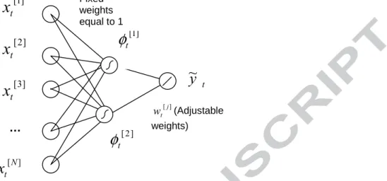
4.2.3.1 Radial Basis Function Neural Networks (RBFNN)

A radial basis function neural network (RBFNN) is a feedforward neural network where hidden units do not implement an activation function, but a radial basis function. An RBFNN approximates a desired function by superposition of nonorthogonal, radially symmetric functions. They have been proposed by Broomhead and Lowe (1988) as an approach to improve

7_{The number of hidden neurons is multiplied with 10}-2_{because the simplicity of the derived neural network is of}

(15)

accuracy of artificial neural networks while decreasing training time complexity. Their architecture is depicted in Figure 2.

Fig. 2: A RBF Neural Network with N inputs and 2 hidden nodes

t

x

(

n=1,2,h ,N+1

)

are the model inputs (including the input bias node)

t y ~ is the RBFNN output ] [j t

w

(j=1,2) are the adjustable weights is the Gaussian function: 2

2 2 ] [

(

)

_i i t C x t i

x

e

σ

φ

− −

=

[10]

where Ci is a vector indicating the centre of the Gaussian Function and σi is a value indicating its width. Ci, σi and the weights wi are parameters which should be optimized through a learning phase in order to train the RBFNN.

is the linear output function:

( )

=

∑

i

F _φ _φ[]_[11] The error function to be minimised is:

(

)

∑

(

)

= − = T t t t t t y y w C T w C E 1 2 , , ~ 1 , ,σ σ [12] with yt being the target value and T the number of iterations.

4.2.3.2 ARBF-PSO method

The hybrid methodology proposed in the present paper is an extension of the hybrid algorithm proposed by Ding et. al. (2005). In this algorithm the Particle Swarm Optimization (PSO) methodology was used to locate the parameters Ci of the RBFNN while in parallel locating the optimal number for the hidden layers of the network. This methodology is extended in our proposed algorithm in order to increase accuracy, make it appropriate for predicting financial time series and avoid the time consuming step of optimizing the parameters of PSO.

MSE). t

y

~

] 2 [ t

φ

] 1 [ t

φ

] 1 [ t

x

] 2 [ t

x

] 3 [ t

x

… ] [N t

x

Fixed weights equal to 1 ] [j t w (Adjustable weights)

(16)

The PSO algorithm, proposed by Kennedy and Eberhart (1995), is a population based heuristic search algorithm based on the simulation of the social behavior of birds within a flock. In PSO, individuals which are referred to as particles are placed initially randomly within the hyper dimensional search space. Changes to the position of particles within the search space are based on the social-psychological tendency of individuals to emulate the success of other individuals. The consequence of modeling this social behavior is that the search process is such that particles stochastically return towards previously successful regions in the search space.

The performance of an RBFNN highly depends on its structure and on the effective calculation of the RBF function’s centers Ci and widths σ and the network’s weights. If the centers of the RBF are properly estimated then their widths and the networks weights can be computed accurately with existing heuristic and analytical methodologies which described below in this paper. In this approach the PSO searches only for optimal values of the parameters Ci and for the optimal number of hidden neurons (the RBFNN structure) which should be used. Each particle i is initialized randomly to have mi hidden neurons (within a predefined interval starting from the number of inputs until 100 which is the maximum hidden layer size that we applied) and is represented as shown in equation [13]:

⎥ ⎥ ⎥ ⎥ ⎥ ⎥ ⎥ ⎥ ⎥ ⎥ ⎥ ⎥ ⎥ ⎥ ⎥ ⎦ ⎤ ⎢ ⎢ ⎢ ⎢ ⎢ ⎢ ⎢ ⎢ ⎢ ⎢ ⎢ ⎢ ⎢ ⎢ ⎢ ⎣ ⎡ = N N N N N N N N c c c c c c c c c C i d m i m i m i d i i i d i i i i i i . ... . . . ... . . . ... . . ... . ... . . . ... . . . ... . . ... ... 2 1 2 22 21 1 12 11 [13]

where N is a large number to point that it does not represent an RBF centre. Using this specific representation scheme, we allow the production of RBFNNs with fewer hidden nodes than the maximum allowed hidden layers size. Thus, the produced optimization algorithm becomes even more flexible and enables the algorithm to locate the optimal network structure for each problem. By optimizing equation [13] the identification of the RBFNN structure and the effective calculation of the RBF function centers can be accomplished in parallel.

In our PSO variation, initially we create a random population of particles, with candidate solutions represented as showed in equation [13], each one having an initially random velocity

(17)

matrix to move within the search space. It is this velocity matrix that drives the optimization process, and reflects both the experiential knowledge of the particle and socially exchanged information from the particles neighborhood. The form of the velocity matrix for every particle is described in the equation below:

⎥ ⎥ ⎥ ⎥ ⎥ ⎥ ⎥ ⎥ ⎥ ⎥ ⎥ ⎥ ⎥ ⎥ ⎥ ⎦ ⎤ ⎢ ⎢ ⎢ ⎢ ⎢ ⎢ ⎢ ⎢ ⎢ ⎢ ⎢ ⎢ ⎢ ⎢ ⎢ ⎣ ⎡ = N N N N N N v v v v v v v v v V i d m i m i m i d i i i d i i i i i i ... . ... . . . ... . . . ... . . ... ... . ... . . . ... . . . ... . . ... ... 2 1 2 22 21 1 12 11 [14]

From the centers of its particle described in equation [13] using the Moody-Darken (1989) approach we compute the RBF widths using the following equation:

i k i j i j = c −c σ [15] where i k

c is the nearest neighbor of the centers i j

c . For the estimation of the nearest neighbors we apply the Euclidean distance which is computed for every pair of centers.

At this point of the algorithm the centers and the widths of the RBFNN have been computed. The computation of its optimal weights wi is accomplished by solving the equation:

Y H H H w T i i T i i ₌₍ _⋅ ₎−1_⋅ _⋅ _[16] where

⎥

⎦

⎤

⎢

⎣

⎡

=

)

(

...

)

(

)

(

.

)

(

...

)

(

)

(

)

(

...

)

(

)

(

1 1 1 2 1 2 2 2 2 1 1 1 2 1 1 n i m n i n i i m i i i m i i i

x

H

i i i

φ

where n1 is the number of training samples.

The computation of ₍ _⋅ ₎−1 i T i H

H is computationally hard when the rows of Ηi are highly dependent. In order to solve this problem we filtered the in-sample dataset and when the mean absolute distance of two training samples is less than 10-3 from the mean values of their input values then randomly we do not use one of them in our final training set. By this way, the algorithm becomes faster while maintaining its high accuracy. This analytical approach for the estimation of the RBFNN weights is superior in comparison with the application of meta-heuristic methods (PSO, Genetic Algorithms, Swarm Fish algorithm) that have been already

(18)

presented in the literature because it eradicates the risk of getting trapped into local optima and the final solution is assured to be optimal for a subset of the training set.

Next, our novel multi-objective fitness function [9] was used for evaluating the performance of its particle.

Iteratively, the position of each particle is changed by adding in it its velocity vector and the velocity matrix for each particle is changed using the equation below:

Vi+1_{= w * V}i_{+ c1 * r1 * (} i pbest

C - Ci_{) + c2 * r2 * (} i gbest

C - Ci₎_[17]

where w is a positive-valued parameter showing the ability of each particle to maintain its own velocity, i

pbest

C is the best solution found by this specific particle so far, i gbest

C is the best solution found by every particle so far, c1 and c2 are used to balance the impact of the best solution found so far for a specific particle and the best solution found by every particle so far in the velocity of a particle. Finally, r1, r2 are random values in the range of [0,1] sampled from a uniform distribution.

Ideally, PSO should explore the search space thoroughly in the first iterations and so the values for the variables w and c1 should be kept high. For the final iterations the swarm should converge to an optimal solution and the area around the best solution should be explored thoroughly. Thus, c2 should be valued with a relatively high value and w, c1 with low values. In order to achieve the described behavior for our PSO implementation and to avoid getting trapped in local optima when being in an early stage of the algorithm’s execution we developed a PSO implementation using adaptive values for the parameters w, c1 and c2. Equations [18], [19] and [20] mathematically describe how the values for these parameters are changed through PSO’s iterations helping us to endow the desired behavior in our methodology.

w(t)= (0.4/n2) * (t-n)2 + 0.4 [18]

c1(t)= -2 * t/n +2.5 [19]

c2(t)= 2 * t/n + 0.5 [20]

where t is the present iteration and n is the total number of iterations.

In order to enhance the optimization of the RBFNN structure we applied two more operators in our hybrid method in addition to the classical ones of the PSO. The first operator is used to add a hidden neuron in every particle with a probability equal to 0.1. The second operator reduces the hidden neurons by one with a probability equal to 0.1. The probabilities which were applied for increasing and decreasing the hidden neurons, were set as equal to reassure that the

(19)

algorithm is not further biased towards larger or smaller architectures. Furthermore, a high probability equal to 0.8 was assigned to the fact of not changing the network’s architecture in order to enforce the algorithm to explore thoroughly the potential of existing architectures in the population before investigating different ones.

For the initial population of particles we use a small value of 30 particles and the number of iterations used was 100 combined with a convergence criterion. Using this termination criterion the algorithm stops when the population of the particles is deemed as converged. The population of the particles is deemed as converged when the average fitness across the current population is less than 5% away from the best fitness of the current population. Specifically, when the average fitness across the current population is less than 5% away from the best fitness of the population, the diversity of the population is very low and evolving it for more generations is unlikely to produce different and better individuals than the existing ones or the ones already examined by the algorithm in previous generations.

The adaptive methodology described above is capable of protecting our results from the data-snooping effect. Data data-snooping occurs when a given set of data is used more than once for purposes of inference or model selection. When such data reuse occurs, there is always the possibility that any satisfactory results obtained may simply be due to chance rather than to any merit inherent in the method yielding the results (White (2000)). The problem can be particularly serious when using neural network models which are basically atheoretical. However in our case, the simultaneous optimization of the RBF’s structure and parameters in a single optimization procedure should prevent the data snooping effect. In order to verify that our proposed model is free from the data snooping bias in our study, we apply the White’s (2000) Reality Check test. The null hypothesis of the test is that the model selected in a specification search has no predictive superiority over a given benchmark model. Following the relevant literature we use as benchmarks a martingale model (Yang et. al. (2010)) and a strategy of absence from the market or else of 0% return (Qi and Wu (2006)). The “nominal p-value” is calculated by applying the Reality Check methodology only to the best ARBF-PSO network in terms of MSE while the “White’s p-value” is computed by applying the Reality Check methodology to all the 10 ARBF-PSO networks used in this study. In table 4 below we present the White’s (2000) Reality Check p-values8 for our proposed model.

(20)

Benchmark Models EUR/USD EUR/GBP EUR/JPY

Nominal p-value 0.000 0.000 0.000

Martingale model

White’s p-value 0.001 0.003 0.001

Nominal p-value 0.000 0.000 0.000

Absence from the market

White’s p-value 0.003 0.003 0.002

Table 4: White Reality Check p-values for the ARBF-PSO method

We note from the table above that the null hypothesis can be rejected at the 1% level in all cases and our ARBF-PSO forecasts are free from the data snooping bias.

In summary the novelty of our algorithm lies in the following points. First of all, the training samples in our methodology are initially filtered before we insert them to our network, and when the mean absolute distance of two training samples is less than 10-3_{from the mean values} of their input values then randomly we do not use one of them in our final training set. By this way we decrease the computational complexity of the method while maintaining its accuracy. Furthermore, in comparison with other optimization techniques which have already been applied for training RBFNNs for forecasting financial time series, our algorithm optimizes both the networks structure and its parameters. Specifically, the proposed algorithm optimizes the number of hidden nodes and in parallel the optimal centers of the RBF functions. The widths of the RBF functions and the RFBNNs weights are estimated in an analytical manner without the risk of getting trapped into local optima, decreasing the algorithms complexity. Moreover, all PSO parameters in our approach are adaptive using equations [18], [19] and [20] making our method appropriate for usage by non experts while at the same time avoiding the risky and time consuming trial and error approach of optimizing the parameters of a NN. It is also worth nothing that the simultaneous optimization of the RBF’s structure and parameters in a single optimization procedure prevents the data snooping effect which is present in existing methodologies for neural networks structure and parameters optimization and leads to overestimating their performance. Finally, in order to adapt our methodology to our specific task of financial time series forecasting we use the multi-objective fitness function [9] to select more profitable predictors for our ARBF-PSO and the other three NNs algorithms retained.

A simple execution of the proposed methodology for modeling and trading a financial index, using 10 years historical data, does not require more than one hour using a modern personal 8_{Following the approach of Qi and Wu (2006) who also applied White’s (2000) Reality Check test in FX data, we}

(21)

computer. The adaptive nature of the proposed algorithm makes a simple execution of the algorithm sufficient because the algorithm’s parameters are automatically tuned. This is less than the time needed for a MLP, a RNN and a PSN network but admittedly more than the time needed for the optimization of an ARMA model (a few minutes).

5. EMPIRICAL RESULTS

5.1 STATISTICAL PERFORMANCE 5.1.1 Statistical Accuracy Measures

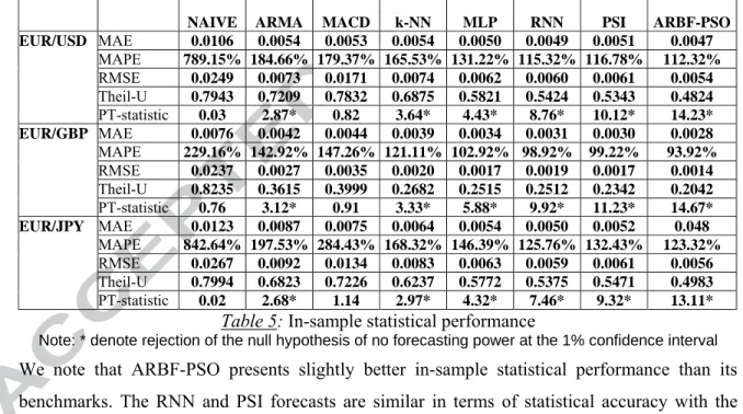
The in-sample statistical performance of our models is presented in table 5 below for the EUR/USD, the EUR/GBP and the EUR/JPY exchange rates. For the four error statistics retained (Root Mean Squared Error (RMSE), Mean Absolute Error (MAE), Mean Absolute Percentage Error (MAPE) and Theil-U) the lower the output, the better the forecasting accuracy of the model concerned. The Pesaran-Timmermann (PT) test (1992) examines whether the directional movements of the real and forecast values are in step with one another, or to put it another way, it checks how well rises and falls in the forecast value follow actual rises and falls. The null hypothesis is that the model under study has no power on forecasting the relevant exchange rate.

NAIVE ARMA MACD k-NN MLP RNN PSI ARBF-PSO

MAE 0.0106 0.0054 0.0053 0.0054 0.0050 0.0049 0.0051 0.0047 MAPE 789.15% 184.66% 179.37% 165.53% 131.22% 115.32% 116.78% 112.32% RMSE 0.0249 0.0073 0.0171 0.0074 0.0062 0.0060 0.0061 0.0054 Theil-U 0.7943 0.7209 0.7832 0.6875 0.5821 0.5424 0.5343 0.4824 EUR/USD PT-statistic 0.03 2.87* 0.82 3.64* 4.43* 8.76* 10.12* 14.23* MAE 0.0076 0.0042 0.0044 0.0039 0.0034 0.0031 0.0030 0.0028 MAPE 229.16% 142.92% 147.26% 121.11% 102.92% 98.92% 99.22% 93.92% RMSE 0.0237 0.0027 0.0035 0.0020 0.0017 0.0019 0.0017 0.0014 Theil-U 0.8235 0.3615 0.3999 0.2682 0.2515 0.2512 0.2342 0.2042 EUR/GBP PT-statistic 0.76 3.12* 0.91 3.33* 5.88* 9.92* 11.23* 14.67* MAE 0.0123 0.0087 0.0075 0.0064 0.0054 0.0050 0.0052 0.048 MAPE 842.64% 197.53% 284.43% 168.32% 146.39% 125.76% 132.43% 123.32% RMSE 0.0267 0.0092 0.0134 0.0083 0.0063 0.0059 0.0061 0.0056 Theil-U 0.7994 0.6823 0.7226 0.6237 0.5772 0.5375 0.5471 0.4983 EUR/JPY PT-statistic 0.02 2.68* 1.14 2.97* 4.32* 7.46* 9.32* 13.11*

Table 5: In-sample statistical performance

Note: * denote rejection of the null hypothesis of no forecasting power at the 1% confidence interval

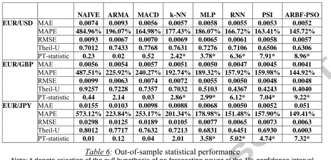
We note that ARBF-PSO presents slightly better in-sample statistical performance than its benchmarks. The RNN and PSI forecasts are similar in terms of statistical accuracy with the MLP presenting the third more accurate forecasts. The realizations of the statistical accuracy measures are considerably higher for our more traditional benchmarks, something that was expected based on their simplistic nature. On the other hand, the PT-statistics indicate that only our Naïve and MACD strategies are poor forecasts for the three exchange rates under study. In table 6 below we present the statistical performance of our models for the out-of-sample period.

(22)

NAIVE ARMA MACD k-NN MLP RNN PSI ARBF-PSO

MAE 0.0074 0.0093 0.0056 0.0057 0.0058 0.0055 0.0053 0.0052 MAPE 484.96% 196.07% 164.98% 177.43% 186.07% 166.72% 163.41% 145.72% RMSE 0.0093 0.0067 0.0070 0.0069 0.0065 0.0061 0.0058 0.0057 Theil-U 0.7012 0.7433 0.7768 0.7631 0.7276 0.7106 0.6506 0.6306 EUR/USD PT-statistic 0.23 0.02 0.52 2.42* 3.78* 6.36* 7.91* 8.96* MAE 0.0056 0.0054 0.0057 0.0051 0.0050 0.0047 0.0045 0.0041 MAPE 487.51% 225.92% 240.27% 192.74% 189.32% 157.92% 159.98% 144.92% RMSE 0.0099 0.0063 0.0074 0.0072 0.0055 0.0050 0.0048 0.0048 Theil-U 0.9257 0.7228 0.7357 0.7032 0.5103 0.4367 0.4243 0.4040 EUR/GBP PT-statistic 0.44 2.14 0.03 2.86* 2.99* 6.12* 7.04* 9.22* MAE 0.0155 0.0103 0.0098 0.0088 0.0068 0.0050 0.0052 0.051 MAPE 573.12% 223.84% 253.17% 201.34% 178.98% 151.48% 157.90% 149.41% RMSE 0.0298 0.0125 0.0189 0.0105 0.0077 0.0065 0.0073 0.0063 Theil-U 0.8012 0.7717 0.7632 0.7213 0.6831 0.6451 0.6930 0.6003 EUR/JPY PT-statistic 0.01 0.12 0.04 2.01 3.58* 5.02* 4.74* 7.32*

Table 6: Out-of-sample statistical performance

Note: * denote rejection of the null hypothesis of no forecasting power at the 1% confidence interval

From the results above, we note that ARBF-PSO retains its forecasting superiority in the out-of-sample sub-period for the statistical measures applied. Once more, the RNN and the PSI present the second best performance with MLP having the third best forecasts in terms of statistical accuracy. The PT statistics indicate that all our non linear models are good forecasts of the exchange rates under study except the k-NN model for the EUR/JPY series.

5.1.2 Diebold-Mariano Test

In order to test if our best model in terms of statistical measures produces forecasts that are statistically significant and superior to its counterparts, we apply the Diebold-Mariano (1995) statistic for predictive accuracy for both MSE and MAE loss functions (for more details on the test see Diebold and Mariano (1995)). The results of the Diebold-Mariano statistic, comparing the ARBF-PSO network with its benchmarks for the three exchange rates under study are summarized in the table 7 below.

Table 7: Diebold-Mariano Statistics

From the above table we note that the null hypothesis of equal predictive accuracy is rejected for all comparisons and for both loss functions at a 1% confidence interval, since all the test statistics are above the critical value of 2.33. Moreover, the statistical superiority of the

ARBF-NAIVE ARMA MACD k-NN MLP RNN PSI

MSE -8.456 -4.827 -5.542 -5.049 -4.214 -3.194 -3.224 EUR/USD MAE -9.143 -5.431 -6.281 -5.905 -5.104 -4.871 -4.523 MSE -8.812 -5.991 -7.840 -4.576 -4.402 -3.002 -3.344 EUR/GBP MAE -9.924 -6.214 -8.515 -5.385 -4.919 -3.461 -3.951 MSE -10.572 -6.718 -7.294 -5.751 -5.018 -3.851 -3.919 EUR/JPY MAE -10.917 -6.210 -7.821 -6.003 -5.891 -4.190 -4.387

(23)

PSO forecasts is confirmed as for both loss functions the realizations of the Diebold-Mariano (1995) statistic are negative9.

5.2 TRADING PERFOMANCE

5.2.1 Trading Strategy and Transaction Costs

In the previous section we evaluate our forecasts through a series of statistical accuracy measures and tests. However, statistical accuracy is not always synonymous of financial profitability. In financial applications, the practitioner’s utmost interest is in producing models that can be translated to profitable trades. It is therefore crucial to further examine our proposed model and evaluate its utility through a trading strategy. The trading strategy applied is to go or stay ‘long’ when the forecast return is above zero and go or stay ‘short’ when the forecast return is below zero. The ‘long’ and ‘short’ EUR/USD, EUR/GBP or EUR/JPY position is defined as buying and selling Euros at the current price respectively. When the forecast return is 0 we keep our position.

Transaction costs for a tradable amount, say USD 5-10 million, are about 1 pip per trade (one way) between market makers. But since we consider the EUR/USD, EUR/GBP and EUR/JPY time series as a series of middle rates, the transaction costs is one spread per round trip. For our dataset a cost of 1 pip is equivalent to an average cost of 0.007%, 0.012% and 0.008% per position for the EUR/USD, the EUR/GBP and the EUR/JPY respectively. Table 8 below presents the trading performance of our models in the in-sample sub-period.

NAIVE ARMA MACD k-NN MLP RNN PSI ARBF-PSO

Information Ratio (excluding costs) 0.01 0.89 0.29 1.73 1.91 2.46 3.15 3.74

Annualised Volatility (excluding costs) 10.56% 10.60% 10.59% 10.51% 10.58% 10.52% 10.49% 10.41%

Annualised Return (excluding costs) 0.11% 9.42% 3.07% 18.14% 20.23% 25.87% 33.02% 38.96%

Maximum Drawdown (excluding costs) -33.77% -13.76% -29.67% -31.74% -29.40% -21.38% -26.76% -25.57%

Positions Taken (annualised) 129 128 39 95 103 101 93 96

Transaction Costs (annualised) 0.90% 0.90% 0.27% 0.67% 0.72% 0.71% 0.65% 0.67%

Annualised Return (including costs) -0.79% 8.52% 2.80% 17.47% 19.51% 25.16% 32.37% 38.29% EUR/USD

Information Ratio (including costs) -0.08 0.80 0.26 1.66 1.84 2.39 3.09 3.68

Annualised Return (including costs) 2.62% 9.89% 3.19% 15.08% 18.87% 23.77% 25.35% 35.62% EUR/GBP

Information Ratio (including costs) 0.33 1.17 0.40 1.89 2.37 3.04 3.25 4.67

EUR/JPY

9_{We apply the Diebold-Mariano test to couples of forecasts (ARBF-PSO vs. another forecasting model). A}

negative realization of the Diebold-Mariano test statistic indicates that the first forecast (ARBF-PSO) is more accurate than the second forecast. The lower the negative value, the more accurate are the ARBF-PSOforecasts.

(24)

Annualised Return (including costs) 6.79% 9.91% 4.04% 16.08% 18.04% 26.40% 25.91% 30.03%

Information Ratio (including costs) 0.54 0.79 0.32 1.28 1.43 2.11 2.07 2.39

Table 8: In-sample trading performance

Clearly our ARBF-PSO network demonstrates a superior trading performance in terms of annualised return and information ratio for all exchange rates in the in-sample period. The PSI and the RNN produce the second and the third most profitable trades. In comparison with the statistical performance of our models for the same period, we note that although PSI and RNN present very close statistical forecasts, this is not always the case in trading terms. In general all our models are producing positive annualised returns except the naïve strategy for the EUR/USD something that was expected as all our models (except the naïve) were optimized during this period. In table 9 we present our results for the out-of-sample period.

NAIVE ARMA MACD k-NN MLP RNN PSI ARBF-PSO

Information Ratio (excluding costs) 0.07 -1.19 0.26 0.84 1.26 1.65 2.01 2.49

Annualised Return (excluding costs) 0.73% -12.55% 2.72% 8.88% 13.24% 17.27% 21.06% 25.93%

Annualised Return (including costs) -0.16% -13.31% 2.44% 7.96% 12.36% 16.40% 20.20% 25.10% EUR/USD

Information Ratio (including costs) -0.02 -1.26 0.23 0.75 1.17 1.56 1.93 2.41

Annualised Return (including costs) 3.22% 7.89% -0.11% 7.20% 10.85% 16.70% 17.33% 27.06% EUR/GBP

Information Ratio (including costs) 0.34 0.84 -0.01 0.77 1.16 1.79 1.86 2.92

Information Ratio (excluding costs) -0.81 0.10 -0.09 0.46 0.79 1.46 1.34 1.80

Annualised Return (excluding costs) -10.71% 1.30% -1.19% 6.11% 10.53% 19.36% 17.71% 23.96%

Transaction Costs (annualised) 1.09% 1.37% -0.34% 1.18% 1.17% 1.12% 1.22% 1.09%

Annualised Return (including costs) -11.80% -0.07% -1.53% 4.93% 9.36% 18.24% 16.49% 22.87% EUR/JPY

Information Ratio (including costs) -1.10 -0.01 -0.12 0.37 0.70 1.37 1.24 1.72

Table 9: Out-of-sample trading performance

We observe from the bold values of the above table that the ARBF-PSO confirms its trading superiority in the out-of-sample period. This is consistent with the superior statistical performance of our proposed methodology compared to its other NN and statistical benchmarks. A superiority that can be attributed to the proposed network algorithm that seems to excel in recognising the pattern of the two series under study compared to more traditional models. It is also worth noting that ARBF-PSO forecasts present a remarkably low maximum drawdown in

(25)

the out-of-sample period for all the three exchange rates under study. Thus the maximum potential losses of an investor are almost 3 or 4 times lower than the annualised profit in the out-of-sample period. Concerning our benchmarks models, we note that PSI and RNN present the second and the third best performance in terms of trading efficiency while our k-NN model has the fourth best performance with positive returns after transaction costs for all three exchange rates. The results of the more traditional models are mixed with the MACD for the EUR/USD and the naïve and ARMA for the EUR/GBP presenting slightly positive annualised returns after transaction costs.

Concerning our proposed fitness function of equation [9], the results from the statistical and trading evaluation of our NNs forecasts seem promising. Firstly we note that all our NNs present significant profits after transaction costs for all series under study in the out-of-sample period. Moreover, we did not note any large inconsistencies in our NNs statistical and trading performance for both exchange rates and sub-periods. Large inconsistencies could indicate that the training of our NNs is biased to either statistical accuracy or trading efficiency, something that could possibly lead to profitable in-sample forecasts but disastrous out-of-sample results. In the next section, we introduce a trading strategy to further increase the trading performance of our models.

5.3 LEVERAGE TO EXPLOIT HIGH INFORMATION RATIOS

In order to further improve the trading performance of our models we introduce a leverage based on GJR (1,1) one day ahead volatility forecasts10.The intuition of the strategy is to avoid trading when volatility is very high while at the same time exploiting days when the volatility is relatively low. As mentioned by Bertolini (2010), there are few papers on market-timing techniques for foreign exchange, with the notable exception of Dunis and Miao (2005). The opposition between market-timing techniques and time-varying leverage is only apparent as time-varying leverage can also be easily achieved by scaling position sizes inversely to recent risk measures behaviour.One of the primary restrictions of GARCH models is their symmetric response to positive and negative shocks. However, it has been argued that a negative shock to

10

We also explored a GARCH (1,1) model in forecasting volatility. Its statistical accuracy in the test sub-period in terms of the MAE, MAPE, RMSE and the Theil-U statistics is worse compared with GJR. Moreover, when we measure the utility of GARCH in terms of trading efficiency for our models withinthe context of our strategy in the test sub-period, our results in terms of annualised returns are slightly better with GJR for our models for all three exchange rates. However, we note that the use of the GJR model is quite puzzling for the series under studyas an exchange rate is a relative price (contrary to, say, a stock market price). So for example a 'negative shock to the EUR/USD' is in reality a negative shock to the EUR and at the same time a positive shock for the USD, and there is therefore no reason a priori why its impact should be larger than "a positive shock of the same magnitude" to the EUR/USD (i.e. a positive shock to the EUR and at the same time a negative shock for the USD), unless one makes

(26)

financial time series is likely to cause volatility to rise by more than a positive shock of the same magnitude (Bekaert and Wu (2000) and Brooks (2003)). A popular asymmetric formulation of GARCH which has an additional term to account for possible asymmetries is the GJR model, where the conditional variance is given by:

2 ₁ 1 2 1 2 1 2 − − − − + + + = t t t t t w au βσ γu I σ [21] where 2 t

σ and ut is the conditional variance and the error respectively at time t and It−1 =1 if 0

1 h −

t

u or 0 otherwise.

So we firstly forecast the one day ahead exchange rate volatility with a GJR (1,1) model in the test and validation sub-periods. Then, following Dunis and Miao (2005) we split these two periods into six sub-periods, ranging from periods with extremely low volatility to periods experiencing extremely high volatility. Periods with different volatility levels are classified in the following way: first the average (µ) difference between the actual volatility in day t and the forecast for day t+1 and its ‘volatility’ (measured in terms of standard deviation (ζ) are calculated; those periods where the difference is between µ plus one ζ are classified as ‘Lower High Vol. Periods’. Similarly, ‘Medium High Vol.’ (between µ + ζ and µ + 2 ζ) and ‘Extremely High Vol.’ (above µ + 2 ζ) periods can be defined. Periods with low volatility are also defined following the same 1 ζ and 2 ζ approach, but with a minus sign. For each sub-period a leverage is assigned starting with 0 for periods of extremely high volatility to a leverage of 2.5 for periods of extremely low volatility. Table 10 below presents the sub-periods and their relevant leverage factor.

Extremely

Low Vol. Medium Low Vol. Lower Low Vol. Lower High Vol. Medium High Vol. Extremely High Vol.

Leverage 2.5 2 1.5 1 0.5 0

Table 10: Sub-periods and leverage factor

The parameters of our strategy (µ and ζ) are updated every three months by rolling forward the estimation period. So for example, for the first three months of our validation period, µ and ζ are computed based on the twenty four months of the test sub-period. For the following three months, the two parameters are computed based on the last fifteen months of our test sub-period and the first three of the validation sub-period. The cost of leverage (interest payments for the additional capital) is calculated at 1.75% p.a. (that is 0.0069% per trading day11). This leverage

the assumption that financial markets have a negative bias against the EUR (something that might explain the superior perfomance of GJR than GARCH in our study).

11_{The interest costs are calculated by considering a 1.75% interest rate p.a. (the Euribor rate at the time of}

calculation) divided by 252 trading days. In reality, leverage costs also apply during non-trading days so that we should calculate the interest costs using 360 days per year. But for the sake of simplicity, we use the approximation

(27)

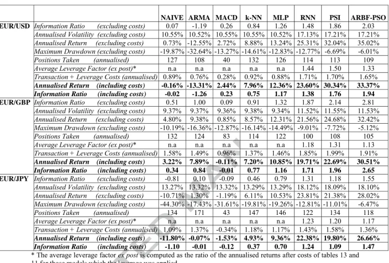
is applied to the models that have achieved an in-sample information ratio of at least 2 and, as such, would have been candidates for leveraging out-of-sample. Our final results are presented in table 11.

NAIVE ARMA MACD k-NN MLP RNN PSI ARBF-PSO

Information Ratio (excluding costs) 0.07 -1.19 0.26 0.84 1.26 1.48 1.86 2.03

Annualised Return (excluding costs) 0.73% -12.55% 2.72% 8.88% 13.24% 25.31% 32.04% 35.02%

Average Leverage Factor (ex post)* n.a n.a n.a n.a n.a 1.44 1.50 1.33

Transaction + Leverage Costs (annualised) 0.89% 0.76% 0.28% 0.92% 0.88% 1.71% 1.70% 1.65%

Annualised Return (including costs) -0.16% -13.31% 2.44% 7.96% 12.36% 23.60% 30.34% 33.37% EUR/USD

Information Ratio (including costs) -0.02 -1.26 0.23 0.75 1.17 1.38 1.76 1.94

Annualised Return (excluding costs) 4.80% 9