An empirical evaluation of classification algorithms for fault prediction in open source projects

(1)

An empirical evaluation of classification algorithms

for fault prediction in open source projects

Arvinder Kaur, Inderpreet Kaur

*

Dept: CSE/IT, University School of Information and Communication Technology, Guru Gobind Singh Indraprastha University, Dwarka, New Delhi 110078, India

Received 23 September 2015; revised 17 March 2016; accepted 8 April 2016

KEYWORDS Metrics; Fault prediction;

Receiver Operating Charac-teristics Analysis;

Machine learning; Nimenyi test

Abstract Creating software with high quality has become difﬁcult these days with the fact that size and complexity of the developed software is high. Predicting the quality of software in early phases helps to reduce testing resources. Various statistical and machine learning techniques are used for prediction of the quality of the software. In this paper, six machine learning models have been used for software quality prediction on ﬁve open source software. Varieties of metrics have been evaluated for the software including C & K, Henderson & Sellers, McCabe etc. Results show that Random Forest and Bagging produce good results while Naı¨ve Bayes is least preferable for prediction. Ó2016 The Authors. Production and hosting by Elsevier B.V. on behalf of King Saud University. This is an open access article under the CC BY-NC-ND license (http://creativecommons.org/licenses/by-nc-nd/4.0/).

1. Introduction

Building high quality software with limited quality assurance budgets has become difﬁcult. Various Software prediction models are used these days to learn fault predictors from soft-ware metrics. Softsoft-ware fault prediction, prior to the release of software helps in veriﬁcation and validation activity and allocate the limited resources to modules which are predicted to be fault prone. Early and accurate fault prediction is a better approach for reducing testing efforts. Study (Mahanti and

Antony, 2005) shows that software companies spend 50–80 percent of their software development effort on testing.

If fault prone modules are known in advance, review, anal-ysis and testing efforts can be concentrated on those modules. Early detection of fault prone modules in the software life cycle has become one of the important goals of fault prediction because, earlier the detection of fault, the cheaper it is to cor-rect it. Boehm and Papaccio advised ﬁxing the fault early in the life cycle can make it cheaper by a factor of 50–200 (Boehm and Papaccio, 1988). Reliability of delivered products can be ensured using software quality models.

Software quality estimation using various classiﬁers is per-formed where input is some metrics and output is quality attri-butes. Empirical Study of these classiﬁers, aids in judgment of the quality of software being developed.

Various techniques have been suggested to deal with defect prediction which include categorizing modules, represented by a set of software metrics or code attributes into fault prone and non-fault-prone by means of classiﬁcation model derived from data as per the previously developed projects (Schneidewind, * Corresponding author.

E-mail addresses:[email protected](A. Kaur),kaur. [email protected](I. Kaur).

Peer review under responsibility of King Saud University.

Production and hosting by Elsevier

Journal of King Saud University – Computer and Information Sciences (2016)xxx, xxx–xxx

King Saud University

Journal of King Saud University –

Computer and Information Sciences

www.ksu.edu.sa www.sciencedirect.com

http://dx.doi.org/10.1016/j.jksuci.2016.04.002

1319-1578Ó2016 The Authors. Production and hosting by Elsevier B.V. on behalf of King Saud University. This is an open access article under the CC BY-NC-ND license (http://creativecommons.org/licenses/by-nc-nd/4.0/).

Please cite this article in press as: Kaur, A., Kaur, I. An empirical evaluation of classification algorithms for fault prediction in open source projects. Journal of King Saud University – Computer and Information Sciences (2016),http://dx.doi.org/10.1016/j.jksuci.2016.04.002

(2)

1992).This also includes code metrics (e.g., lines of code, com-plexity) (Li and Henry, 1993; Chidamber and Kemerer, 1994; Lorenz and Kidd, 1994; McCabe and Associates, 1994; Basili et al., 1996; Henderson-Sellers, 1996; Ohlsson and Alberg, 1996; Briand et al., 1999; El Emam et al., 2001a,b,c; Gyimothy et al., 2005; Aggarwal et al., 2006; Nagappan and Ball, 2005; Nagappan et al., 2006), Process metrics (e.g., num-ber of changes, recent activity) (Hassan, 2009; Moser et al., 2008; Bernstien et al., 2007), or previous defects (Kim et al., 2007; Ostrand et al., 2005; Hassan and Holt, 2005). The decision is still out on the relative performance of these approaches. Most of them have been judged were compared to only few other approaches. In addition, a signiﬁcant portion of the evaluations cannot be reproduced since the data used for their evaluation came from commercial systems and are not available for public consumption. In some cases, researchers concluded differently: For example, in the case of size metrics, Gyimothy et al. reported good results (2005), as opposed to the ﬁndings ofFenton and Ohlsson (2000).

Various types of classifiers have been applied to this task, including statistical procedures (Basili et al., 1996; Khoshgoftaar and Seliya, 2004), tree-based methods (Selby and Porter, 1988; Porter and Selby, 1990; Khoshgoftaar et al., 2000; Guo et al., 2004; Menzies et al., 2004), neural net-works (Khoshgoftaar et al., 1995; Khoshgoftaar et al., 1997), and analogy-based approaches (Khoshgoftaar et al., 2000; El Emam et al., 2001a,b,c; Khoshgoftaar and Seliya, 2003). How-ever, as noted in (Myrtveit and Stensrud, 1999; Shepperd and Kadoda, 2001; Myrtveit et al., 2005) results regarding the superiority of one method over another or the usefulness of metric-based classification in general are not always consistent across different studies. Therefore, ‘‘There is a need to develop more reliable research procedures before we can have confidence in the conclusion of comparative studies of soft-ware prediction models”(Myrtveit et al., 2005).

Various classiﬁcation algorithms have been applied to a variety of data sets. Different experimental setup results limit the ability to understand classiﬁer’s pros and cons. A modeling technique is good if it is able to perform well on all or at least most of them. To simplify model comparison, appropriate and consistent performance measures should be considered.

Evaluating the performance of various approaches is subject to discussion. While some use Binary classiﬁcation (i.e. predicting if a given entity is a buggy or not) others predict by prioritizing components with most defects. In this paper, the binary classiﬁcation technique is used which has been eval-uated on the basis of the ROC, lift chart and other statistical parameters.

The datasets used in this work are open source java projects: PMD, EMMA, Find Bugs, Trove and Dr Java. Open source projects are different from Industrial projects. Open source software, is preferred for research as results of these can be compared and repetition of validation can be per-formed. Open source projects foster more creativity and have fewer defects as defects are found and ﬁxed rapidly. (Paulson et al., 2004).

In this paper, the six well-known classification algorithms have been used Classifiers selected are Random Forest, Naive Bayes, Bagging, J48, logistic regression and IB1. These six classifiers have been chosen for the current study as previous studies indicate that these classifiers provide better than aver-age performance in software fault prediction (Menzies et al.,

2007a,b; Jiang et al., 2008). Many studies have used insufﬁ-cient performance metrics which do not show enough level of details for future comparison. Therefore, the objectives of this paper include:

1. To compare models for fault prediction on open source software on the basis of

(i) Performance measures including accuracy, sensitiv-ity, speciﬁcsensitiv-ity, Precision, G-mean, F-measure, J_coefﬁcient.

(ii) Graphical methods which include ROC curve, Precision Recall curve, Cost curves and Lift charts. (iii) Non parametric Freidman test followed by the post

hoc Nimenyi test.

2. To compare the results of open source software projects with industrial data sets.

The paper is organized as follows: Section 2 presents the overview of Related Work. Section 3 describes the Research methodology along with datasets and metrics used for the clas-siﬁer selection. Section 4 represents the model evaluation tech-niques, which includes comparison of numerical performance indices, Graphical evaluation techniques and statistical test performed. Section 5 consists of the analysis performed on each of the data sets taken in this work. Section 6 discusses the guidelines for selecting the best model followed by conclu-sions in section 7.

2. Related work

Basili et al. (1996)found that several of the (Chidamber and Kemerer, 1994) metrics were associated with fault proneness based on a study of eight medium-sized systems, developed by students.

Tang et al. (1999)analysed (Chidamber and Kemerer, 1994) OO metrics suite on three industrial applications developed in C++. They found none of the metrics examined to be signif-icant except RFC and WMC.

Briand et al. (2000)have extracted 49 metrics to identify a suitable model for predicting fault proneness of classes. The system under investigation was a medium sized C++ soft-ware system developed by undergraduate/graduate students. There were eight systems under study, consisting a total of 180 classes. They used univariate and multivariate analyses to ﬁnd the individual and combined impact of OO metrics and fault proneness. The results showed all metrics except NOC (which was found related to fault proneness in an inverse manner) to be signiﬁcant predictors of fault proneness.

El Emam et al., 2001a,b,cexamined a large telecommunica-tion applicatelecommunica-tion developed in C++ and found that class size i.e. SLOC has a confused effect of most OO metrics on faults. Another study byBriand and Wust (2001)used a commer-cial system consisting of 83 classes. They found the DIT metric related to fault proneness in an inverse manner and NOC met-ric to be an insigniﬁcant predictor of fault proneness.

Yu et al. (2002)choose eight metrics and they examined the relationship between these metrics and the fault proneness. The subject system was the client side of a large network service management system developed by three professional software engineers. It was written in Java, and consisted of

(3)

123 classes and around 34,000 lines of code. First, they exam-ined the correlation among the metrics and found four highly correlated subsets. Then, they used univariate analysis to ﬁnd out which metrics could detect faults and whichKhoshgoftaar and Seliya (2004)in their experiments suggested that a module which is currently in development is likely to be fault prone if it has similar or same characteristics as of the faulty module measured by software metric that has been developed or released earlier in the same environment. So, historical data guide us to predict fault proneness.

Lessmann et al. (2008)in their studies proposed a frame-work for comparative software defect prediction experiments which was applied in large scale empirical comparison of 22 classifiers over 10 datasets from NASA MDP. Advisable degree of predictive accuracy was observed and thus supports the view that metric based classification is useful. And also that no significant performance differences could be detected amongst top 17 classifiers.

Malhotra and Jain (2012)studied the relationship between object oriented metrics and fault proneness using logistic regression method. Receiver Operating Characteristic (ROC) Analysis was used and performance of predicted models is thus evaluated based on ROC.

In other studiesMalhotra (2014), a statistical model derived from logistic regression was used to calculate the threshold val-ues of object oriented, Chidamber and Kemerer metrics. Using threshold values, they have shown threshold effects at various risk levels and validated the use of these thresholds on a public domain, proprietary dataset, KC1 obtained from NASA and two open source, promise datasets, IVY and JEdit using vari-ous machine learning methods and data mining classiﬁers. Interproject validation was also carried out on three different open source datasets, Ant and Tomcat and Sakura. Their results showed that the proposed threshold methodology works well for the projects of similar nature or having similar characteristics.

Okutan and Yildiz (2012)used Bayesian networks to deter-mine the probabilistic inﬂuential relationships among software metrics and defect proneness. They used two more metrics in addition to the metrics used in Promise data repository, num-ber of developers (NOD) and source code quality (LOCQ). They used 9 open source Promise data repository data sets. Their results showed that response for class (RFC), lines of code (LOC) and lack of coding quality (LOCQ) are most effec-tive metrics whereas coupling objects (CBO), weighted method per class (WMC) and lack of cohesion of methods (LCOM) are less effective metrics on defect proneness.

The difference between their work and our work is that their study is applied on industrial data sets whereas our work is applied on open source projects. This comparative study would help to determine whether the results obtained from industrial datasets are applicable to open source datasets or whether open source projects give different results. Open source projects are developed entirely in different environment than that of industrial datasets. Anyone can view, edit or com-pare the codes of open source with other projects while indus-trial datasets pose this limitation. Bugs encountered are well tracked in open source projects as well as industrial projects but will not be available to public in industrial datasets (Paulson et al., 2004).

Yeresime et al. (2014)studied application of linear regres-sion, logistic regresregres-sion, and artiﬁcial neural network methods for software fault prediction on CK metrics. Here, fault is con-sidered as dependent variable and CK metric suite as indepen-dent variables. These statistical models were applied on case study for Apache integration framework (AIF) version 1.6. Their results point out importance of weighted method per class (WMC) metric for fault classiﬁcation, and hybrid approach of radial basis function network obtained better fault prediction rate when compared with other three neural network models.

Research carried out by Jiang et al. (2008) used NASA MDP industrial datasets KC1, KC2, KC4, JM1, PC1, PC5, CM1 and MC2 to evaluate the best amongst the given classiﬁer models. Their studies were based on comparison of perfor-mance indices, graphical evaluations and statistical tests for model selection. This paper follows the framework of analysis of data as used by Jiang et al. and is in support of the studies carried out byJiang et al. (2008).

The difference between their work and our work is that their study is applied on industrial data sets, whereas our work is applied on open source projects. This comparative study would help to determine whether the results obtained from industrial datasets are applicable to open source datasets or whether open source projects give different results. Open source projects are developed entirely in a different environ-ment than that of industrial datasets. Anyone can view, edit or compare the codes of open source with other projects while industrial datasets pose this limitation. Bugs encountered are well tracked in open source projects as well as industrial pro-jects, but will not be available to public in industrial datasets (Paulson et al., 2004).

3. Research methodology

Fault proneness is deﬁned as the probability of fault detection in a class (Briand et al., 2000; Pai, 2007; Aggarwal et al., 2009). Open source java projects have been used in this work. Open source software is freely available software so the results of these can be compared and repetition of validation can be per-formed. Non parametric statistical Friedman test followed by Nimenyi test is performed for selection of the best classiﬁer amongst all.

3.1. Empirical data collection

This study uses open source java projects. Their bug infor-mation has been gathered from the source forge, where the bug tracker keeps the status of Bugs (open/closed). Source Forge is dedicated to make open source projects successful. SourceForge.net is owned and operated by Geeknet Media and is a Dice Holdings, Inc. company. The data sets are made for open source java projects which include (PMD), Find Bugs, EMMA, Trove and Dr Java. Their Bugs are col-lected from the SOURCEFORGE (an open source bug tracker) and data without Bugs have been collected from the source code java ﬁles. Using those java ﬁles, various metrics are calculated with the CKJM tool which gives us metrics including WMC, DIT, NOC, RFC, CBO, LCOM,

Evaluation of classiﬁcation algorithms for fault prediction 3

(4)

LCOM3, IC, CBM, AMC, NPM, DAM, MOA, MFA, CC, LOC, CA, CE.

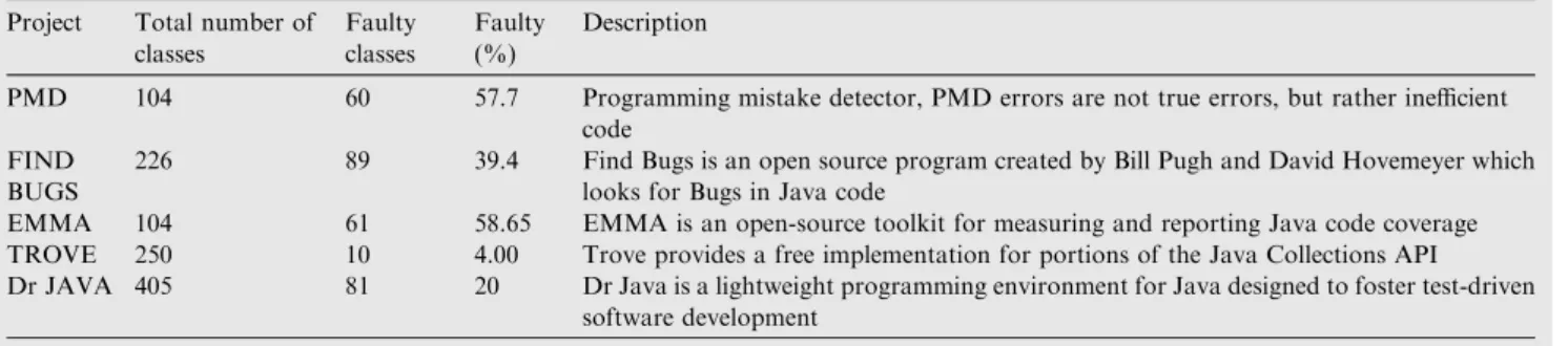
Table 1lists the projects used with their description.

3.2. Metrics evaluated

Twenty software metrics have been measured on these data sets. The metrics chosen are the ones which are most com-monly used for object oriented software. All C & K metrics and more metrics like Henderson-Sellers and QMOOD have been taken into account. TheTable 2 represents the descrip-tion of the metrics used. CKJM extended tool has been used to evaluate the metrics of the open source java projects.

In this paper, the six well-known classification algorithms have been used Classifiers selected are Random Forest, Naive Bayes, Bagging, J48, logistic regression and IB1 These six clas-sifiers have been chosen for the current study as previous stud-ies indicate that these classifiers provide better than average performance in software fault prediction (Boehm and Papaccio, 1988). The comparison of classifiers is based on

performance indices, graphical methods and statistical tests have been done. It was seen that no one measure is sufficient to give insight on the best classifier selection, rather the selec-tion should be based on the project cost involved and specific project needs (Jiang et al., 2008). The Waikato Environment for Knowledge Analysis (Weka) has been used for implemen-tation of the classifiers selected.

4. Model evaluation

The models used are compared based on numerical perfor-mance indices such as accuracy, sensitivity, specificity, Preci-sion, G-mean, F-measure and J_coefficient. Graphical evaluation techniques used includes the ROC, Precision Recall (PR) Curve, Lift charts and Cost curve. Statistical tests are required to select the best model from given classifiers. Empir-ical validation of machine learning methods is needed to verify the potentiality of machine learning algorithms. The results collected from these empirical studies are considered to be powerful support for testing any given hypothesis.

Table 1 Projects description. Project Total number of

classes Faulty classes Faulty (%) Description

PMD 104 60 57.7 Programming mistake detector, PMD errors are not true errors, but rather ineﬃcient code

FIND BUGS

226 89 39.4 Find Bugs is an open source program created by Bill Pugh and David Hovemeyer which looks for Bugs in Java code

EMMA 104 61 58.65 EMMA is an open-source toolkit for measuring and reporting Java code coverage TROVE 250 10 4.00 Trove provides a free implementation for portions of the Java Collections API Dr JAVA 405 81 20 Dr Java is a lightweight programming environment for Java designed to foster test-driven

software development

Table 2 Metrics description.

Metrics Description Source

WMC Weighted methods per class (NOM: number of methods in the QMOOD metric suite) C & K

DIT Depth of inheritance tree C & K

NOC Number of children C & K

RFC Response for a class C & K

CBO Coupling between object classes C & K

LCOM Lack of cohesion in methods C & K

LCOM3 LCOM lack of cohesion in methods is a normalized version of the Chidamber and Kemerer’s LCOM metric and its value varies between 0 and 2

Henderson-Sellers

IC Inheritance coupling Quality oriented extension to C &

amp K metric suite

CBM Coupling between methods Quality oriented extension to C &

amp K metric suite

AMC Average method complexity Quality oriented extension to C &

amp K metric suite NPM Number of public methods for a class (also called as CIS: class interface size) QMOOD

DAM Data access metric QMOOD

MOA Measure of aggregation QMOOD

MFA Measure of functional abstraction QMOOD

CAM Cohesion among methods of class QMOOD

CC Cyclomatic complexity McCabe’s

LOC Lines of code McCabe’s

Ca Aﬀerent coupling Martin’s metrics

(5)

4.1. Numerical performance evaluation indices

The most commonly used performance measures have been described. This section provides information related to their strengths and weakness. The indices have been calculated based on the confusion matrix given by the classifier. A confu-sion matrix (Provost and Kohavi, 1998) contains information about actual and predicted classifications done by a classifica-tion system. Performance of such systems is commonly evalu-ated using the data in the matrix. The following table shows the confusion matrix for a two class classifier.

The entries in the confusion matrix have the following meaning in the context of our study:

ais the number of correct predictions that an instance is negative,

bis the number ofincorrectpredictions that an instance is positive,

cis the number ofincorrectof predictions that an instance negative, and

dis the number of correct predictions that an instance is positive.

4.1.1. Accuracy

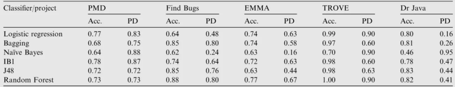
Accuracy is the proportion of the total number of predictions that are correct. It doesn’t take into account the data distribu-tion and cost informadistribu-tion (Jiang et al., 2008).The Probability of Detection (PD) is a proportion of positive cases that are cor-rectly identiﬁed (Jiang et al., 2008) (seeTable 3).

Table 4provides the accuracy and probability of detection rates for five projects: PMD, FIND BUGS, EMMA, TROVE and Dr JAVA. It can be seen from the results that the highest accuracy is followed with the lowest detection rate. This lower detection rate means many faulty modules would be classified as fault free, which can result into serious failures. Hence, one cannot rely on the accuracy measure only for performance measurement of the classifier.

As faulty modules are likely to represent a minority of mod-ules in the dataset, so the accuracy measure could provide a wrong impression.

4.1.2. Sensitivity, specificity and precision

The Recall or True Positive rate (TP) or Sensitivity is the pro-portion of positive cases (faulty modules) that were correctly identiﬁed. It is also termed as Probability of Detection (PD) (Jiang et al., 2008). The techniques which produce low PD are poor fault predictors.

Specificity is the proportion of correctly identified negative cases (fault free modules) .The Probability of False alarm (PF) is a proportion of negative cases that are classified erroneously (Jiang et al., 2008).

So;PF¼1Specificity:

The low value of Speciﬁcity will increase the veriﬁcation and validation of fault free modules, as they would be incor-rectly marked as faulty, thus increasing the cost and time required for the testing of these modules.

The precision (P) is the proportion of the predicted positive cases that were correct (Jiang et al., 2008). Table 5 presents these values for open source projects taken in this study. There always exists a compromise between precision, sensitivity and speciﬁcity. Because sensitivity takes care of faulty modules and speciﬁcity will monitor fault free modules, the perfor-mance of prediction models based on these measures will be one sided. So comparing models based on only these measures cannot provide good evaluation of fault prediction.

4.1.3. G-mean, F-measure and J_coefficient

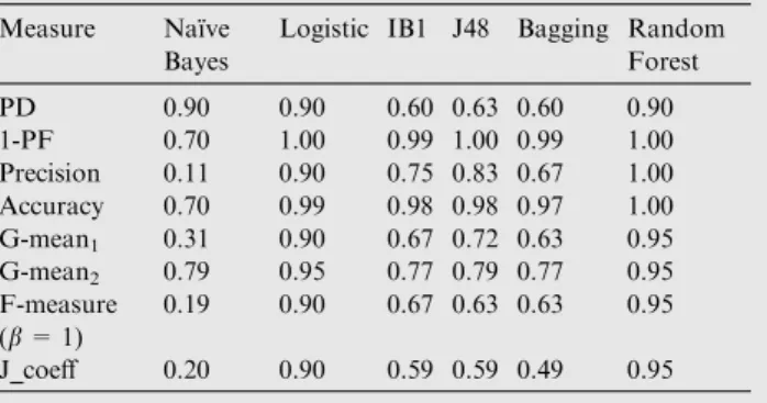
Compared to accuracy, Geometric mean (McCabe and Associates, 1994), F-measure (Kubat et al., 1998) and J_coef-ficient (Lewis and Gale, 1994) give better model performance. Two G-mean indices are defined. G-mean1is the square root of the product of sensitivity and precision. G-mean2is the square root of the product of sensitivity and specificity. In software fault prediction, it is important to identify more faulty modules which mean a high probability of detection is needed. So if two classifiers predict with a same or similar PD, the one with higher specificity would be preferred. Precision defines the actual faulty modules amongst the predicted fault modules. G-mean1¼ ffiffiffiffiffiffiffiffiffiffiffiffiffiffiffiffiffiffiffiffiffiffiffiffiffiffiffiffiffiffiffi PDPrecision p ðiÞ G-mean2¼ ffiffiffiffiffiffiffiffiffiffiffiffiffiffiffiffiffiffiffiffiffiffiffiffiffiffiffiffiffiffiffiffiffi PDSpecificity p ðiiÞ F-measure¼ðb 2_þ₁_Þ_Precision_PD b2 PrecisionþPD ðiiiÞ

J coeff¼SensitivityþSpecificity1

¼PD1þSpecificity

¼PDPF

ðivÞ

Table 3 Confusion matrix.

Predicted

Negative Positive

Actual Negative a b

Positive c d

Table 4 Accuracy and PD for projects taken.

Classiﬁer/project PMD Find Bugs EMMA TROVE Dr Java

Acc. PD Acc. PD Acc. PD Acc. PD Acc. PD

Logistic regression 0.77 0.83 0.64 0.48 0.74 0.63 0.99 0.90 0.80 0.16 Bagging 0.68 0.75 0.85 0.80 0.74 0.58 0.97 0.60 0.81 0.26 Naı¨ve Bayes 0.64 0.88 0.62 0.24 0.63 0.16 0.70 0.90 0.46 0.95 IB1 0.78 0.87 0.74 0.64 0.72 0.63 0.98 0.60 0.78 0.47 J48 0.72 0.72 0.85 0.76 0.63 0.44 0.98 0.63 0.83 0.44 Random Forest 0.73 0.73 0.88 0.80 0.77 0.67 1.00 0.90 0.82 0.41

(6)

F-measure provides better ﬂexibility which includes the weight factor b .This weight factor helps to manipulate the cost assigned to PD and precision. Factor b can have any non negative value. Setting it to 1 provides equal weight to PD and precision. Higher the value of b, higher the weight assigned to PD.

Youden (1950)proposed the J_coeff to evaluate models in medical sciences. El-Emam were first to use it to compare clas-sifiers (El El Emam et al., 2001a,b,c). When J_coeff is 0,PD¼PF, so these classifiers are not of much help. When J coeff>0, PD>PF, which means the classifier is good. Therefore, for if the J coeff¼1 it represents perfect classifica-tion while J coeff¼ 1 means the bad case.Table 6lists the three measures of projects taken.

These three measures are better than accuracy measure. A model which is able to detect more fault prone modules is good. When the project is of a low budget, a smaller number of faulty prone modules with a low false alarm rate would be desirable. In such conditions, the ﬂexibility of G-mean, J_coeff and F-measure would help in better performance eval-uation. These measures are preferable in evaluating software fault prediction models as the cost associated with misclassify-ing a fault prone module is higher than misclassifymisclassify-ing it as non fault prone module, which implies some wastage of resources in veriﬁcation activities.

4.2. Graphical methods

Different graphical methods available for performance evalua-tion include:

Receiver Operating Characteristic (ROC) curve

Precision and Recall curve

Cost curve

Lift chart.

Studies indicate that cost curves are novel in software engi-neering literature. All these graphs are derived from confusion matrix. ROC and Lift chart are closely related (Ling and Li, 1998). Each curve depicts a different view of classiﬁcation performance.

4.2.1. ROC curve

ROC is a curve formed by PF, PD pairs. It is a more general way for classiﬁer’s performance measurement than the numer-ical indices (Yousef et al., 2004). It provides the better compro-mise between PD and PF.

Area under the ROC curve (AUC) is commonly used for performance evaluation. The entire area is of no interest, for example, the area where PD is low or where the PF is high and regions with high PF and low PD are indicators of poor performance. Only the region which has low PF and high PD is likely to have some impact on the classifier performance. The advantages of the ROC analysis are its robustness toward imbalanced class distributions and to varying and sym-metric misclassification costs (Yousef et al., 2004). Therefore, it is particularly well suited for software defect prediction tasks which naturally exhibit these characteristics (Khoshgoftaar and Seliya, 2004; Menzies et al., 2007a,b). To compare differ-ent classifiers, their respective ROC curves are drawn in ROC space.Fig. 1provides an example of three classifiers, C1, C2,

and C3. C1 is a dominating classiﬁer because its ROC curve is always above that of its competitors, i.e., it achieves a higher TP rate for all FP rates.

The AUC has the potential to signiﬁcantly improve conver-gence across empirical experiments in software defect predic-tion because it separates predictive performance from operating conditions, i.e., class and cost distributions, and thus represents a general measure of predictiveness.

The importance of such a general indicator in comparative experiments is reinforced considering the discussion following Menzies et al.’s paper (Menzies et al., 2007a,b).That discusses whether the accuracy of their models is or is not sufficient for practical applications and whether the method A is or is not better than the method B (Menzies et al., 2007a,b). Further-more, the AUC has a clear statistical interpretation: It mea-sures the probability that a classifier ranks a randomly chosen fp module higher than a randomly chosen nfp module, which is equivalent to the Wilcoxon test of ranks El Emam et al., 2001c. Consequently, any classifier achieving AUC well above 0.5 is demonstrably effective for identifying fp modules and gives valuable advice as to which modules should receive particular attention in software testing.

ROC curves for six classiﬁers used for PMD dataset is rep-resented in theFig. 1. Graph shows that Random Forest tech-nique provides the best ROC amongst all the six classiﬁers.

4.2.2. Precision–Recall curve

PR curve may help in differentiating between algorithms used with better visualization than ROC. Here Recall is represented on x-axis and Precision on y-axis. Example for PR curve is shown inFig. 2for dataset Find Bugs.

Our area of interest is where precision and Recall both are high, that makes Random Forest technique better as it outper-forms the Bagging technique in that particular region.

So in cases where ROC isn’t able to provide the differences amongst classiﬁers, PR curve can be of good use.

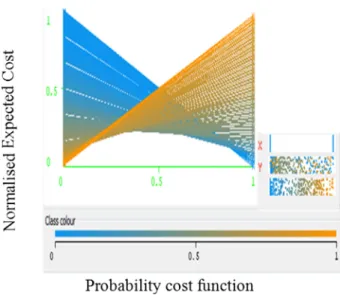
4.2.3. Cost curve

ROC and PR curve don’t consider the cost of misclassification. Adams and Hand (1999) defined the loss difference plots to take the advantage of the misclassification cost ratio.

Drummond and Holte (2006) proposed the cost curve, which allows describing the classiﬁer’s performance based on the cost of misclassiﬁcation.

Cost curves are generated by drawing a straight line con-necting points (0, PF) and (1, 1-PD). The lower part is formed by connecting all the intersection points from left to right. Cost curve for Find Bugs using Random Forest and logistic regres-sion is shown inFigs. 3 and 4.

ROC and PR curves aim at maximizing the area under the curve whereas the cost curves minimize the misclassification cost, that is minimize the lower envelope area. Smaller the areas in the lower envelope better the performance of the clas-sifier and hence better cost-benefit ratio.

During comparison of classiﬁers, it is better to plot all these curves because they provide complementary facts for the clas-siﬁer selection.

4.2.4. Lift chart

Due to limited resources and time constraints for veriﬁcation and validation activities, the efﬁcient utilization of resources

(7)

Table 5 Sensitivity, speciﬁcity and precision values for datasets taken.

Classiﬁer/project PMD Find Bugs EMMA TROVE Dr Java

Sensitivity Specificity Precision Sensitivity Specificity Precision Sensitivity Specificity Precision Sensitivity Specificity Precision Sensitivity Specificity Precision

Logistic regression 0.83 0.68 0.78 0.48 0.80 0.70 0.63 0.82 0.71 0.90 1.00 0.90 0.16 0.96 0.50 Bagging 0.75 0.59 0.71 0.80 0.89 0.83 0.58 0.85 0.74 0.60 0.99 0.67 0.26 0.95 0.58 Naı¨ve Bayes 0.88 0.32 0.64 0.24 0.87 0.54 0.16 0.97 0.78 0.90 0.70 0.11 0.95 0.34 0.26 IB1 0.87 0.66 0.78 0.64 0.81 0.69 0.63 0.79 0.68 0.60 0.99 0.75 0.47 0.86 0.46 J48 0.72 0.73 0.78 0.76 0.91 0.85 0.44 0.75 0.56 0.63 1.00 0.83 0.44 0.93 0.61 Random Forest 0.73 0.73 0.79 0.80 0.93 0.89 0.67 0.84 0.74 0.90 1.00 1.00 0.41 0.93 0.58

Table 6 The value of three measures for the projects.

Classiﬁer/ project

PMD Find Bugs EMMA TROVE Dr JAVA

G-mean1 G-mean2 F-measure G-mean1 G-mean2 F-measure G-mean1 G-mean2 F-measure G-mean1 G-mean2 F-measure G-mean1 G-mean2 F-measure

Logistic regression 0.81 0.75 0.81 0.58 0.62 0.57 0.67 0.72 0.67 0.9 0.95 0.90 0.28 0.39 0.24 Bagging 0.73 0.66 0.73 0.81 0.84 0.81 0.65 0.70 0.65 0.63 0.77 0.63 0.38 0.49 0.36 Naı¨ve Bayes 0.75 0.53 0.74 0.36 0.46 0.33 0.35 0.39 0.27 0.31 0.79 0.19 0.49 0.57 0.41 IB1 0.82 0.76 0.82 0.66 0.72 0.66 0.65 0.71 0.65 0.67 0.77 0.67 0.46 0.64 0.46 J48 0.75 0.72 0.75 0.80 0.83 0.80 0.49 0.57 0.49 0.72 0.79 0.63 0.52 0.64 0.51 Random Forest 0.76 0.73 0.76 0.84 0.86 0.84 0.70 0.75 0.71 0.95 0.95 0.95 0.49 0.62 0.48 Evaluation of classiﬁcation algorithms for fault prediction 7 Please cite this article in press as: Kaur, A., Kaur, I. An empiri cal evaluation of classi fication algorithms for fault prediction in open source proje cts. Journ al of King Saud University – Computer and Information Sciences (2016), http://dx.doi.o rg/10.1016/ j.jksuci.2016. 04.002

(8)

to achieve the best quality improvement is a challenge. Lift chart (Witten and Frank, 2005) also known as Alberg Diagram (Khoshgoftaar and Seliya, 2004; Ostrand et al., 2005; Ohlsson and Alberg, 1996; Ohlsson et al., 1997) is another performance evaluation measure. Lift is measurement of how efficiently a classifier detects fault prone modules. It evaluates the ratio of correctly identified faulty modules with and without predictive model.

In the lift chart, the x-axis represents the percentage of modules considered and y-axis represents the corresponding detection rate. The lift chart includes a baseline and a lift curve. The greater the area between the lift and baseline is, the better the performance of the classiﬁer.

Lift chart for dataset FIND BUGS with top three classiﬁers logistic regression, Bagging and Random Forest is shown in Fig. 5.

4.3. Statistical comparisons of models

Performance measures are not adequate for comparison of classiﬁers; statistical conclusions are required to actually compare the classiﬁers (Conover, 1999; Siegel, 1956).

The goal is to select the best technique amongst given techniques. The hypothesis made is:

Ho: There is no difference in performance of six classiﬁers.

Figure 1 ROC’s for classiﬁers used in PMD.

Figure 2 Precision Recall curve in Find Bugs.

Figure 3 Cost curve for Find Bugs using Random Forest.

Figure 4 Cost curve for Find Bugs using Logistic.

(9)

HA: At least one classiﬁer performs signiﬁcantly better than others.

Rejection of the null hypothesis can be preceded by the post hoc test.Demsar (2006)recommends Friedman test followed by corresponding post-hoc Nemenyi test if more than two clas-siﬁers are taken over multiple datasets. Demsar recommends these tests as they are less strict on the data. But non paramet-ric tests do not utilize all the facts available, since the actual data values are not used. So, parametric tests would be recom-mended with respect to non parametric tests, when there is a good reason for them to use.

Procedure provided by Demsar is followed in this work. Mean AUC as a measure of interest is taken, 10 by 10 cross validation is performed with 95% confidence level (p= 0.95) as the threshold to check significance (p< 0.95). We have taken 6 classifiers over 5 data sets for the Friedman test. The Friedman test shows whether there is a statistical difference between the classifiers used or not, and then the Nemenyi test would be performed to decide which classifier gives the best result for the 5 datasets used.

Ken Black’s Book, Business StatisticsLi and Henry, 1993 gives the following implementation for the Friedman test:

x2¼ 12

bcðcþ1Þ

X

j

R2_i 3bðcþ1Þ ðvÞ

wherebis the number of blocks (rows) andcis the number of treatment levels (columns). Herekis the number of classiﬁers used,N is the number of datasets,Rjis the average rank of classiﬁerjtaken over the given datasets. Rj=N1

P

j

r_ij, where

rij is the rank of jth classiﬁer over ith data. Ff is F-distribution withK-1 and (k-1) (N-1) degrees of freedom and the critical values available (SeeTable 7).

The Nemenyi test is the post hoc test applied when the null hypothesis is rejected. It compares the classiﬁers with each other. The critical difference in this test is evaluated as CD =qa

ffiffiffiffiffiffiffiffiffiffi

kðkþ1Þ 6N

q

, whereqais the critical value in Nemenyi test Li and Henry, 1993. If the difference of mean ranks between two classiﬁers is larger than the value of CD, their perfor-mance difference is signiﬁcant.

Here we haveN= 5 andk= 6.

Ranking is done with the best classiﬁer assigned the highest rank.Table 8: shows the ranks assigned to each classiﬁer with the sum of their ranks and square of ranks to be used in Frei-dman test.

x2_¼ 125

6ð6þ1Þ2168

157¼18:88

For c= 6 and df= 6–1 = 5. The critical value of

v2

:05;5¼11:0705:. The observed value of chi-square is 18.88 which is higher than the critical value, the decision is to reject the null hypothesis.

Post hoc Nemenyi test is performed because the null hypothesis has been rejected in Friedman test that means there is a difference in performance of the six classiﬁers used.

With six classifiers, the critical valueqais 2.85. Hence, the critical difference is CD¼2:85 ffiffiffiffiffiffiffiffiffiffiffiffiffiffiffiffiffi 6ð6þ1Þ 65 r ¼3:37

Table 9lists the rank wise ordering of classifiers from best to worst. The results show that the difference in the mean ranks of Random Forest, Bagging and Logistic regression is less than CD so it is statistically insignificant, so they perform equally well, while the differences in mean ranks of Random Forest and J48, Random Forest and IB1, Random Forest and Naı¨ve Bayes, Bagging and Naı¨ve Bayes, Bagging and IB1, Bagging and J48 are statistically significant differences. 5. Experimental results

In this section, experiments are performed to compare the dif-ferent fault prediction models. Six models listed earlier have been taken and evaluated on ﬁve open source projects: PMD. Find Bugs, Emma, Trove and Dr Java.

5.1. PMD

Using default measures which can be calculated from the con-fusion matrix provided by the Weka toolkit for different mod-els, the Random Forest classiﬁcation algorithm outperformed other classiﬁers by providing the best value on most of the per-formance measures.

Using G mean and F measure as measures, IB1 outper-forms other classifiers. Using accuracy, precision or specificity makes Random Forest as best candidate. J_coeff measure’s result supports the Random Forest model.Table 10 presents the performance results for PMD. Since the performance indices do not cover every aspect of evaluation, the graphical evaluation is performed, which includes the ROC, PR curves, Cost curves and Lift chart.Fig. 6.shows the six classifiers used in analysis where the order of classifiers used is as follows:

Random Forest > Bagging > IB1 > Logistic > J48 > Naı¨ve Bayes.

The Lift chart inFig. 7shows that classiﬁer bagging gives highest the lift amongst the six models taken. So, the

Table 7 Classiﬁers with their ROC.

Datasets/classiﬁer Naı¨ve Bayes Logistic IB1 J48 Bagging Random Forest

PMD 0.69 0.73 0.76 0.70 0.78 0.82

EMMA 0.71 0.79 0.70 0.62 0.79 0.80

FIND BUGS 0.72 0.81 0.72 0.82 0.89 0.90

TROVE 0.83 0.97 0.76 0.64 0.99 0.99

DR JAVA 0.75 0.74 0.66 0.70 0.79 0.81

(10)

evaluation shows that before concluding which classiﬁer is best, the validity of that model should be checked in most of the cost effective parameters.

The Nemenyi test is performed for a statistical difference check amongst the classiﬁers.Table 11shows the ranks of clas-siﬁers to be used in this test.

The difference between the ranks of Random Forest and J48, Random Forest and Naı¨ve Bayes, and, that of Bagging and Naı¨ve Bayes have statistically signiﬁcant differences as their difference value is greater than critical difference (CD).

The other differences in performance between Random Forest, Bagging, IB1 and Logistic are statistically insigniﬁcant, so they perform equally well.

5.2. Find Bugs

Using the default measures which can be calculated from the confusion matrix provided by the Weka toolkit for different models, the Random Forest classiﬁcation algorithm outper-forms other classiﬁers by providing the largest value on most of the performance measures.

The above performance indices show that Random Forest model outperforms other classiﬁers. Graphical evaluations

performed include the ROC, PR curves, Cost curves and Lift chart.Table 12lists the performance results for Find Bugs.

Fig. 8 shows the ROC for six different classiﬁers. Graph shows that Random Forest technique provides the best ROC amongst all the six classiﬁers.

Fig. 9shows the Lift chart of Find Bugs. The Nemenyi test is performed for a statistical difference check amongst the

Table 8 Classiﬁers with ranks in different datasets.

Datasets/classiﬁer Naı¨ve Bayes Logistic IB1 J48 Bagging Random Forest

PMD 1 3 4 2 5 6

EMMA 3 4.5 2 1 4.5 6

FIND BUGS 1.5 3 1.5 4 5 6

TROVE 3 4 2 1 5.5 6

DR JAVA 4 3 1 2 5 6

Sum of ranks column wise 12.5 17.5 10.5 10 25 29.5

Sqaure of ranks 156.25 306.25 110.25 100 625 870.25

Table 9 Rank wise ordering of classiﬁers from best to worst.

Classiﬁer Rank Mean rank

Random Forest 29.5 5.9 Bagging 25 5 Logistic 17.5 3.5 Naı¨ve Bayes 12.5 2.5 IB1 10.5 2.1 J48 10 2

Table 10 Performance results for PMD. Measure Naı¨ve

Bayes

Logistic IB1 J48 Bagging Random Forest PD 0.88 0.83 0.87 0.72 0.75 0.73 1-PF 0.32 0.68 0.66 0.73 0.59 0.73 Precision 0.88 0.83 0.78 0.78 0.71 0.79 Accuracy 0.64 0.77 0.78 0.72 0.68 0.73 G-mean1 0.75 0.81 0.82 0.75 0.73 0.76 G-mean2 0.53 0.75 0.76 0.72 0.66 0.73 F-measure (b= 1) 0.74 0.81 0.82 0.75 0.73 0.76 J_coeﬀ 0.68 0.32 0.34 0.27 0.41 0.73

Figure 6 ROC’s for classiﬁers used in PMD.

(11)

classiﬁers.Table 13shows the ranks of classiﬁers on the basis of Nemenyi test (seeFig. 10).

The difference between the ranks of Random Forest and Naı¨ve Bayes, Random Forest and IB1, and that of Bagging and IB1, Bagging and Naı¨ve Bayes have statistically signiﬁcant differences as their difference value is greater than CD.

The other difference in performance between Random For-est, Bagging and Logistic is statistically insigniﬁcant, so they perform equally well.

5.3. EMMA

Using the default measures which can be calculated from the confusion matrix provided by the weka toolkit for different models, the Random Forest classiﬁcation algorithm outper-forms other classiﬁers by providing the largest value on most of the performance measures.

Above performance indices show that for parameters except J-coeff, Random Forest is the best modeling technique. Table 14lists the performance results for Emma.

The Lift chart for EMMA is shown inFig. 11and supports Random Forest technique. The Nemenyi test is performed for a statistical difference check amongst the classiﬁers.Table 15 shows the ranks of classiﬁers on the basis of Nemenyi test.

The difference between the ranks of Random Forest and J48, Random Forest and IB1, and that of Bagging and J48, Logistic and J48 have statistically signiﬁcant differences as their difference value is greater than CD.

The other difference in performance between Random For-est, Bagging and Logistic is statistically insigniﬁcant, so they perform equally well.

Table 11 The ranks of classiﬁers to be used in Nemenyi test for PMD. Classiﬁer Rank Random Forest 6 Bagging 5 IB1 4 Logistic 3 J48 2 Naı¨ve Bayes 1

Table 12 Performance results for Find Bugs. Measure Naı¨ve

Bayes

Figure 8 ROC’s for classiﬁers used in Find Bugs.

Figure 9 Lift Chart of Find Bugs.

Table 13 The ranks of classiﬁers to be used in Nemenyi test for FIND BUGS.

Classiﬁer Rank Random Forest 6 Bagging 5 J48 4 Logistic 3 IB1 1.5 Naı¨ve Bayes 1.5

(12)

5.4. Trove

Evaluation of performance indices shows that modeling technique logistic regression and Random Forest provide sim-ilar results.Table 16lists the performance results for Trove.

ROC curves for six classifiers used for TROVE dataset are represented in theFig. 12. Graph shows that Random Forest technique provides the best ROC amongst all the six classifiers. Lift Chart for the trove is shown inFig. 13which supports Random Forest technique. The Nemenyi test is performed for a statistical difference check amongst the classifiers.Table 17 shows the ranks of classifiers on the basis of Nemenyi test.

The difference between the ranks of Random Forest and J48, Random Forest and IB1, and that of Bagging and J48, Bagging and IB1 have statistically signiﬁcant differences as their difference value is greater than CD.

The other difference in performance between Random Forest, Bagging and Logistic are statistically insigniﬁcant, so they perform equally well.

5.5. Dr Java

Parameters like PD and G-mean2 favour the IB1classifier while F-measure, G-mean1, specificity, precision and accuracy are better for J48. Random Forest is overall best in J_coeff. The selection of classifier would be based on the criteria which

Figure 10 ROC’s for classiﬁers used in EMMA.

Table 14 Performance results for EMMA. Measure Naı¨ve

Bayes

Figure 11 Lift chart for EMMA.

Table 15 The ranks of classiﬁers to be used in Nemenyi test for EMMA. Classiﬁer Rank Random Forest 6 Bagging 4.5 Logistic 4.5 Naı¨ve Bayes 3 IB1 2 J48 1

Table 16 Performance results for Trove. Measure Naı¨ve

Bayes

(13)

Figure 12 ROC’s for classiﬁers used in Trove.

Figure 13 Lift Chart for the Trove.

Table 17 The ranks of classiﬁers to be used in Nemenyi test for Trove. Classiﬁer Rank Random Forest 6 Bagging 5.5 Logistic 4 Naı¨ve Bayes 3 IB1 2 J48 1

Table 18 Performance results for Dr Java. Measure Naı¨ve

Bayes

Figure 14 ROC’s for classiﬁers used in Dr Java.

Figure 15 Lift chart of Dr Java.

(14)

is mostly required in the industry. Table 18 presents the performance results for Dr Java.

ROC curves for six classifiers used for Dr Java dataset are represented in theFig. 14. Graph shows that Random Forest technique provides the best ROC amongst all the six classifiers. The Lift chart of Dr Java is shown inFig. 15and favours the result of Random Forest. The Nemenyi test is performed for a statistical difference check amongst the classifiers. Table 19 shows the ranks of classifiers on the basis of Nemenyi test.

The difference between the ranks of Random Forest and J48, Random Forest and IB1, and that of Bagging and IB1, Naı¨ve Bayes and IB1 have statistically signiﬁcant differences as their difference value is greater than CD.

The other difference in performance between Random For-est, Bagging and Naı¨ve Bayes are statistically insigniﬁcant, so they perform equally well.

6. Conclusions

Software fault prediction branch is growing owing to the pro-mise it provides in improving the quality of software and guid-ing in software verification and validation techniques. Various studies have been done on the NASA datasets with module metrics and their fault values. Studies have proposed different techniques for selecting the ‘‘best” classifier amongst them. Performance comparison amongst various classifiers selected is still not the well-studied area in the empirical software engineering literature.

Studies carried out by Jiang et al. (2008) on industrial datasets and the analysis performed on open source projects in this paper have produced similar results.

Out of the six prediction models selected,

Random Forest always performed best and stayed on top rank. So, in study by Jiang et al. (2008), the results of Random Forest are eliminated (as it makes the model

selection rather trivial). While in this paper, Random Forest results have been taken and they support the studies carried out by Jiang et al.

Bagging was observed to follow up Random Forest.

Naı¨ve Bayes is least preferable for prediction.

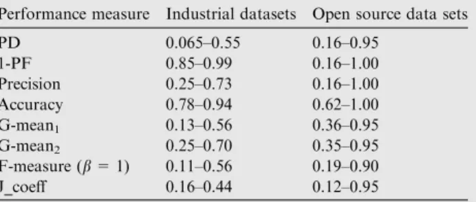
Performance indices have a following range in industrial and open source datasets as shown inTable 20.

It is rare that one model will be best for all the projects in software quality assessment. While some models will be advan-tageous when few modules are fault prone, others will show their prominence in traditional comparison methods for binary classiﬁcation like ROC or PR curves, thus providing easy adaptability in a wide range of project conditions.

We hope the approach and steps for evaluation given in this paper are capable to provide better understanding and hence would increase the statistical validity for future studies. References

Adams, N.M., Hand, D.J., 1999. Comparing classiﬁers when the misallocation costs are uncertain. Pattern Recognit. 32, 1139–1147. http://dx.doi.org/10.1016/S0031-3203(98)00154-X.

Aggarwal, K.K., Singh, Y., Kaur, A., Malhotra, R., 2006. Empirical study of object-oriented metrics. J. Object Technol. 5 (8), 149–173. Aggarwal, K.K., Singh, Y., Kaur, A., Malhotra, R., 2009. Empirical analysis for investigating the effect of object-oriented metrics on fault proneness: A replicated case study. Software Process Improv. Pract. 16 (1), 39–62.http://dx.doi.org/10.1002/spip.389s.

Basili, V., Briand, L., Melo, W.L., 1996. A validation of object-oriented design metrics as quality indicators. IEEE Trans. Software Eng. 22 (10), 751–761.

Bernstien, A., Ekanayake, J., Pinzger, M., 2007. In: Proceedings of IWPSE 2007 Ninth International Workshop on Principles of Software Evolution in Conjuction with the 6th_{ESEC/FSE Joint}

Meeting, pp. 11–18.http://dx.doi.org/10.1145/1294948.1294953. Boehm, B., Papaccio, P., 1988. Understanding and controlling

software costs. IEEE Trans. Software Eng. 14, 1462–1477. Briand, L., Wust, J., 2001. Replicated case studies for investigating

quality factors in object-oriented designs. Empir. Softw. Eng. 6 (1), 11–58.

Briand, L., Daly, J., Wust, J., 1999. A uniﬁed framework for coupling measurement in object-oriented systems. IEEE Trans. Software Eng. 25, 91–121.

Briand, L., Daly, J., Porter, V., Wust, J., 2000. Exploring the relationships between design measures and software quality. J. Syst. Software 5, 245–273.

Chidamber, S., Kemerer, C.F., 1994. A metrics suite for object-oriented design. In: IEEE Trans. Software Eng., vol. 6, pp. 476– 493, SE-20.

Conover, W.J., 1999. Practical Nonparametric Statistics. Wiley, New York.

Drummond, C., Holte, R.C., 2006. Cost curves: an improved method for visualizing classiﬁer performance. Mach. Learn. 65 (1), 95–130. http://dx.doi.org/10.1007/s10994-006-8199-5.

Demsar, J., 2006. Statistical comparisons of classiﬁers over multiple data sets. J. Mach. Learn. Res. 7, 1–30.

El Emam, K., Benlarbi, S., Goel, N., Rai, S., 2001a. The confounding effect of class size on the validity of object-oriented metrics. IEEE Trans. Software Eng. 27 (7), 630–650.

El Emam, K., Melo, W., Machado, J., 2001b. The prediction of faulty classes using object-oriented design metrics. J. Syst. Software 56, 63–75.

El Emam, K., Benlarbi, S., Goel, N., Rai, S., 2001c. Comparing case-based reasoning classiﬁers for predicting high-risk software com-ponents. J. Syst. Software 55 (3), 301–320.

Table 19 The ranks of classiﬁers to be used in Nemenyi test for Dr Java. Classiﬁer Rank Random Forest 6 Bagging 5 Naı¨ve Bayes 4.5 Logistic 3 J48 2 IB1 1

Table 20 Difference of ranges for performance indices in industrial and open source data sets.

Performance measure Industrial datasets Open source data sets

PD 0.065–0.55 0.16–0.95 1-PF 0.85–0.99 0.16–1.00 Precision 0.25–0.73 0.16–1.00 Accuracy 0.78–0.94 0.62–1.00 G-mean1 0.13–0.56 0.36–0.95 G-mean2 0.25–0.70 0.35–0.95 F-measure (b= 1) 0.11–0.56 0.19–0.90 J_coeﬀ 0.16–0.44 0.12–0.95

(15)

Fenton, N.E., Ohlsson, N., 2000. Quantitative analysis of faults and failures in a complex software system. IEEE Trans. Software Eng. 26 (8), 797–814.

Guo, L., Ma, Y., Cukic, B., Singh, H., 2004. Robust prediction of fault-proneness by random forests, Proc. 15th Int’l Symp. Software Reliability Eng..

Gyimothy, T., Ferenc, R., Siket, I., 2005. Empirical validation of object-oriented metrics on open source software for fault predic-tion. IEEE Trans. Software Eng. 31 (10), 897–910.

Henderson-Sellers, B., 1996. Object-Oriented Metrics, Measures of Complexity. Prentice Hall, ISBN 0-13-239872-9.

Hassan, A., Holt, R., 2005. The top ten list: dynamic fault prediction. In: 21st IEEE International Conference on Software Maintenance (ICSM’05), pp. 263–272, ISSN: 1063-6773.

Hassan, 2009. Predicting faults using the complexity of code changes. In: Proceedings of 31st International Conference on Software Engineering, ICSE 2009, pp. 78–88.

Jiang, Y., Cukic, B., Ma, Y., 2008. Techniques for evaluating fault prediction models. Empir. Software Eng. 13, 561–595.

Khoshgoftaar, T.M., Pandya, A.S., Lanning, D.L., 1995. Application of neural networks for predicting faults. Ann. Software Eng. 1 (1), 141–154.

Khoshgoftaar, T.M., Ganesan, K., Allen, E.B, Ross, F.D., 1997. Predicting fault prone modules with case based reasoning. In: Proceedings of the Eighth International Symposium on Software Reliability Engineering, pp. 27–35. http://dx.doi.org/10.1109/ ISSRE.1997.630845.

Khoshgoftaar, T.M., Ganesan, K., Allen, E.B., 2000. Case-based software quality prediction. Int. J. Software Eng. Knowl. Eng. 10 (2), 139–152.

Khoshgoftaar, T.M., Seliya, N., 2003. Analogy-based practical clas-siﬁcation rules for software quality estimation. Empir. Software Eng. 8 (4), 325–350.

Khoshgoftaar, T.M., Seliya, N., 2004. Comparative assessment of software quality classiﬁcation techniques: an empirical study. Empir. Software Eng. 9, 229–257.

Kim, S., Zimmermann, T., Whitehead, E., Zellar, A., 2007. Predicting faults from cached history. In: Proceedings of 29th International Conference on Software Engineering, pp. 489–498.http://dx.doi. org/10.1109/ICSE.2007.66.

Kubat, M., Holte, R.C., Matwin, S., 1998. Machine learning for the detection of oil spills in satellite radar images. Mach. Learn. 30 (2– 3), 195–215.http://dx.doi.org/10.1023/A:1007452223027.

Lewis, D., Gale, W., 1994. A sequential algorithm for training text classifiers. In: Annual ACM Conference on Research and Devel-opment in Information Retrieval, the 17th Annual International ACM SIGIR Conference on Research and Development in Information Retrieval. Springer-Verlag, New York, NY, pp. 3–12. Lessmann, S., Baesens, B., Mues, C., Pietsch, S., 2008. Benchmarking classification models for software defect prediction: a proposed framework and novel findings. IEEE Trans. Software Eng. 34 (4), 485–496.

Li, W., Henry, S., 1993. Object oriented metrics that predict maintainability. J. Syst. Software 23 (2), 111–122.

Ling, C.X., Li, C., 1998. Data mining for direct marketing: problems and solutions. In: Proc. of the 4th Intern. Conf. on Knowledge Discovery and Data Mining, pp. 73–79, New York.

Lorenz, M., Kidd, J., 1994. Object-Oriented Software Metrics. Prentice-Hall.

Malhotra, R., Jain, A., 2012. Fault prediction using statistical and machine learning methods for improving software quality. J. Inf. Process. Syst. 8 (2), 241–262.

Malhotra, R., 2014. Comparative analysis of statistical and machine learning methods for predicting faulty modules. Appl. Soft Comput. 21, 286–297.

Mahanti, R., Antony, J., 2005. Conﬂuence of six sigma, simulation and software development. Manag. Audit. J. 20 (7), 739–762.

McCabe & Associates, 1994. McCabe Object Oriented Tool User’s Instructions.

Menzies, T., DiStefano, J., Orrego, A., Chapman, R., 2004. Assessing Predictors of Software Defects, Proc. Workshop Predictive Soft-ware Models.

Menzies, T., Greenwald, J., Frank, A., 2007a. Data mining static code attributes to learn defect predictors. IEEE Trans. Software Eng. 33 (1), 2–13.http://dx.doi.org/10.1109/TSE.2007.256941.

Menzies, T., Dekhtyar, A., DiStefano, J., Greenwald, J., 2007b. Problems with precision: a response to comments on data mining static code attributes to learn defect predictors. IEEE Trans. Software Eng. 33 (9), 637–640.

Moser, R., Pedrycz, W., Succi, G., 2008. A comparative analysis of the efﬁciency of change metrics and static code attributes for defect prediction. In: ACM/IEEE 30th International Conference on Software Engineering, pp. 181–190, ISSN: 0270-5257.

Myrtveit, I., Stensrud, E., 1999. A controlled experiment to assess the beneﬁts of estimating with analogy and regression models. IEEE Trans. Software Eng. 25 (4), 510–525.

Myrtveit, I., Stensrud, E., Shepperd, M., 2005. Reliability and validity in comparative studies of software prediction models. IEEE Trans. Software Eng. 31 (5), 380–391.

Nagappan, N., Ball, T., 2005. Use of relative code churn measures to predict system defect density. In: Proceedings 27th International Conference on Software Engineering, 2005. ICSE 2005, pp. 284– 292, ISSN 0270-5257.

Nagappan, N., Ball, T., Murphy, B., 2006. Using Historical In-Process and Product Metrics for Early Estimation of Software Failures. ISSRE 6.

Ohlsson, N., Alberg, H., 1996. Predicting fault-prone software modules in telephone switches. IEEE Trans. Software Eng. 22 (12), 886–894.http://dx.doi.org/10.1109/32.553637.

Ohlsson, N., Eriksson, A.C., Helander, M.E., 1997. Early risk-management by identiﬁcation of fault-prone modules. Empir. Software Eng. 2 (2), 166–173. http://dx.doi.org/10.1023/ A:1009757419320.

Ostrand, T.J., Weyuker, E.J., Bell, R.M., 2005. Predicting the location and number of faults in large software systems. IEEE Trans. Software Eng. 31 (4), 340–355. http://dx.doi.org/10.1109/ TSE.2005.49.

Okutan, A., Yıldız, O.T., 2012. Software defect prediction using Bayesian networks. Empir. Software Eng. 19 (1), 154–181. Paulson, James W., Giancario, S., Eberlein, A., 2004. An empirical

study of open spource and closed source software products. IEEE Trans. Software Eng. 4 (4), 246–256.

Porter, A.A., Selby, R.W., 1990. Evaluating techniques for generating metric-based classiﬁcation trees. J. Syst. Software 12 (3), 209–218. Provost, F., Kohavi, R., 1998. Guest editors introduction: on applied

research in machine learning. Mach. Learn. 30 (2–3), 127–132. Pai, G., 2007. Empirical analysis of software fault content and fault

proneness using Bayesian methods. IEEE Trans. Software Eng. 33 (10), 675–686.http://dx.doi.org/10.1109/TSE.2007.70722. Siegel, S., 1956. Nonparametric Statistics. McGraw-Hill, New York. Selby, R.W., Porter, A.A., 1988. Learning from examples: generation

and evaluation of decision trees for software resource analysis. IEEE Trans. Software Eng. 14 (12), 1743–1756.

Schneidewind, N.F., 1992. Methodology for validating software metrics. IEEE Trans. Software Eng. 18 (5), 410–422.

Shepperd, M., Kadoda, G., 2001. Comparing software prediction techniques using simulation. IEEE Trans. Software Eng. 27 (11), 1014–1022.

Tang, M., Kao, M., Chen, M., 1999. An empirical study on Object-oriented metrics. In: Proceedings of Sixth International Software Metrics Symposium, pp. 242–249. http://dx.doi.org/10.1109/ METRIC.1999.809745.

Witten, I.H., Frank, E., 2005. Data mining: Practical Machine Learning Tools and Techniques. Morgan Kaufmann.

(16)

Yu, P., Systa, T., Muller, H., 2002. Predicting fault-proneness using OO metrics. An industrial case study. In: Proceedings of Sixth European Conference on Software maintenance and Reengineering, 99-107, ISSN, pp. 1534–5351.http://dx.doi.org/10.1109/CSMR.2002.995794. Yeresime, S., Lov, K., Rath, S.K., 2014. Statistical and Machine Learning for Software Fault Prediction Using CK Metric Suite: A Comparative Analysis, International Scholarly Research Notices (ISRN) Software Engineering Volume 2014, 15 pages, 2014. Article ID 251083.

Youden, W., 1950. Index for rating diagnostic tests. Cancer 3, 32–35. http://dx.doi.org/10.1002/1097-0142(1950)3:1<32:: AID-CNCR28 20030106>3.0.CO;2-3.

Yousef, W.A., Wagner, R.F., Loew, M.H., 2004. Comparison of non-parametric methods for assessing classiﬁer performance in terms of ROC parameters. In Proceedings of Applied Imagery Pattern Recognition Workshop, vol. 33, issue 13–15, pp. 190–195.