Nonparametric predictive inference for combined competing risks data

(1)

Durham Research Online

Deposited in DRO:

04 June 2014

Version of attached le:

Accepted Version

Peer-review status of attached le:

Peer-reviewed

Citation for published item:

Coolen-Maturi, T. and Coolen, F.P.A. (2014) 'Nonparametric predictive inference for combined competing risks data.', Reliability engineering system safety., 126 . pp. 87-97.

Further information on publisher's website:

http://dx.doi.org/10.1016/j.ress.2014.01.007

Publisher's copyright statement:

NOTICE: this is the author's version of a work that was accepted for publication in Reliability Engineering System Safety. Changes resulting from the publishing process, such as peer review, editing, corrections, structural formatting, and other quality control mechanisms may not be reected in this document. Changes may have been made to this work since it was submitted for publication. A denitive version was subsequently published in Reliability Engineering System Safety, 126, 2014, 10.1016/j.ress.2014.01.007.

Additional information:

Use policy

The full-text may be used and/or reproduced, and given to third parties in any format or medium, without prior permission or charge, for personal research or study, educational, or not-for-prot purposes provided that:

• a full bibliographic reference is made to the original source • alinkis made to the metadata record in DRO

• the full-text is not changed in any way

The full-text must not be sold in any format or medium without the formal permission of the copyright holders. Please consult thefull DRO policyfor further details.

Durham University Library, Stockton Road, Durham DH1 3LY, United Kingdom Tel : +44 (0)191 334 3042 | Fax : +44 (0)191 334 2971

(2)

Nonparametric Predictive Inference for Combined Competing

Risks Data

Tahani Coolen-Maturia,∗, Frank P.A. Coolenb

a_{Durham University Business School, Durham University, Durham, DH1 3LB, UK} b_{Department of Mathematical Sciences, Durham University, Durham, DH1 3LE, UK}

Abstract

The nonparametric predictive inference (NPI) approach for competing risks data has re-cently been presented, in particular addressing the question due to which of the competing risks the next unit will fail, and also considering the effects of unobserved, re-defined, un-known or removed competing risks. In this paper, we introduce how the NPI approach can be used to deal with situations where units are not all at risk from all competing risks. This may typically occur if one combines information from multiple samples, which can e.g. be related to further aspects of units that define the samples or groups to which the units belong or to different applications where the circumstances under which the units operate can vary. We study the effect of combining the additional information from these multiple samples, so effectively borrowing information on specific competing risks from other units, on the inferences. Such combination of information can be relevant to competing risks scenarios in a variety of application areas, including engineering and medical studies.

Keywords: Imprecise probability, lower and upper probability, nonparametric

predictive inference, competing risks, right-censored data, combined data.

1. Introduction

Nonparametric predictive inference (NPI) is a statistical method based on Hill’s as-sumption A(n) (Hill, 1968), which gives a direct conditional probability for a future

ob-servable random quantity, conditional on observed values of related random quantities (Augustin and Coolen, 2004; Coolen, 2006). A(n) does not assume anything else, and can

be interpreted as a post-data assumption related to exchangeability (De Finetti, 1974). Inferences based on A(n) are predictive and nonparametric, and can be considered

suit-able if there is hardly any knowledge about the random quantity of interest, other than the n observations, or if one does not want to use such information, e.g. to study effects of additional assumptions underlying other statistical methods. A(n) is not sufficient to

derive precise probabilities for many events of interest, but it provides bounds for prob-abilities via the ‘fundamental theorem of probability’ (De Finetti, 1974). These bounds

∗_{Corresponding author}

Email addresses: [email protected](Tahani Coolen-Maturi),

(3)

are lower and upper probabilities in imprecise probability theory (Augustin and Coolen, 2004; Walley, 1991; Weichselberger, 2001). A suitable, albeit informal, interpretation for lower and upper probabilities, is that a lower probability reflects the evidence in favour of the event of interest while an upper probability, or more accurately the difference between one and an upper probability, reflects the evidence against the event of interest. Short introductions to NPI, imprecise probability and its use in reliability have recently been presented (Coolen, 2011; Coolen et al., 2011; Coolen and Utkin, 2011).

In reliability and survival analysis, data on event times are often affected by right-censoring, where for a specific unit or individual it is only known that the event of interest has not yet taken place at a specific time. Coolen and Yan (2004) presented a general-ization of A(n), called rc-A(n), which is suitable for right-censored data. In comparison

to A(n), rc-A(n) uses the additional assumption that, at the moment of censoring, the

residual lifetime of a right-censored unit is exchangeable with the residual lifetimes of all other units that have not yet failed or been censored. The assumption rc-A(n) underlies

the inferences in this paper, for more details we refer to (Coolen and Yan, 2004; Yan, 2002).

Coolen et al. (2002) introduced NPI for some reliability applications, including lower and upper survival functions for the next future observation, illustrated with an applica-tion with competing risks data. They illustrated the lower and upper marginal survival functions, so each restricted to a single failure mode. Competing risks have been the topic of many research papers over recent decades. As examples of applications, Jiang (2010) applied a discrete competing risk model to bus motor failure data, Bunea et al. (2008) used competing risk methods to analyse military systems data, and Bocchetti et al. (2009) applied such methods for study of reliability of marine diesel engines. Sarhan et al. (2010) discussed and illustrated likelihood and classical statistical approaches to competing risks data, Coolen et al. (1992) presented a Bayesian competing risk approach to reliability for heat exchangers based on expert judgements. Maturi et al. (2010) presented NPI for competing risks data, in particular addressing the question due to which of the competing risks the next unit will fail. Related to this approach, Coolen-Maturi and Coolen (2011) considered the effects of unobserved, re-defined, unknown or removed competing risks. Recently, Coolen-Maturi (2014) introduced NPI to compare two groups under (observed or unobserved) competing risks.

In NPI for competing risks (Maturi et al., 2010), it is assumed that there areK failure modes and a unit fails due to the first occurrence of a failure mode, which is identified with certainty. We should point out that, in this paper, we will use the terms ‘failure mode’ and ‘competing risk’ interchangeably with the same meaning. Let Xn+1 denote

the failure time of a future unit, based on n observations, and let the corresponding notation for the failure time including indication of the actual failure mode k be Xk,n+1.

It is important to emphasize that Xk,n+1 is interpreted as the random failure time of a

future unit which is onlyat risk from failure modek. Different failure modes are assumed to occur independently. The competing risk data per failure mode consist of a number of observed times of failures caused by the specific failure mode considered, and right-censoring times caused by other failure modes or other reasons for right-right-censoring. Hence rc-A(n) can be applied per failure mode k for inference on Xk,n+1.

(4)

· · ·< xk,ik < c ik k,1 < c ik k,2 <· · ·< c ik k,s_k,ik < xk,ik+1 < c ik+1 k,1 < c ik+1 k,2 <· · ·< c ik+1 k,s_k,ik+1 < xk,ik+2 < . . . 6 6 6 6 6 6 6 6 6 tik k,0 t ik k,1 t ik k,2 . . . t . . . ik k,s_k,ik t ik+1 k,0 t ik+1 k,1 t ik+1 k,2 t ik+1 k,s_k,ik+1 t ik+2 k,0

Figure 1: NPI data representation, considering failure modek

xk,1 < xk,2 < . . . < xk,uk, and let n−uk be the number of the right-censored observations,

ck,1 < ck,2 < . . . < ck,n−uk, corresponding to failure mode k; these may be failure times due to other (independent) failure modes, or observations that are right-censored for other reasons, where it is assumed throughout that such censoring processes are independent of Xk,n+1. For notational convenience, let xk,0 = 0 and xk,uk+1 = ∞. Suppose further that there are sk,ik right-censored observations in the interval (xk,ik, xk,ik+1), denoted by

cik k,1 < c ik k,2 < . . . < c ik k,s_k,ik, so Puk

ik=0sk,ik = n−uk. It should be emphasized that we do not assume that each unit considered must actually fail, if a unit does not fail then there will be a right-censored observation recorded for this unit for each failure mode, as we assume that the unit will then be withdrawn from the study, or the study ends, at some point. The random quantity representing the failure time of the next unit, with all K

failure modes considered, is Xn+1 = min

1≤k≤KXk,n+1.

For ik = 0,1, . . . , uk, let tik,ik∗

k = c

ik

k,i∗

k (i.e. censoring time) for i

∗

k = 1,2, . . . , sk,ik and

tik

k,i∗

k = xk,ik (i.e. failure time or time 0) for i

∗

k = 0. For notational convenience, let

tik

k,s_k,ik+1 = t

ik+1

k,0 = xk,ik+1 for ik = 0,1, . . . , uk−1. Let ˜nck,r and ˜n_tik k,i∗

k

be the number of units in the risk set just prior to time ck,r and tik,ik∗_k, respectively, with the definition

˜

n0 = n + 1 for ease of notation. The risk set at a certain time contains all units that

have not failed or been right-censored before that time, and hence are indeed still at risk. Figure 1 represents the data and notation considering failure mode k.

The NPI lower and upper survival functions for the failure time of the next unit due to failure mode k, so if the unit were only at risk from this failure mode, are denoted by S_X

k,n+1(t) and SXk,n+1(t), respectively, and are as follows (Maturi et al., 2010; Coolen

et al., 2002). For t∈(tik

k,ak, t

ik

k,ak+1] withik = 0,1, . . . , uk and ak = 0,1, . . . , sk,ik,

S_X k,n+1(t) = 1 n+ 1 n˜tik_k,ak₊₁ Y {r:ck,r<tik_k,ak+1} ˜ nck,r + 1 ˜ nck,r (1)

and for t ∈[xk,ik, xk,ik+1) with ik = 0,1, . . . , uk,

SXk,n+1(t) = 1 n+ 1 n˜xk,ik Y {r:ck,r<x_k,ik} ˜ nck,r + 1 ˜ nck,r (2)

While predictive inference, as considered in this approach, is different to estimation, as it explicitly considers a single future unit instead of estimating characteristics of a population distribution, it is interesting to mention that these NPI lower and upper sur-vival functions bound the well-known Kaplan-Meier estimator (Kaplan and Meier, 1958), which is the nonparametric maximum likelihood estimator for the population survival

(5)

function in case of lifetime data with right-censored observations, for more details we refer to (Coolen and Yan, 2004; Coolen-Maturi et al., 2012).

If all the units are censored with regard to failure mode k (e.g. if all units failed due to other failure modes, where in this case ik =uk = 0), then the lower and upper survival

functions in (1) and (2) are equal to (Coolen-Maturi and Coolen, 2011)

S_X n+1(t) = ˜ n_tik k,ak+1 ˜ n_tik k,ak+1 + 1 and SXn+1(t) = 1 (3)

If the next unit considered is at risk from K independent failure modes, so with its failure time given by Xn+1 = min

1≤k≤KXk,n+1, then the NPI lower and upper survival

functions for its failure time are denoted by S_X

n+1(t) and SXn+1(t), respectively, and are

equal to S_X n+1(t) = K Y k=1 S_X k,n+1(t) and SXn+1(t) = K Y k=1 SXk,n+1(t) (4)

In Section 2 the main results of this paper are presented, considering combination of information from different groups for several scenarios. This is an important contribution to the literature on competing risks from the perspective of NPI, as in practice one may often have data from a variety of competing risks scenarios which are closely related in the sense that several competing risks occur in all scenarios but there is no full exchangeability (which would allow grouping of all data without further complications) due to some com-peting risks not applying in all scenarios. Such situations occur frequently in practice. In engineering contexts, the same systems may function in different locations under slightly different circumstances, with several failure modes occurring everywhere but some failure modes specific to one or a few locations. In medical contexts, some diseases may affect both males and females, while other diseases may be gender-specific. This paper presents a general theory of NPI for such circumstances. Section 3 presents an extensive example to illustrate the results, followed by some concluding remarks in Section 4.

2. NPI for Combined Competing Risks Data

We now present a generalization of the NPI approach to competing risks, by consid-ering the important situation of different groups of units, such that units from the same group are at risk from the same set of competing risks, but these sets differ for the differ-ent groups. Of course, it is typically assumed that there is at least some overlap between the sets of competing risks for different groups. In this case, the information in data from different groups about a specific failure mode, that applied to these groups, can be used to enhance inferences for a unit at risk from this failure mode. To enable such learning from information about other groups, we make the important assumption, throughout this paper, that a failure mode affects all units that are at risk from it in the same way, no matter which group the unit belongs to. And, as mentioned before but crucial to the approach, we assume throughout this paper that all failure modes that affect a unit do so independently. Section 2.1 introduces further notation and presents the main setting considered in this paper. This is followed by different scenarios. In Section 2.2 we consider

(6)

inference about a specific failure mode, using data from all groups of units that were at risk from this failure mode. Section 2.3 combines such inferences to NPI lower and upper survival functions for a future unit from a particular group, so taking all failure modes that affect such a unit into account. Section 2.4 also considers a future unit, but now without perfect knowledge of the group this unit belongs to. Finally, Section 2.5 briefly presents results for three other scenarios of possible interest.

2.1. Notation and setting

In addition to notation introduced above, suppose we have M groups to which in-dividual units can belong, denoted by G1, . . . , Gm, . . . , GM. The sets of failure modes

that affect units are different per group. In medical survival analysis, such groups can be defined, for example, by covariates indicating sex or aspects of lifestyle. In reliability analyses, one can think about units that are used in different production processes or at different sites. We suppose that we have failure time data from each group, with sample size nm >0 for group m ∈ {1, . . . , M}. We assume that in total there are K competing

risks, denoted by R1, . . . , RK. Let dmk be an indicator function defined as

dmk =

1 if units in group Gm can fail due to risk Rk

0 if not

We should emphasize that for dmk = 1 we may actually have observed failures in group

Gm due to risk Rk or this may not be the case; we assume in this paper that the values

dmk are known with certainty. With regard to the data, let

d∗_mk =

1 if at least one failure due to Rk has been observed for group Gm

0 if no failure due to Rk has been observed for group Gm

So dmk = 0 logically impliesd∗mk = 0, but if dmk = 1 the corresponding d∗mk can be either

1 or 0.

For an index set J ⊆ {1,2, . . . , K} we will be interested in the NPI lower and upper survival functions for units at risk from all failure modes Rk for k ∈ J (and no other

failure modes); these are denoted by S_J and SJ. Let Jm be such an index set referring to

the set of failure modes due to which units in group Gm can fail, so Jm ={k :dmk = 1}.

We further define the index set of observed risks in the data for group Gm byJm∗ ={k :

dmk = 1 andd∗mk = 1}.

Similarly, we define the index set of groups whose units can fail due to failure mode

Rk asIk={m:dmk = 1}, soIk ⊆ {1,2, . . . , M}. We will consider the information about

failure modeRkin the data sets for the groupsGm withm ∈Ik. Based on these combined

data, we consider inference on a future unit under the assumption that it is only at risk from failure modeRk; to emphasize that such an inference will be based on the data from

all groups Gm with m ∈ Ik, we will denote the NPI lower and upper survival functions

for such a future unit by S_I

k and SIk. This notation can again be extended to indicate if we only take information into account from groups for which this specific failure mode

Rk has actually been observed; we then denote the index set corresponding to the groups

for which this failure mode has been observed by I_k∗ = {m : dmk = 1 and d∗mk = 1},

with similar extension of the notation for the corresponding NPI lower and upper survival functions.

(7)

2.2. Failure mode Rk

It is interesting to consider inference about a failure modeRk, that is inference about

the failure time of a future unit which is only at risk from failure mode Rk. This is

of interest in its own right, to learn about this failure mode, but also for its use in the competing risks scenario for a future unit which is at risk from several failure modes, which will be presented in Section 2.3. We use all data from all the groups whose units could have failed due to this failure mode, so groups Gm with m ∈ Ik ={m : dmk = 1}.

With interest only in failures due to Rk, all failure times in the data for these groups

that were caused by other failure modes are considered as right-censored observations. Note that it is irrelevant here, due to the assumptions of independent failure modes, that units from different groups which are included in the data for this inference on Rk will

not all have been at risk from the same failure modes; it is of no relevance which specific other failure modes caused the failures at times which are treated here as right-censored observations. The lower and upper survival functions for a future unit which is only at risk from failure mode Rk, and based on all data from groups Gm with m ∈ Ik, are (as

mentioned in Section 2.1) denoted by S_I

k and SIk, these are straightforwardly derived from Equations (1) and (2), respectively, using all the data from groups Gm with m∈Ik

as explained here. This predictive inference is based on information fromPM

m=1(nm×dmk)

units in the data set.

If we consider only the observed failure modes, when interested in failures due to Rk,

we use the data from all groups in which at least one unit has failed due to this failure mode, so groups Gm with m ∈ Ik∗ = {m : dmk = 1 and d∗mk = 1}. The NPI lower and

upper survival functions for a future unit which is only at risk from failure mode Rk,

and based on data from groups Gm with m ∈ Ik∗, are denoted by SI_k∗ and SI∗

k; these are straightforwardly derived from Equations (1) and (2). This predictive inference is based on information from PM

m=1(nm×dmk×d

∗

mk) units in the data set.

2.3. Unit from a specific group

We now consider inference about the failure time of the next unit from a specific group

Gm, which can fail due to all failure modes that can affect units from this group, so failure

modes Rk with dmk = 1, hence with k∈Jm. The NPI lower and upper survival functions

for the failure time of this future unit from group Gm are given by

S_J_m(t) = Y k∈Jm S_I k(t) and SJm(t) = Y k∈Jm SIk(t) (5)

where S_I_k and SIk are as presented in Section 2.2. Hence, this inference combines, for each failure mode that is being considered, all the data from different groups as described in Section 2.2.

We can also consider inference about the next unit from groupGm but using only data

from groups for which the relevant failure modes actually have been observed. Then the NPI lower and upper survival functions are

S_J∗ m(t) = Y k∈J∗ m S_I∗ k(t) and SJ ∗ m(t) = Y k∈J∗ m SI∗ k(t) (6)

(8)

where S_I∗

k and SI

∗

k are as presented in Section 2.2.

This inference for the failure time of a future unit from group Gm, using combined

information from other groups for individual competing risks, is the main novel result presented in this paper. Such use of information from other groups is also known as ‘borrowing information’ from other groups in order to derive stronger inferences. Note that such borrowing of information from other groups is done separately for each relevant failure mode, and that the assumption that different risks affect the units independently is required to combine the NPI lower and upper survival functions for the different failure modes in this way.

2.4. Unit from an unspecified group

In the previous section, we derived the NPI lower and upper survival functions for the next unit from a specific group Gm, using data on specific competing risks from other

groups as well. Suppose now that we are interested in inference about a future unit from an unspecified group, so, at the time of the inference, we do not have the perfect information to which group the unit belongs. Out of the many possible scenarios for this situation, corresponding to different possible assumptions, we consider the following two. First, we will assume that we know that the unit belongs to a particular subset of the groups, say groups Gm with m ∈ I for index set I ⊆ {1, . . . , M}, and that the specific

group it belongs to can be inferred from the numbers of units observed in these groups thus far, based on an exchangeability assumption. Secondly, we will also assume that the unit belongs to a particular subset of the groups, but that no further assumptions are made and no further information is used.

For the first scenario, we start with the special case where we know that the next unit belongs to one of two groups from the groups Gm, m = 1, . . . , M, without loss of

generality say group G1 orG2, soI ={1,2}. We assume that the group this unit belongs

to can be inferred from the numbers of units in these two groups observed in the data thus far, so that its membership of either group is exchangeable with such memberships of previously observed units in these two groups. For example, in medical studies one may wish to make a prediction for the next patient without knowing, beforehand, the sex of this patient, and assume exchangeability with the sexes of the previous patients. The well-known Theorem of Total Probability can now be applied, with P(Gm) denoting the

probability that the next unit belongs to group Gm, and therefore P(G2) = 1−P(G1),

to derive the following lower and upper survival functions

S(t) =S_J₁(t)P(G1) +SJ2(t)P(G2) (7)

S(t) =SJ1(t)P(G1) +SJ2(t)P(G2) (8)

where S_J₁ and SJ1 (SJ2 and SJ2), as defined in Section 2.3, are the NPI lower and upper

survival functions given that the next unit is from group G1 (group G2) and considering the relevant risks per group, taking into account also the corresponding data per failure mode in other groups. We can use NPI for Bernoulli data (Coolen, 1998) for inference about P(G1) and P(G2), which gives NPI lower and upper probabilities which we present explicitly as bounds of intervals (both to limit further notation and to emphasize that

(9)

optimisation over these intervals takes place), as follows P(G1)∈ n1 N + 1, n1+ 1 N + 1 and P(G2)∈ n2 N + 1, n2+ 1 N + 1 where N =n1+n2

with the constraintP(G1)+P(G2) = 1. In order to derive the NPI lower survival function S(t) for this scenario, we must minimise the expression in Equation (7) for P(G1) in this

specified interval, doing so of course immediately leads to the corresponding optimal value for P(G2) in the related interval, through the constraint between these two probabilities.

We can do this optimisation point-wise, so for each value of t separately, in order to reflect the information available with regard to survival at specific times. Clearly, if

S_J

1(t) < SJ2(t) the minimum is achieved for P(G1) =

n1+1

N+1, while if SJ1(t) > SJ2(t) it

is achieved for P(G1) = _Nn₊₁1 (in case of equality the value of P(G1) is irrelevant). The

corresponding NPI upper survival functionS(t) is derived by similar maximisation, which is also straightforward to implement.

Still for this first scenario, we now consider the case that the next unit belongs to a known subset consisting of M ≥3 groups. The reasoning for this case is similar to that for two groups, but instead of NPI for Bernoulli data (Coolen, 1998) we now learn from the data about group membership using NPI for multinomial data Coolen and Augustin (2009). This is based on a different underlying latent variable representation than the NPI method for Bernoulli data; it could also be used for the case with two groups, but then it would lead to slightly larger imprecision and the assumed latent variable representation would probably be less reasonable for most practical situations (for more details on the underlying aspects of these two NPI approaches we refer to Coolen (1998); Coolen and Augustin (2009)). Applying, as before, the Theorem of Total Probability leads to

S(t) = X m∈I S_J_m(t)P(Gm) (9) S(t) = X m∈I SJm(t)P(Gm) (10)

where S_J_m and SJm are again as presented in Section 2.3. NPI for multinomial data (Coolen and Augustin, 2009) leads to lower and upper probabilities represented by the corresponding intervals for P(Gm),

P(Gm)∈ nm−1 N , nm+ 1 N subject to X m∈I P(Gm) = 1 where N = X m∈I nm

In order to obtain the NPI lower and upper survival functions, S(t) and S(t), we must solve two simple constraint optimisation problems. To derive the lower survival function

S(t) we need to minimise Equation (9) overP(Gm) with the constraints above. It is easily

seen that this is achieved by the following procedure. Let N =P

m∈Inm and letqI be the

number of groups I. If qI is even we assign the maximum possible value nm_N+1 toP(Gm)

for the groups Gm whose corresponding lower survival function valuesSJm(t) are theqI/2 smallest values of all these lower survival function values at t, and to the remainingqI/2

groups we assign the minimum value nm−1

(10)

principle, but the maximum possible value for P(Gm) is then assigned to the (qI−1)/2

groups with the smallest corresponding values of S_J_m(t), the minimum possible value for

P(Gm) is then assigned to the (qI−1)/2 groups with the largest corresponding values of

S_J_m(t), while the groupGm corresponding to the medium value ofSJm(t) will be assigned the probability nm

N . To derive the corresponding NPI upper survival function the same

reasoning leads to just the minima and maxima being interchanged, as the reader can easily verify.

The second scenario considered here is that we do not know to which group in a given subset of groups the next unit belongs, and we do not want to make a further exchangeability assumption with previously observed units in order to learn about the probability that it belongs to a specific group (as was done in the scenario above). In this case, the NPI lower and upper survival functions for this next unit are simply the envelopes of the NPI lower and upper survival functions of all the groups in the subset, so

S(t) = min

m∈I{SJm(t)} and S(t) = maxm∈I{SJm(t)}

where S_J_m and SJm are again as presented in Section 2.3.

2.5. Three other scenarios of possible interest

There are many more possible scenarios with regard to the information and assump-tions on competing risks that could be of practical interest. To illustrate this, we briefly consider three further scenarios. We do not illustrate these in the example in Section 3, but include them here to show that dealing with such variations is relatively straight-forward and follows similar steps as the main methods presented in this paper. First, suppose that we are not sure if units can fail due to failure modes which have not been observed for this group. Then the lower and upper survival functions for the next unit from group Gm are

S(t) = Y k∈Jm1 S_I_k(t) Y k∈Jm0 S_I_k(t) = S_J_m(t) and S(t) = Y k∈Jm1 SIk(t) =SJm1(t) (11)

where Jm1 = Jm∗ = {k : dmk = 1 and d∗mk = 1} and Jm0 = {k : dmk = 1 and d∗mk = 0}.

This lower survival function is based on the pessimistic assumption that the unit can indeed fail due to unobserved failure modes, while the upper survival function is based on the assumption that it can only fail due to observed failure modes.

Secondly, units from group Gm have failed due to one or more failure modes Rk∗

(k∗ ∈ {1, . . . , K}) in the past, but assume now that the units will not be at risk from these failure modes in the future, so these failure modes have been removed (Coolen-Maturi and Coolen, 2011). Then the lower and upper survival functions for the next unit from group Gm are

S(t) = Y k∈J∗ m1 S_I k(t) Y k∈Jm0 S_I k(t) and S(t) = Y k∈J∗ m1 SIk(t) Y k∈Jm0 SIk(t) (12)

where J_m∗₁ is defined as J_m∗₁ = Jm1\{k∗}, where Jm1 = {k : dmk = 1 and d∗mk = 1}.

These lower and upper survival functions follow straightforwardly due to the removal of the specific failure modes.

(11)

Thirdly, consider the situation where units from groupGm could not fail due to failure

modes Rk∗ (k∗ ∈ {1, . . . , K}) in the past, but these failure modes can cause such units

to fail in the future. Then the lower and upper survival functions for the next unit from group Gm are S(t) =S_J_m(t) Y k∗ S_I k∗(t) and S(t) = SJm(t) Y k∗ SIk∗(t) (13)

where S_J_m(t) and SJm(t) are obtained as in Section 2.3, and SIk∗ and SIk∗ are the lower and upper survival function for the next unit assuming that this can fail only due to failure mode Rk∗, which can be obtained using (1) and (2) presented in Section 2.2.

3. Example

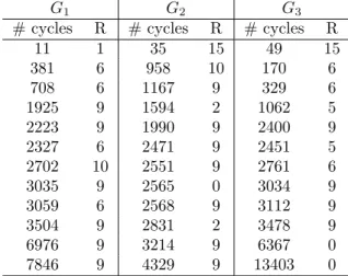
We illustrate the NPI methods presented in this paper via an extensive example based on a well-known data set from the literature (Lawless, 2003). The data contain information about 36 units of a new model of a small electrical appliance which were tested, and where the lifetime observation per unit consists of the number of completed cycles of use until the unit failed (we interpret this number as a continuous quantity). To illustrate our method, we have divided this data set into three groups, G1, G2 and G3, as presented

in Table 1, which also includes the specific failure mode (R) that caused the unit to fail. In the study, there were 18 different ways in which an appliance could fail, so 18 failure modes, but only 7 of them have been observed. Failure modesR9 and R6 caused 17 units

and 7 units to fail, respectively, while failure modes R2, R5, R10 and R15 each caused

two units to fail, and failure mode R1 caused one unit to fail. Three units in the test

did not fail before the end of the experiment, so for these units we have right-censored observations (2565, 6367 and 13403) for all failure modes considered, indicated by ‘0’ for the failure mode in Table 1. With this grouping of the data, there are 4 observed failure modes per group: failure modes R1, R6, R9 and R10 have been observed in group G1,

failure modes R2, R9, R10 and R15 have been observed in group G2, and failure modes R5, R6, R9 and R15 have been observed in groupG3.

G1 G2 G3

# cycles R # cycles R # cycles R

11 1 35 15 49 15 381 6 958 10 170 6 708 6 1167 9 329 6 1925 9 1594 2 1062 5 2223 9 1990 9 2400 9 2327 6 2471 9 2451 5 2702 10 2551 9 2761 6 3035 9 2565 0 3034 9 3059 6 2568 9 3112 9 3504 9 2831 2 3478 9 6976 9 3214 9 6367 0 7846 9 4329 9 13403 0

(12)

3.1. Failure mode Rk

We start by considering inference about a specific failure mode Rk, as described in

Section 2.2. We discuss the following two options. First, we assume that the units in all groups could have failed due to Rk, so we use the data for all groups. Secondly, we

assume that only units in groups in which Rk has actually been observed, were at risk

from Rk, so only data from such groups are included for the inferences. This inference is

in terms of the failure time of a future unit that is at risk fromRk only, and based on the

data according to the specific assumption under these two possible scenarios.

Figures 2-5 present the NPI lower and upper survival functions for the next unit which is at risk from Rk only, for k= 2,3,6,9, under the assumption that all units in the three

groups of the data set had been at risk from Rk, so based on all 36 observations. In these

figures we denote the NPI lower and upper survival functions byS_R

kandSRk,k= 2,3,6,9, respectively. Note that we only observed, in total, two failures due to failure mode R2,

and we did not observe any failure due to failure mode R3. This is reflected in Figures 2 and 3, respectively, as the NPI upper survival function only decreases at an observed failure time caused by the specific Rk, while the NPI lower survival function decreases

at every observation, so both at failure times and right-censoring times with regard to

Rk, the latter being failure times caused by other failure modes as well as actually

right-censored observations. The NPI upper survival functions remain quite large for Figures 2-4, of course particularly in Figure 3 where it remains at value 1. This reflects that these data provide little evidence (or none at all for R3) against the possibility that units may

actually not fail due to the failure mode that is being considered. The corresponding NPI lower survival function reflects the evidence in the data in favour of survival past time t, which decreases at every observation because the number of items in the data that were at risk at timet decreases. Beyond the largest observation, t= 13403, the NPI lower survival function is equal to zero, reflecting that the data do not contain evidence in favour of further survival.

We now consider the same inference, so failure time of a future unit which is assumed to be only at risk from failure modeRk, but we assume explicitly that this failure mode only

affected units in the groups in which it was actually observed. It should be emphasized that the decision on whether this is appropriate use of the data, or data from all groups can be used as presented above, is up to the topic expert and necessarily based on detailed information about the actual setting, clearly the data do not provide information to distinguish between these two scenarios or indeed between other possible scenarios, some of which are discussed in this paper and illustrated below. One may have an intermediate case where it was known that the failure mode did affect units in some groups where it was not observed, but not all such groups.

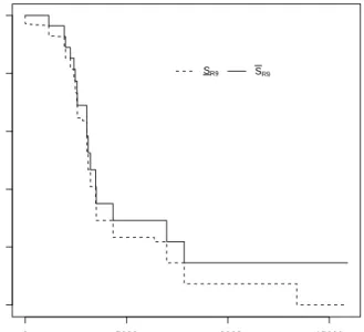
For the data in this example, separated in three groups as given in Table 1, the NPI lower and upper survival functions for some failure modes are presented in Figures 6-9, under the assumption that a specific failure mode only affected units in groups where it has actually been observed. This implies that inference for failure mode R9 is based on data from all the groups, as this failure mode was observed to cause failures in each group. Hence, the NPI lower and upper survival functions forR9 in this case, as presented

in Figure 8, are identical to those presented in Figure 5, because both cases take the observations from all groups into account. As another extreme situation, for any

(13)

non-0 5000 10000 15000 0.0 0.2 0.4 0.6 0.8 1.0 t Sur viv al function SR2 SR2

Figure 2: Lower and upper survival functions forR2(data: all groups)

0 5000 10000 15000 0.0 0.2 0.4 0.6 0.8 1.0 t Sur viv al function SR3 SR3

(14)

Figure 4: Lower and upper survival functions forR6(data: all groups)

(15)

Figure 6: Lower and upper survival functions forR2(data: only groups for whichR2has been observed)

(16)

Figure 8: Lower and upper survival functions forR9(data: only groups for whichR9has been observed)

(17)

observed failure mode there is now no meaningful inference, as no data are available to base inferences on. For example, using the data from all groups, we did get a non-trivial inference forR3, due to the fact that all items had functioned for some time without failing

due to this failure mode. But no such information is available under the assumption considered now. In the first situation, the information was reflected through the NPI lower survival function in Figure 3, which decreased at each right-censored observation. In this case with no data we can only provide the vacuous inference that the NPI lower survival function is equal to 0 and the NPI upper survival function is equal to 1 for all

t > 0. Note that this upper survival function is identical to the one for the situation above, which indeed reflects that there was no strong information in the data against the possibility failure mode R3 might never lead to failures.

Figures 6-9 also present the NPI lower and upper survival functions for failure mode

R2, using data from group G2 only, failure mode R6, using data from groups G1 and G3,

and failure mode R10, using data from groups G1 and G2. Of course, similar plots could

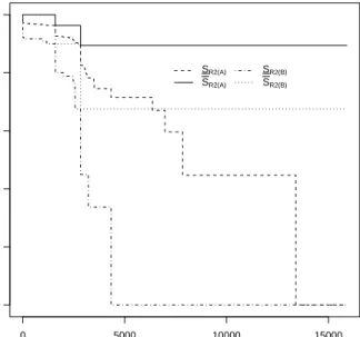
be presented for the NPI lower and upper survival functions for the other failure modes. It is interesting to compare the NPI lower and upper survival functions for R6 in Figure

4 and Figure 7, as these are based on different information. To emphasize the differences, these functions are presented together in Figure 10. The two NPI upper survival functions decrease only at the 7 observed failure times due toR6. However, using all data (indicated

by (A) in Figure 10) implies that more units did not fail due toR6, hence the data contain

less evidence against survival at any time t past the first time of a failure due toR6 than

for the situation where only data from groups G1 and G3 is used (indicated by (B) in

Figure 10). This is reflected by the fact that the NPI upper survival function for the first situation is greater than for the second situation, beyond the first failure time caused by

R6 (up to that time both are equal to 1). The NPI lower survival functions for R6 in

these two scenarios differ more, due to the fact that these functions decrease at every observation in the data set, so also at right-censored observations, and the use of the data from G2 in the first case discussed above (indicated by (A) in Figure 10) but not in the

second case (indicated by (B) in Figure 10) implies that with more data used the lower survival function decreases at more time points. The lower survival function when all data are used here is greater than the one based on data from G1 and G3 only, for all t up to the largest observation. This is because the additional information only consists of right-censoring times and hence provides some more information in favour of survival at any time until the largest observation, after which both these lower survival functions are equal to 0, reflecting that the data do not contain strong information in favour of surviving beyond the largest observation.

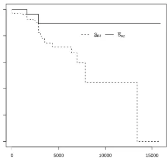
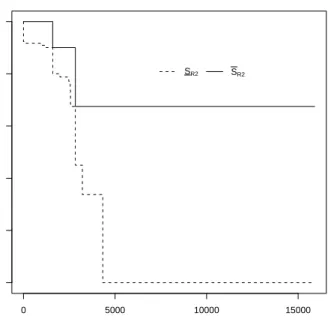
The same properties hold for the NPI lower and upper survival functions for failure mode R2 in Figure 2 and Figure 6, with the former based on the observations from all

groups, so from 36 units, but the latter only on the data from the 12 units in group G2.

These lower and upper survival functions are also presented together in Figure 11, to show the differences more clearly. In this latter case (indicated by (B) in Figure 11), the NPI lower survival function decreases only at 12 time points, the last one at t = 4329 from which moment on the lower survival function is equal to 0. With the largest observation in all combined data being at t = 13403, the lower survival function based on all combined data (indicated by (A) in Figure 11) only becomes 0 at that time point, so there is a

(18)

0 5000 10000 15000 0.0 0.2 0.4 0.6 0.8 1.0 t Sur viv al function SR6(A) SR6(A) SR6(B) SR6(B)

Figure 10: Lower and upper survival functions forR6: (A) using all data, (B) only data fromG1 andG3.

0 5000 10000 15000 0.0 0.2 0.4 0.6 0.8 1.0 t Sur viv al function SR2(A) SR2(A) SR2(B) SR2(B)

(19)

substantial difference between these two lower survival functions. While the two NPI upper survival functions for these cases both decrease only at the two observed failure times due to R2, the inclusion of many more right-censored observations (with regard to

this failure mode) in the first case leads to a substantial difference between these two upper survival functions.

3.2. Unit from a specific group

Next we illustrate the methods presented in Section 2.3, so we consider the failure time of the next unit from group Gm, where again assumptions are required about which

failure modes can affect this unit. There are several possible assumptions, we present those which we consider to be of most interest.

First, we assume that all failure modes that have been observed at least once affected the units from all three groups, so these are Rk for k = {1,2,5,6,9,10,15}. We are

interested in the failure time of a future unit which is at risk from precisely these 7 failure modes, so this could be a unit from any of the groups G1, G2 orG3. The NPI lower and

upper survival functions for such a future unit from any group, in this case, are presented in Figure 12, and they are derived by (for all m = 1,2,3)

S_J_m(t) = Y k∈{1,2,5,6,9,10,15} S_I k(t) and SJm(t) = Y k∈{1,2,5,6,9,10,15} SIk(t)

It should be emphasized that here we combine the NPI lower and upper survival functions for the individual failure modes that can affect the unit of interest, while we have used all available data to first derive these lower and upper survival functions along the lines as presented in Section 2.2 and illustrated earlier in this example. We could have added one or more of the identified but unobserved failure modes to this approach, if we wished to assume that these could indeed also affect such a future unit. Due to the NPI upper survival functions for such a failure mode being equal to 1 for all t, the upper survival function SJm would not be affected. However, the lower survival function SJm would be multiplied by the lower survival function(s) for such additional failure mode(s), which under the assumptions that they could have affected all data observations would (all) be equal to the lower survival function for R3 in Figure 3. This latter lower survival

function decreases at the same 36 time points asS_J_m, namely all observation times in the data, and hence the resulting lower survival function for the next unit would be less than the S_J_m given in Figure 12. This would show the effect of the unit being possibly affected by more failure modes (leading to the decrease of the lower survival function), but not necessarily so as these failure modes have not yet been observed so there is no strong evidence that they will actually have an effect (shown by the unchanged upper survival function).

Secondly, we assume that a future unit of groupGm is only affected by failure modes

already observed for that group. In addition, we assume that, for as far as the data are concerned, only units in groups for which a particular failure mode has been observed were actually affected by it and hence only data from these groups are used for the inference about a specific failure mode; this means using the NPI lower and upper survival functions shown in Figures 6-9 (and the corresponding ones for failure modes not shown in that figure). The resulting NPI lower and upper survival functions for units from groups G1,

(20)

0 5000 10000 15000 0.0 0.2 0.4 0.6 0.8 1.0 t Sur viv al function SJm SJm

Figure 12: Lower and upper survival functions forGm,m= 1,2,3, using all data

0 5000 10000 15000 0.0 0.2 0.4 0.6 0.8 1.0 t Sur viv al function SJ1* SJ1*

(21)

Figure 14: Lower and upper survival functions forG2, using data where failure modes are observed

(22)

G2 and G3 are presented in Figures 13, 14 and 15. The three upper survival functions

in this figure are quite similar, except the one for G2 does not decrease as quickly for

smaller values of t. The similarity is mostly due to failure modeR9, which is included for

each group and for which most failure observations were available. The early difference is mostly due to failure modeR6, which here affects units of groupsG1 andG3, but not units

of group G2, and this failure mode caused several early failures. The main similarities

and differences in these lower survival functions are due to the same effects. It is also interesting to consider when these three lower survival functions become equal to 0. For

G1, we have SJ∗

1(t) = 0 for t ≥ 7846, because at this point the lower survival function

for R1 becomes 0, as for this failure mode only the data from group G1 are used. For G2, SJ2∗(t) = 0 for t ≥ 4329, because at this point the lower survival function for R2

becomes 0, as for this failure mode only the data from group G2 are used. For G3, we

have S_J∗

3(t) = 0 for t ≥ 13403, because for this group the lower survival functions for

R5, R6, R9, R15 are used and these all only become 0 at this largest observation, as they

were all observed for group G3 so the data for this group are included.

It is also of interest to compare all NPI lower and upper survival functions in Figures 12- 15, as this shows the effect of the different assumptions made, both with regard to the failure modes that will affect the future unit of interest and with regard to the data used for each failure mode, which is based on the assumption about which failure modes affected the units in the data groups.

3.3. Unit from an unspecified group

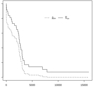
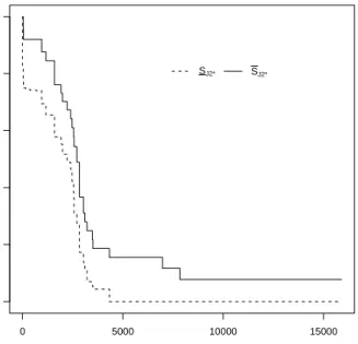
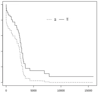
Finally, we briefly illustrate the NPI lower and upper survival functions for the main scenario presented in Section 2.4. Suppose we are interested in inference about the next unit, of which we only know that it belongs to a specified set of groups. We consider the three cases where we know that this unit belongs to one of two groups, and we only consider the observed competing risks per group only (so we assume that, per group, unobserved failure modes cannot affect the next unit). We make the assumption that we can learn about the membership of these groups from the data, where in this case each group had 12 observations. For example, if it is only known that the next unit belongs to group G1 orG3, then the lower and upper survival functions are

S(t) =S_J₁(t)P(G1) +SJ3(t)P(G3)

S(t) =SJ1(t)P(G1) +SJ3(t)P(G3)

where P(G1) ∈(12/25,13/25) and P(G3) = 1−P(G1). After optimization, these lower

and upper survival functions are given in Figures 16-18. These lower and upper survival functions are quite similar but of course still reflect some of the aspects of failure data in the individual groups as discussed before in this example.

4. Concluding remarks

This paper has presented the combination from different groups of data about shared failure modes, within the NPI framework of statistics. Such borrowing of strength by using data from other groups can be particularly important if there are only few observations,

(23)

0 5000 10000 15000 0.0 0.2 0.4 0.6 0.8 1.0 t Sur viv al function S S

Figure 16: Lower and upper survival functions for a future unit only known to belong toG1or G2

(24)

Figure 18: Lower and upper survival functions for a future unit only known to belong toG2or G3

or even none, for a specific failure mode in a group. It is important to emphasize that the decision on whether this is appropriate use of the data is up to the topic expert and is necessarily based on detailed information about the actual setting. The data themselves do not provide clear information about whether or not this is justified. The crucial assumptions are that failure modes affect units independently, and that a specific failure mode affects each unit that can be affected by it in the same manner. If one has a large number of data then these assumptions could be tested statistically, we do not consider this further in this paper as we mostly suggest this NPI method for small to medium size data sets. Indeed, for large data sets the NPI method effectively gives the empirical survival functions as imprecision becomes very small. Several main scenarios were presented, together with a few further ones that are also of practical interest. In the same way the method can be adapted to many further scenarios, following similar steps as presented for the main scenarios.

A clear challenge for research is to develop corresponding methods with weakening of the assumptions mentioned above. Theory of NPI for dependent data is being devel-oped and this may lead to opportunities for methods for dealing with dependent failure modes, but this would require data that go beyond the standard competing risk scenario considered in this paper, because if units are not used beyond their (first) failure then it is well known that the data do not contain information about dependence of the failure modes. One may also wish to link the methods presented in this paper with decision support, for example to consider optimal investment if one has a budget available to re-solve some failure modes. A further challenge is consideration of more than one future unit, whose failure times are not independent in the NPI approach. Whilst such NPI methods have been developed for real-valued data without right-censoring, and they are

(25)

quite straightforward to implement (Coolen, 2011), NPI for multiple future observations with right-censored data (as used in this paper) is a challenging topic for future research.

Acknowledgement

Tahani Coolen-Maturi thanks the Institute of Hazard Risk and Resilience at Durham University for financial support. We are grateful to three reviewers for suggestions that improved the presentation of this paper.

References

Augustin, T., Coolen, F. P. A., 2004. Nonparametric predictive inference and interval probability. Journal of Statistical Planning and Inference 124, 251–272.

Bocchetti, D., Giorgio, M., Guida, M., Pulcini, G., 2009. A competing risk model for the reliability of cylinder liners in marine diesel engines. Reliability Engineering & System Safety 94, 1299 – 1307.

Bunea, C., Mazzuchi, T. A., Sarkani, S., Chang, H.-C., 2008. Application of modern reli-ability database techniques to military system data. Relireli-ability Engineering & System Safety 93, 14 – 27.

Coolen, F., Mertens, P., Newby, M., 1992. A bayes-competing risk model for the use of expert judgment in reliability estimation. Reliability Engineering & System Safety 35, 23 – 30.

Coolen, F. P. A., 1998. Low structure imprecise predictive inference for bayes’ problem. Statistics & Probability Letters 36, 349–357.

Coolen, F. P. A., 2006. On nonparametric predictive inference and objective bayesianism. Journal of Logic, Language and Information 15, 21–47.

Coolen, F. P. A., 2011. Nonparametric predictive inference. In: Lovric, M. (Ed.), Inter-national Encyclopedia of Statistical Science. Springer, pp. 968–970.

Coolen, F. P. A., Augustin, T., 2009. A nonparametric predictive alternative to the im-precise dirichlet model: the case of a known number of categories. International Journal of Approximate Reasoning 50, 217–230.

Coolen, F. P. A., Coolen-Schrijner, P., Yan, K. J., 2002. Nonparametric predictive infer-ence in reliability. Reliability Engineering & System Safety 78, 185–193.

Coolen, F. P. A., Troffaes, M. C., Augustin, T., 2011. Imprecise probability. In: Lovric, M. (Ed.), International Encyclopedia of Statistical Science. Springer, pp. 645–648. Coolen, F. P. A., Utkin, L. V., 2011. Imprecise reliability. In: Lovric, M. (Ed.),

(26)

Coolen, F. P. A., Yan, K. J., 2004. Nonparametric predictive inference with right-censored data. Journal of Statistical Planning and Inference 126, 25–54.

Coolen-Maturi, T., 2014. Nonparametric predictive pairwise comparison with competing risks. Reliability Engineering & System Safety, Invited revision submitted.

Coolen-Maturi, T., Coolen, F. P. A., 2011. Unobserved, re-defined, unknown or removed failure modes in competing risks. Proceedings of the Institution of Mechanical Engi-neers, Part O: Journal of Risk and Reliability 225, 461–474.

Coolen-Maturi, T., Coolen-Schrijner, P., Coolen, F. P. A., 2012. Nonparametric predic-tive multiple comparisons of lifetime data. Communications in Statistics - Theory and Methods 41, 4164–4181.

De Finetti, B., 1974. Theory of Probability. Wiley, London.

Hill, B. M., 1968. Posterior distribution of percentiles: Bayes’ theorem for sampling from a population. Journal of the American Statistical Association 63, 677–691.

Jiang, R., 2010. Discrete competing risk model with application to modeling bus-motor failure data. Reliability Engineering & System Safety 95, 981 – 988.

Kaplan, E. L., Meier, P., 1958. Nonparametric estimation from incomplete observations. Journal of the American Statistical Association 53, 457–481.

Lawless, J. F., 2003. Statistical Models and Methods for Lifetime Data. Wiley, Hoboken, N.J.

Maturi, T. A., Coolen-Schrijner, P., Coolen, F. P. A., 2010. Nonparametric predictive inference for competing risks. Journal of Risk and Reliability 224, 11–26.

Sarhan, A. M., Hamilton, D. C., Smith, B., 2010. Statistical analysis of competing risks models. Reliability Engineering & System Safety 95, 953 – 962.

Walley, P., 1991. Statistical Reasoning with Imprecise Probabilities. Chapman & Hall, London.

Weichselberger, K., 2001. Elementare Grundbegriffe einer allgemeineren Wahrschein-lichkeitsrechnung I. Intervallwahrscheinlichkeit als umfassendes Konzept. Physika, Hei-delberg.

Yan, K. J., 2002. Nonparametric predictive inference with right-censored data. Ph.D. thesis, Durham University, Durham, UK, available from www.npi-statistics.com.