with Sparse Rule Bases. In: UKCI 16 - UK Workshop on Computational Intelligence, 7th -
9th September 2016, Lancaster, UK.
URL:
http://link.springer.com/chapter/10.1007%2F978-3-3...
<http://link.springer.com/chapter/10.1007%2F978-3-319-46562-3_8>
This version was downloaded from Northumbria Research Link:
http://nrl.northumbria.ac.uk/28259/
Northumbria University has developed Northumbria Research Link (NRL) to enable users to
access the University’s research output. Copyright
©and moral rights for items on NRL are
retained by the individual author(s) and/or other copyright owners. Single copies of full items
can be reproduced, displayed or performed, and given to third parties in any format or
medium for personal research or study, educational, or not-for-profit purposes without prior
permission or charge, provided the authors, title and full bibliographic details are given, as
well as a hyperlink and/or URL to the original metadata page. The content must not be
changed in any way. Full items must not be sold commercially in any format or medium
without formal permission of the copyright holder. The full policy is available online:
http://nrl.northumbria.ac.uk/policies.html
This document may differ from the final, published version of the research and has been
made available online in accordance with publisher policies. To read and/or cite from the
published version of the research, please visit the publisher’s website (a subscription may be
required.)
Jie Li, Yanpeng Qu, Hubert P. H. Shum, Longzhi Yang
AbstractThe Mamdani and TSK fuzzy models are fuzzy inference engines which have been most widely applied in real-world problems. Compared to the Mamdani approach, the TSK approach is more convenient when the crisp outputs are required. Common to both approaches, when a given observation does not overlap with any rule antecedent in the rule base (which usually termed as a sparse rule base), no rule can be fired, and thus no result can be generated. Fuzzy rule interpolation was proposed to address such issue. Although a number of important fuzzy rule interpo-lation approaches have been proposed in the literature, all of them were developed for Mamdani inference approach, which leads to the fuzzy outputs. This paper ex-tends the traditional TSK fuzzy inference approach to allow inferences on sparse TSK fuzzy rule bases with crisp outputs directly generated. This extension firstly calculates the similarity degrees between a given observation and every individual rule in the rule base, such that the similarity degrees between the observation and all rule antecedents are greater than 0 even when they do not overlap. Then the TSK fuzzy model is extended using the generated matching degrees to derive crisp infer-ence results. The experimentation shows the promising of the approach in enhancing the TSK inference engine when the knowledge represented in the rule base is not complete.
Jie Li, Hubert P. H. Shum, Longzhi Yang
Faculty of Engineering and Environment, Northumbria University, Newcastle upon Tyne, NE1 8ST, UK, e-mail:{jie2.li,hubert.shum,longzhi.yang}@northumbria.ac.uk
Yanpeng Qu
Information Science and Technology College, Dalian Maritime University, Dalian, 116026, China, e-mail:[email protected]
1 Introduction
Fuzzy inference system is a mechanism that uses fuzzy logic and fuzzy set theory to map inputs to outputs. Due to the simplicity and effectiveness in representing and reasoning on human natural language, it has become to one of the most ad-vanced technologies in control field. A typical fuzzy inference system consists of mainly two parts, a rule base (or knowledge base) and an inference engine. A num-ber of inference engines have been developed, with the Mamdani method [1] and the TSK method [2] being the most widely used. Mamdani fuzzy inference method is more intuitive and suitable for handling human natural language inputs, which is an implementation of the extension principle [3]. As fuzzy outputs are usually led by the Mamdani approach, a defuzzification approach, such as the centre of gravity method [4], has to be employed to map fuzzy outputs to crisp values for general system use. The TSK approach however uses polynomials to generate the inference consequence, and it therefore is able to directly produce crisp values as outputs, which is often more convenient to be employed when the crisp values are required. Both of these traditional fuzzy inference approaches require a dense rule base by which the entire input domain need to be fully covered; otherwise, no rule will be fired when a given observation does not overlap with any rule antecedent.
Fuzzy rule interpolation (FRI), firstly proposed in [5], not only addresses the above issue, but also helps in complexity reduction for complex fuzzy models. When a given observation does not overlap with any rule antecedent value, fuzzy rule interpolation is still able to obtain certain conclusion, and thus improves the applicability of fuzzy models. FRI can also be used to reduce the complexity of fuzzy models by removing those rules that can be approximated by their neighbour-ing ones. A number of fuzzy rule interpolation methods have been developed in the literature, including [6, 7, 8, 9, 10], and have been successfully employed to deal with real world application, such as [11, 12]. However, all of existing FRI methods were developed on (sparse) Mamdani rule bases which lead to fuzzy outputs.
This paper proposes a novel extension of traditional TSK fuzzy model, which is not only able to deal with sparse TSK fuzzy rule bases, but also able to directly gen-erate crisp outputs. To enable such extension, a new similarity degree measurement is proposed first to calculate the similarity degrees between given observations and each individual rule in the rule base. Dissimilar with the similarity measure used in the existing TSK approach, the introduced one leads to similarity degrees between the observation and others rule antecedents always greater than 0 even when they do not overlap at all. Then the TSK fuzzy model is extended using this new match-ing degree to obtain crisp inference results from sparse TSK fuzzy rule bases. The experiments show comparable result, which demonstrates the promising of the ap-proach in enhancing the traditional TSK model when the knowledge represented in the rule base is not complete.
The rest of the paper is structured as follows. Section 2 introduces the theoret-ical underpinnings of TSK fuzzy inference model and measurement of similarity degrees. Section 3 presents the proposed approach. Section 4 details a set of
exper-iments for comparison and validation. Section 5 concludes the paper and suggests probable future developments.
2 Background
In this section, the original TSK approach is briefly introduced, and the existing similarity measures are briefly reviewed.
2.1 TSK Fuzzy Model
The TSK fuzzy model was proposed by Takagi, Sugeno, and Kang in 1985 [2], and a typical fuzzy rule for the TSK model is of the following form:
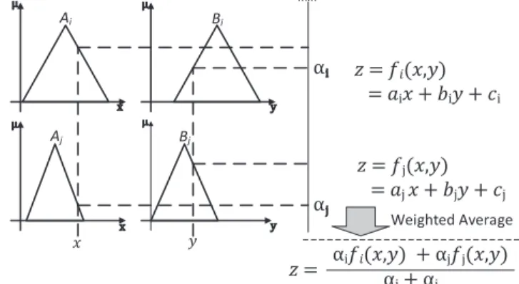
IFu is A and v is Bthenw✏f♣u, vq, (1) whereAandB are fuzzy sets regarding antecedent variablesxandyrespectively, andf♣u, vq is a crisp function (usually polynomial), which determines the crisp value of the consequent. For instance, assume that a rule base for TSK model is comprised of two rules:
Ri:IF x is Aiand y is BiTHENz✏fi♣x, yq ✏aix biy ci Rj:IF x is Ajand y is BjTHENz✏fj♣x, yq ✏ajx bjy cj,
(2) whereai,aj,bi,bj,ci, andcjare constants in the polynomial equation in the conse-quent part of the rule. The consequences of rulesRiandRjdeteriorate to constants ciandcj whenai ✏aj ✏ bi ✏bj ✏0. TSK model is usually employed to crisp inputs and outputs problems. Given an observation with singleton values as input (x0, y0), the working progress of this approach is demonstrated in Fig. 1. The in-ferred output from the given observation from rulesRi andRj arefi♣x0, y0qand fj♣x0, y0q respectively. The overall output is then taken as the weighted average of outputs from all rules, where the values of weights are the firing strengths of corresponding rules. Suppose thatµAi♣x0qandµBi♣y0qrepresent the matching
de-grees between input (x0, y0) and rulesRiandRj, respectively. The firing strength (weight) of ruleRi,αi, is calculated as:
αi✏µAi♣x0q ❫µBi♣y0q, (3)
where❫is a t-norm, which usually implemented as a minimum operator. Obviously, if a given input♣x1, y1qdoes not overlap with any rule antecedent, the matching degree between this input and rulesRi andRjareµAi♣x1qandµBi♣y1qare equal
to 0. Then no rule will be fired. Then, no consequence can be derived for such case. As the final result of the consequent variablezis a crisp value, the defuzzification
progress then can be saved, which in turn reduces the overall computational efforts. ρ ρ Ϥ ρ min Ƚ Ƚ ݖൌ݂݅ሺݔǡݕሻ ൌܽݔܾݕܿ ݖൌ݂ሺݔǡݕሻ ൌܽݔܾݕܿ ݖൌ Ƚ݂݅ሺݔǡݕሻȽ݂ሺݔǡݕሻ ȽȽ ݔ ݕ Weighted Average Ai Bi Aj Bj
Fig. 1 Representation of TSK approach
2.2 Similarity Degree Measurement
Based on different measurement standards, various similarity measures have been proposed in literature to calculate the degree of similarity between two fuzzy sets, such as[13, 14, 15, 16]. Note that, in order to generate reasonable mea-surement of similarity, the corresponding variable domain is required to be nor-malised first. Given two triangle fuzzy sets on the variable with nornor-malised domain, A ✏ ♣a1, a2, a3qandA✶ ✏ ♣a✶1, a✶2, a✶3q, where0 ↕ a1 ↕ a2 ↕ a3 ↕ 1, and 0↕a✶1↕a✶2↕a3✶ ↕1, the degree of similarityS♣A, A✶qbetween fuzzy setsAand A✶can be calculated as follows [13]:
S♣A, A✶q ✏1✁ 3 ➳ i✏1 ⑤ai✁a✶i⑤ 3 . (4)
The larger value ofS♣A, A✶qmeans that is the more similar between fuzzy setsA andA✶. This method is also the most wildly applied.
The above approach requires a normalisation progress for the concerned vari-able domain. A graded mean integration representation distance-based similarity degree measurement does not need such normalisation. This similarity measure is summarised as [17]:
S♣A, A✶q ✏ 1
1 d♣A, A✶q, (5)
whered♣A, A✶q ✏ ⑤P♣Aq ✁P♣A✶q⑤,P♣AqandP♣A✶qare the graded mean integra-tion representaintegra-tion ofAandA✶, respectively [17]. In particular, the graded mean integration representationP♣AqandP♣A✶qcan be defined as:
P♣Aq ✏ a1 4a2 a3 6 , P♣A✶q ✏ a ✶ 1 4a✶2 a✶3 6 . (6)
In this approach, the larger value of S♣A, A✶q means higher degree of similarity between fuzzy setsAandA✶.
The above two approaches may not provide correct similarity degrees in certain situations, such as two generalised fuzzy sets (which are fuzzy sets may not be normal), although they are usually able to produce acceptable results and widely applied. A generalised triangle fuzzy set regarding variablexcan be represented as A ✏ ♣a1, a2, a3, µ♣a2qq, where µ♣a2q (0 ➔ µ♣a2q ↕ 1) is the membership of elementa2, andµ♣a2q ➙ µ♣aq,❅a P Dx,Dxis the domain of variable x, as illustrated in Fig 2. Ifµ♣a2q ✏ 1, the generalised triangle fuzzy set deteriorates to normal a fuzzy set which is usually denoted as A ✏ ♣a1, a2, a3q. A centre of gravity method (COG) has been proposed to work with generalised fuzzy sets [15]. The process to calculate the COG-based similarity degree measure is summarised as below.
Step 1:Determine the point of centre of gravity for each triangle fuzzy set. Given a generalised triangle fuzzy setA, its COGG♣a✝, µ♣a✝qqis shown in Fig. 2, which can be calculated by:
a✝✏ a1 a2 a3
3 , (7)
µ♣a✝q ✏µ♣a1q µ♣a2q µ♣a3q
3 . (8)
Asµ♣a1q ✏µ♣a3q ✏0,µ♣a✝qcan be simplified to: µ♣a✝q ✏ µ♣a2q
3 . (9)
Step 2:Calculate the similarity degreeS♣A, A✶qbetween fuzzy setsAandA✶ by: S♣A, A✶q ✏ ✄ 1✁ 3 ➳ i✏1 ⑤ai✁a✶i⑤ 3 ☛ ☎ 1✁ ⑤a✝ A✁a✝A✶⑤ ✟B♣SuppA,SuppA✶q ☎min♣µ♣a✝Aq, µ♣a✝A✶q max♣µ♣a✝Aq, µ♣a✝A✶q , (10)
ሺʹǡρሺʹሻሻ 0 ݔ ρ ሺͳǡρሺͳሻሻ ሺ͵ǡρሺ͵ሻሻ COGሺȗǡρሺȗሻሻ ρሺʹሻ ρሺʹሻȀ͵ A
Fig. 2 A example triangular fuzzy set and its COG
wherea✝A anda✝A✶ are calculated by Equation 7,µ♣a✝Aqandµ♣a✝A✶q are obtained
from Equation 9, andB♣SuppA, SuppA✶qis defined as follow:
B♣SuppA, SuppA✶q ✏ ✩ ✫ ✪ 1, if SuppA SuppA✶ ✘0 0, if SuppA SuppA✶ ✏0, (11)
whereSuppAandSuppA✶are the supports of the fuzzy setsAandA✶respectively,
which in turn are calculated as:
SuppA✏a3✁a1, SuppA✶✏a✶3✁a✶1.
(12) In the above equation,B♣SuppA, SuppA✶qis used to determine whether COG dis-tance (1✁ ⑤a✝
A✁a✝A✶⑤) needs to be considered. For instance, if fuzzy setsAandA✶ both are the crisp values, (i.e.,SuppA ✏SuppA✶ ✏SuppA SuppA✶ ✏ 0), the COG distance will not be considered for the degree of similarity measure; other-wise, the COG distance will be considered. In this measure, again the larger value ofS♣A, A✶qmeans that the two fuzzy setsAandA✶are more similar.
3 The Proposed Approach
The proposed fuzzy rule interpolation approach regarding TSK style of inference is introduced in this section. In order to enable the extension, the existing measure of similarity degree between two fuzzy sets as shown in Equation 10 is modified first by introducing an extra monotone decreasing function of the geometric distances between the two fuzzy sets. Given an observation, the similarity degree between the given observation and each rule antecedent can then be calculated based on this modified similarity degree measure, which always results a similarity degree greater than 0 even when the two fuzzy sets are not overlapped. Then, a crisp inference re-sult can be obtained by considering all the rules associated with their corresponding matching degrees, based on underpinning principle of the original TSK inference.
As the similarity degrees between the given observation and all the rule antecedents are greater then 0, all the rules have firing strengths greater than 0, that is all rules are used for interpolation. Consequently, a crisp result can still be generated even when a given observation does not overlap with any rule antecedent.
3.1 A Modified Similarity Measure
The similarity measure expressed by Equation 10 may fail in certain situations, despite of its simplicity. For instance, if a large distance between two fuzzy sets presents, those two fuzzy sets should not similar at all. However, by applying this similarity measure, a big value of similarity degree, representing high similarity, may still be generated, which will lead to an unexpected result. In order to address this, the distance between fuzzy sets has been considered to extend this similarity measure [15]. However, the introduction of linear distance parameter may still not be sufficiently flexible to support various fuzzy models, as the sensitivity of sim-ilarity degree to distance is fixed. In order to provide a simsim-ilarity measure whose sensitivity to distance is flexible and configurable to support fuzzy interpolation for TSK model, the similarity measure introduced in [15] is extended. In particular, thedistance f actor(DF), which is an monotone decreasing function with an ad-justable parameter, is proposed to replace the linear distance function of the existing approach ([15]).
Suppose the variable domain has been normalised, and assume that there are two generalised triangle fuzzy setsA andA✶ regarding this variable, whereA ✏ ♣a1, a2, a3q, and A✶ ✏ ♣a✶1, a2, a✶ ✶3q. The degree of similarity S♣A, A✶q between fuzzy setsAandA✶can be calculated as follows:
S♣A, A✶q ✏ ✄ 1✁ 3 ➳ i✏1 ⑤ai✁a✶i⑤ 3 ☛ ☎ ♣DFqBr♣SuppA,SuppA✶q ☎min♣µ♣a✝Aq, µ♣a✝A✶qq max♣µ♣a✝Aq, µ♣a✝A✶qq , (13)
whereDF, termed asdistance f actor, is a function of the distance between the two concerned fuzzy sets.DF is in turn defined as:
DF ✏1✁ 1
1 e✁nd 5 , (14)
wheren(n → 0) is a sensitivity factor, anddrepresents the distance between the two fuzzy sets usually defined as the distance of their COGs. Smaller value of n leads to a similarity degree which is more sensitive to the distance of two fuzzy sets, and vice versa. The value of this factor needs to be determined based on the
specific problems. However, some early stage experimentation generally suggests that20↕n↕60. A further study of the automatic determination ofDF remains for the future work. It is worth to note that, there are two special situations where the modified similarity measure and Equation 10 lead to the same result: 1) when fuzzy setsAandA✶ have the same COG, and 2) whenAandA✶are two boundary crisp values and the distance between them is 1.
Compared to the approach proposed in [15], the modified similarity measure be-tween two given fuzzy sets preserves the same set of good properties, including 1) The lager value isS♣A, A✶q, the more similar are between fuzzy setsAandA✶, and 2) fuzzy setAandA✶ are identical if and only ifS♣A, A✶q ✏1. The proposed ap-proach also introduces one more important property, which is the similarity degree between any two fuzzy sets (excluding the two boundary crisp values that distance between them is 1) in the input domain will be always greater than 0. Without lose generality, given two fuzzy setsA ✏ ♣a1, a2, a3qandA✶ ✏ ♣a✶1, a✶2, a✶3qwithin a normalised input domain. Suppose that fuzzy setsA andA✶ are not the boundary sets, where0➔a1↕a2↕a3➔1, and0➔a✶1↕a✶2↕a✶3➔1. Then,
⑤a1✁a✶1⑤ ➔1, ⑤a2✁a✶2⑤ ➔1, ⑤a3✁a✶3⑤ ➔1.
(15)
This is followed by:
1✁ 3 ➳ i✏1 ⑤ai✁a✶i⑤ 3 → 0. (16)
Also,0➔DF ➔1based on Equation 14, andmin♣µ♣a✝
Aq, µ♣a✝A✶qq →0. According
to Equation 13, the value ofS♣A, A✶qmust be greater than 0.
3.2 Extending the TSK Model
For simplicity, this work only considers problems with two inputs and one output. A typical fuzzy rule for the original TSK fuzzy model is of the following form:
Ri: IFx is Aiand y is BiTHENz✏fi♣x, yq, (17) whereAi, andBiare fuzzy sets regarding input variablexandy, andfi♣x, yqis a crisp function which determines the consequence. For a given observation, the orig-inal TSK approach first determines those rules whose antecedents overlap with the given observation, and then obtains the firing strength (αi) of the overlapped rules by integrating the matching degrees between observation terms and rule antecedent terms. From this, the sub-consequence from each fired rule is computed using the consequent function. And finally, a crisp value of output (fi♣x, yq) is aggregated
by calculating the weighted average of the sub-consequences, as introduced in Sec-tion 2.1. If a given observaSec-tion does not overlap with any rule antecedent, no rule will be fired, and thus no inference can be made.
The above issue can be addressed by extending the original TSK approach using the similarity measure proposed in Section 3.1. Assume that a sparse rule base is comprised ofnrules, which is:
R1:IF x is A1and y is B1THENz✏f1♣x, yq ✏a1x b1y c1, ... ...
Ri:IF x is Aiand y is BiTHENz✏fi♣x, yq ✏aix biy ci, ... ...
Rn :IF x is Anand y is BnTHENz✏fn♣x, yq ✏anx bny cn, (18)
whereai,bi, andci(1↕i↕n) are constants of polynomials in rule consequences. When a inputO♣A✝, B✝q, alternatively termed as observation, is given, a crisp out-put can be generated by the following steps.
Step 1: Determine the matching degreesS♣A✝, Ai) andS♣B✝, Biqbetween the input values (A✝ andB✝) and rule antecedents (Ai andBi) for each rule using Equation 13.
Step 2: Calculate the firing degree of each rule by integrating the matching de-grees of its antecedents and the given inputs:
αi✏S♣A✝, Aiq ❫S♣B✝, Biq, (19) where❫is a t-norm, usually implemented by minimum operator in TSK inference model.
Step 3: Calculate the sub-consequence of the final result from each rule based on the given inputO♣A✝, B✝qand the polynomial in consequent.
fi♣A✝, B✝q ✏ai☎COG♣A✝q bi☎COG♣B✝q ci. (20) Step 4: Integrate the sub-consequences to get the final output:
z✏ n ➳ i✏1 αifi♣A✝, B✝q n ➳ i✏1 αi . (21)
As discussed earlier, the similarity degree between any two fuzzy sets (excludes the two boundary sets) in the input domain is always greater than 0. Therefore, different from traditional TSK method, which only considers those rules overlapped with the given observation, the proposed approach takes account all rules in the rule base to aggregate a crisp result. As a result, even if the given observation does not overlap with any rule antecedent in the rule base, certain inference result is still able
to be generated, which significantly improves the applicability of the original TSK approach.
4 Experimentation
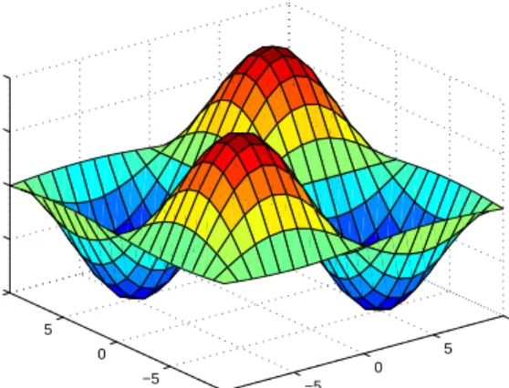
In order to validate and evaluate the proposed approach, a non-linear function, which has been considered in [18], is re-considered in this section to demonstrate the func-tionality of proposed system. The problem is to model the non-linear function given below: f♣x, yq ✏sin ✁x π ✠ sin ✁y π ✠ . (22)
The fuzzy model takes two inputs,x(xP r✁10,10s) andy(y P r10,10s), and produces a single outputz(z P r✁1,1s), as illustrated in Fig. 3. In order to enable the employment of the revised TSK style fuzzy rule interpolation, the input domains are normalised first. The normalisation maps any valuex0of variablextox✶0by:
x✶0✏
x0✁maxx
maxx✁minx , (23)
whereminxis the minimum value in the domain of variablex, andmaxx is the maximum value in the domain of variablex.
−10 −5 0 5 10 −10 −5 0 5 10 −1 −0.5 0 0.5 1 Input x Original Problem Model
Input y
Output z
Fig. 3 Surface view of the model
In order to generate a optimal sparse TSK rule base for the model, a dense rule base is generated first. Then some of the less important rules are removed manually to demonstrate the working of the proposed TSK style fuzzy rule interpolation
ap-proach. The evaluation of the proposed approach based on incomplete data remains as active work.
4.1 TSK Rule Base Generation
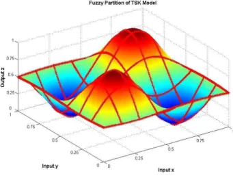
A dense TSK fuzzy rule base was generated based on the given model first, by which the entire input domain is fully covered. In order to do so, a training data set com-prised of 500 data points have been randomly generated from Equation 22. Then, a linear regression-based Matlab TSK rule base generation approach [19] was em-ployed to derive a normal TSK fuzzy rule base that partitions each antecedent vari-able domain by 7 fuzzy sets. The surface view of fuzzy partition of TSK model is also illustrated in Fig. 5. As there are two input variables, this leads to 49 fuzzy rules in total, as listed in Table 1 and shown in Fig. 4. Briefly, the employed data-driven approach first grid partitions the given input domain into sub-regions. Then, for each sub-region, a linear regression approach, the least-squares approach, is employed to represent the data in an initial fuzzy rule. After that, linear quadratic estimation (Kalman Filter) algorithm is used to fine tune the rules’ parameters until the satis-factory solution is found. The data-driven approach for TSK rule base generation is beyond the scope of this paper, and thus details are omitted here, however, more information can be found in [20].
0 x Ϥ 1 0.5 1 A1 A2 A3 A4 A5 A6 A7 0.167 0.333 0.667 0.833
(a) Normalised Inputx
0 y Ϥ 1 0.5 1 B1 B2 B3 B4 B5 B6 B7 0.167 0.333 0.667 0.833 (b) Normalised Inputy
Fig. 4 Fuzzy partition of domain of input
4.2 Sparse TSK Rule Base Generation
The TSK rule base was then simplified to sparse rule base, by which some obser-vations may not be covered by any rule antecedents in the rule base, to enable the evaluation of the proposed system. In this initial work, this progress was performed manually by removing some less important one, however, the study on sparse rule base generation or rule base simplification was left as future work. In particular, the size of the TSK rule base has been manually reduced 67%, which is comprised of
Fig. 5 Fuzzy partition for TSK modelling
Table 1 Generated TSK Rule Base
IF THEN IF THEN i x y z i x y z 1 A1 B1 0.315x 0.249y 0.501 26A4 B5 1.967x 0.164y✁0.472 2 A1 B2 1.589x 0.112y 0.494 27A4 B6 1.165x✁0.098y 0.087 3 A1 B3 1.366x✁0.075y 0.543 28A4 B7 ✁0.270x 0.220y 0.414 4 A1 B4 ✁0.296x✁0.139y 0.566 29A5 B1 0.064x✁1.463y 0.442 5 A1 B5 ✁1.181x✁0.058y 0.524 30A5 B2 ✁0.605x✁0.437y 0.526 6 A1 B6 ✁0.727x 0.373y 0.180 31A5 B3 ✁0.486 1.347y✁0.010 7 A1 B7 0.491x 0.551y✁0.033 32A5 B4 0.327x 2.060y✁0.629 8 A2 B1 0.188x 1.693y 0.485 33A5 B5 0.720x 0.930y✁0.116 9 A2 B2 0.568x 0.757y 0.710 34A5 B6 0.607x✁0.492y 0.841 10A2 B3 0.571x✁0.859y 1.052 35A5 B7 0.374x✁0.750y 0.802 11A2 B4 ✁0.044x✁1.379y 1.099 36A6 B1 0.283x✁1.098y 0.260 12A2 B5 ✁0.252x✁0.400y 0.337 37A6 B2 0.879x✁0.361y✁0.468 13A2 B6 ✁0.283x 0.630y✁0.305 38A6 B3 0.723x 0.840y✁0.634 14A2 B7 0.237x 0.595y 0.048 39A6 B4 0.066x 1.217y✁0.088 15A3 B1 0.020x 1.385y 0.508 40A6 B5 ✁0.832x 0.785y 1.012 16A3 B2 ✁1.100x 0.531y 1.136 41A6 B6 ✁0.115x✁0.073y 0.889 17A3 B3 ✁0.849x✁0.848y 1.373 42A6 B7 0.408x✁0.100y 0.127 18A3 B4 0.361x✁1.323y 0.956 43A7 B1 0.333x 0.342y 0.179 19A3 B5 1.409x✁0.460y✁0.049 44A7 B2 1.093x 0.063y✁0.404 20A3 B6 0.654x 0.663y✁0.529 45A7 B3 0.697x✁0.396y 0.102 21A3 B7 ✁0.375x 0.741y 0.037 46A7 B4 ✁0.308x 0.351y 0.554 22A4 B1 ✁0.009x✁0.280y 0.504 47A7 B5 ✁0.586x 0.322y 0.676 23A4 B2 ✁1.736x✁0.004y 1.262 48A7 B6 ✁0.021x 0.264y 0.163 24A4 B3 ✁1.341x 0.359y 0.958 49A7 B7 0.232x 0.112y 0.229 25A4 B4 0.502x 0.384y 0.084
23 rules:Ri, (i✏ t1,3,5,7,10,11,14,17,19,21,23,25,27,30,32,34,35,39,41, 43,45,47,49✉).
4.3 TSK Inference with Sparse Rule Base
To facilitate the comparison between the proposed approach and the approach pro-posed in [18], 36 testing data points were randomly generated by Equation 22 for testing and evaluation purpose. Note that although the considered problem in [18] was solved by Mamdani fuzzy model, it does not affect the result of the comparison as crisp results have been derived in this work using the defuzzification process.
To better illustrate the proposed approach, one randomly generated testing data pointO♣A✝ ✏0.299, B✝ ✏0.441qwas used as an example below to demonstrate the working progress of the proposed approach. Thedistance f actorin this exper-imentation is implemented as:
DF ✏1✁ 1
1 e✁20d 5 . (24)
From the given observation O♣0.299,0.441q, and the sparse rule base gen-erated in Section 4.2, the proposed approach first calculated the similarity de-gree between the given input and rule antecedents (S♣A✝, Aiq, S♣B✝, Biq) (i ✏ t1,3,5,7,10,11,14,17,19,21,23,25,27,30,32,34,35,39,41,43,45,47,49✉) us-ing Equation 13, with the results shown in the second and third columns of Table 2.
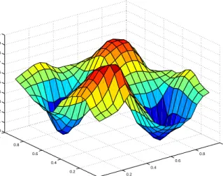
Based on the calculated similarity degree, the firing strength (FS) of each rule was calculated according to Equation 19, as shown in the fourth column of Table 2. From this, the sub consequence of the given observation from each rule was cal-culated by applying the observation to the linear function of rule consequence, as shown in the fifth column. The final result of variable (z) was then calculated by Equation 20, 21, which isz ✏ 0.566 in this demonstration. Note that the ground truth of the consequence for the given observation is 0.478, then the error is 0.088. Using the same approach, the errors for other 35 testing points were also calcu-lated. The reconstructed model based on the sparse TSK rule base with 23 rules (andDF ✏40) is demonstrated in Fig. 6 for comparison.
4.4 Result Analysis
By following the testing design and error representation of work [18], the sum of errors for the 36 randomly generated testing data points with different parameters have been summarised in Table 3. Also, to enable comparison, experiments based on sparse rule bases with 41,39,36,23 rules have also been conducted, with the
re-Table 2 The Calculation of Similarity Degree i S♣A✝, AiqS♣B✝, BiqF S♣A✝, B✝q Consequence 1 0.404 0.038 0.038 0.027 3 0.404 0.806 0.404 0.370 5 0.404 0.480 0.404 0.059 7 0.404 0.003 0.003 0.001 10 0.772 0.806 0.772 0.652 11 0.772 0.850 0.772 0.369 14 0.772 0.003 0.003 0.001 17 0.866 0.806 0.806 0.601 19 0.866 0.480 0.480 0.082 21 0.866 0.003 0.003 0.082 23 0.581 0.246 0.246 0.0008 25 0.581 0.850 0.581 0.205 27 0.581 0.033 0.033 0.013 30 0.055 0.276 0.055 0.008 32 0.055 0.850 0.055 0.021 34 0.055 0.033 0.055 0.027 35 0.055 0.003 0.055 0.002 39 0.002 0.850 0.002 0.0007 41 0.002 0.033 0.002 0.001 43 0.001 0.038 0.001 0.0005 45 0.001 0.806 0.001 0.0002 47 0.001 0.480 0.001 0.0008 49 0.001 0.003 0.001 0.0005
sults also shown in Table 3. From this table, it is clear that the proposed system outperforms the system proposed in [18].
The experimentation results suggest that sparser rule bases always lead to large errors, which is consistent with the intuitive expectation. It also can be seen from the result table that the sensitivity factor (n) indistance f actorindeed affects the accuracy of the inference results. Based on the initial investigation through this ex-perimentation, the system performs the best when the sensitivity factor is set to 40.
Table 3 Experimentation Results for Comparison
Numbers of Rules Proposed Approach Approach in [18] n=20n=40n=60 41 3.27 2.25 2.41 2.1 39 3.24 2.28 2.41 3.1 36 3.29 2.29 2.42 5.5 23 3.36 2.96 2.99 6.0
0 0.2 0.4 0.6 0.8 1 0 0.2 0.4 0.6 0.8 1 0 0.1 0.2 0.3 0.4 0.5 0.6 0.7 0.8 0.9 1 Input x Results with 23 Rules
Input y
Output z
Fig. 6 Surface view of results based on 23 rules
4.5 Discussion
Although many FRI approaches have been proposed to enable fuzzy inference with sparse rule bases, they were all developed on the Mamdani fuzzy model. The pro-posed approach is the first attempt to extend this idea to TSK fuzzy inference such that inference can be performed based on sparse rule bases. This will therefore pro-vide an additional alternative solution for those existing applications of FRI, such as [21] and in the same time to enjoy the advantages of TSK fuzzy inference. This will also enables extensions of existing FRI, such as the experience-based rule base generation and adaptation approach [21] to work with TSK inferences targeting a wider range of applications.
The rule base for traditional TSK fuzzy model, which used in this initial work, was generated by the linear regression algorithm, based on a randomly generated data set. Note that a recent development on sparse rule base updating and generat-ing has been reported[22]. Although this approach was implemented on the Mam-dani inference, the underpinning principle can be used to generate sparse TSK rule base. In particular, given a training data set, a sparse TSK rule base can be gen-erated directly from data by strategically locating the important regions for fuzzy modelling [22], thus to boost the applicability of the proposed approach.
5 Conclusion
This paper presented a novel approach to extend TSK inference to work with sparse rule bases. This is enabled by generating a crisp inference result based on all the rules in the rule base rather than only those whose antecedents overlap with obser-vations. In particular, the paper firstly proposed a new similarity degree measure by considering an extradistance f actorto obtain the similarity degree between the given observation and the corresponding rule antecedent of each rule. Then, based on the calculated degrees of similarity, all rules in the rule base will be considered with different firing strengths to generate a final crisp result. The experimentation shows that the proposed approach is not only able to deal with sparse TSK fuzzy rule bases, but is also able to generate competitive results in reference to the existing approach.
Although promising, the work can be further extended in the following areas. Firstly, the value of sensitivity factornindistance f actorwas arbitrarily given in this work based on some initial experimentation, and thus it would be worthwhile to further study how this parameter can be automatically determined or learned. Secondly, it is interesting to study if the curvature-based sparse rule base generation approach [22] can be used to support TSK rule base generation. Finally, it may be worthwhile, in further research, to investigate how the proposed approach can work with experience-based rule base generation [21].
References
1. E. H. Mamdani. Application of fuzzy logic to approximate reasoning using linguistic synthe-sis.Computers, IEEE Transactions on, C-26(12):1182–1191, 1977.
2. T. Takagi and M. Sugeno. Fuzzy identification of systems and its applications to modeling and control.Systems, Man and Cybernetics, IEEE Transactions on, SMC-15(1):116–132, 1985. 3. L.A. Zadeh. The concept of a linguistic variable and its application to approximate reasoning
- i.Information Sciences, 8(3):199 – 249, 1975.
4. Chuen Chien Lee. Fuzzy logic in control systems: fuzzy logic controller. ii. Systems, Man and Cybernetics, IEEE Transactions on, 20(2):419–435, 1990.
5. L. K´oczy and K. Hirota. Approximate reasoning by linear rule interpolation and general approximation.International Journal of Approximate Reasoning, 9(3):197–225, 1993. 6. Z. Huang and Q. Shen. Fuzzy interpolative reasoning via scale and move transformations.
Fuzzy Systems, IEEE Transactions on, 14(2):340–359, 2006.
7. Z. Huang and Q. Shen. Fuzzy interpolation and extrapolation: A practical approach. Fuzzy Systems, IEEE Transactions on, 16(1):13–28, 2008.
8. L.Yang and Q. Shen. Adaptive fuzzy interpolation and extrapolation with multiple-antecedent rules. InFuzzy Systems (FUZZ), 2010 IEEE International Conference on, pages 1–8, 2010. 9. L.Yang and Q. Shen. Adaptive fuzzy interpolation. Fuzzy Systems, IEEE Transactions on,
19(6):1107–1126, Dec 2011.
10. L.Yang and Q. Shen. Closed form fuzzy interpolation. Fuzzy Sets and Systems, 225:1 – 22, 2013. Theme: Fuzzy Systems.
11. J. Li, L. Yang, H. P. H. Shum, G. Sexton, and Y. Tan. Intelligent home heating controller using fuzzy rule interpolation. InUK Workshop on Computational Intelligence, 2015.
12. G.I. Molnarka, S. Kovacs, and L.T. K´oczy. Fuzzy rule interpolation based fuzzy signature structure in building condition evaluation. InFuzzy Systems (FUZZ-IEEE), 2014 IEEE Inter-national Conference on, pages 2214–2221, 2014.
13. S. M. Chen. New methods for subjective mental workload assessment and fuzzy risk analysis.
Cybernetics and Systems, 27(5):449–472, 1996.
14. B Sridevi and R Nadarajan. Fuzzy similarity measure for generalized fuzzy numbers. Int. J. Open Problems Compt. Math, 2(2):242–253, 2009.
15. S. J. Chen and S. M. Chen. Fuzzy risk analysis based on similarity measures of generalized fuzzy numbers.IEEE Transactions on Fuzzy Systems, 11(1):45–56, 2003.
16. L. Niyigena, P. Luukka, and M. Collan. Supplier evaluation with fuzzy similarity based fuzzy topsis with new fuzzy similarity measure. InComputational Intelligence and Informatics (CINTI), 2012 IEEE 13th International Symposium on, pages 237–244, 2012.
17. Shan Huo Chen and Chih Hsun Hsieh. Ranking generalized fuzzy number with graded mean integration representation. InProceedings of the Eighth International Conference of Fuzzy Sets and Systems Association World Congress, volume 2, pages 551–555, 1999.
18. H. Bellaaj, R. Ketata, and M. Chtourou. A new method for fuzzy rule base reduction.Journal of Intelligent & Fuzzy Systems, 25(3):605–613, 2013.
19. S. Konstantin. Sugeno-type FIS output tuning, 2010. http: //www.mathworks.com/matlabcentral/fileexchange/
28458-sugeno-type-fis-output-tuning.
20. Babak Rezaee and MH Fazel Zarandi. Data-driven fuzzy modeling for takagi–sugeno–kang fuzzy system.Information Sciences, 180(2):241–255, 2010.
21. J. Li, H. P. H. Shum, X. Fu, G. Sexton, and L. Yang. Experience-based rule base generation and adaptation for fuzzy interpolationn. InIEEE World Congress on Computation Intelligence Internation Conference, 2016.
22. Y. Tan, J. Li, M. Wonders, F. Chao, H. P. H. Shum, and L. Yang. Towards sparse rule base generation for fuzzy rule interpolation. InIEEE World Congress on Computation Intelligence Internation Conference, 2016.