Dissertations Theses and Dissertations
Spring 2014
Optimization of vehicle routing and scheduling
with travel time variability - application in winter
road maintenance
Haifeng Yu
New Jersey Institute of Technology
Follow this and additional works at:https://digitalcommons.njit.edu/dissertations
Part of theTransportation Engineering Commons
This Dissertation is brought to you for free and open access by the Theses and Dissertations at Digital Commons @ NJIT. It has been accepted for inclusion in Dissertations by an authorized administrator of Digital Commons @ NJIT. For more information, please contact
Recommended Citation
Yu, Haifeng, "Optimization of vehicle routing and scheduling with travel time variability - application in winter road maintenance" (2014).Dissertations. 181.
The copyright law of the United States (Title 17, United
States Code) governs the making of photocopies or other
reproductions of copyrighted material.
Under certain conditions specified in the law, libraries and
archives are authorized to furnish a photocopy or other
reproduction. One of these specified conditions is that the
photocopy or reproduction is not to be “used for any
purpose other than private study, scholarship, or research.”
If a, user makes a request for, or later uses, a photocopy or
reproduction for purposes in excess of “fair use” that user
may be liable for copyright infringement,
This institution reserves the right to refuse to accept a
copying order if, in its judgment, fulfillment of the order
would involve violation of copyright law.
Please Note: The author retains the copyright while the
New Jersey Institute of Technology reserves the right to
distribute this thesis or dissertation
Printing note: If you do not wish to print this page, then select
“Pages from: first page # to: last page #” on the print dialog screen
The Van Houten library has removed some of the
personal information and all signatures from the
approval page and biographical sketches of theses
and dissertations in order to protect the identity of
NJIT graduates and faculty.
MAINTENANCE by
Haifeng Yu
This study developed a mathematical model for optimizing vehicle routing and scheduling, which can be used to collect travel time information, and also to perform winter road maintenance operations (e.g., salting, plowing). The objective of this research was to minimize the total vehicle travel time to complete a given set of service tasks, subject to resource constraints (e.g., truck capacity, fleet size) and operational constraints (e.g., service time windows, service time limit).
The nature of the problem is to design vehicle routes and schedules to perform the required service on predetermined road segments, which can be interpreted as an arc routing problem (ARP). By using a network transformation technique, an ARP can be transformed into a well-studied node routing problem (NRP). A set-partitioning (SP) approach was introduced to formulate the problem into an integer programming problem (IPP). To solve this problem, firstly, a number of feasible routes were generated, subject to resources and operational constraints. A genetic algorithm based heuristic was developed to improve the efficiency of generating feasible routes. Secondly, the corresponding travel time of each route was computed. Finally, the feasible routes were entered into the linear programming solver (CPLEX) to obtain final optimized results. The impact of travel time variability on vehicle routing and scheduling for transportation planning was also considered in this study. Usually in the concern of vehicle and pedestrian’s safety, federal, state governments and local agencies are more
ii
would rather have a redundancy of plow trucks than a shortage. The proposed model and solution algorithm were validated with an empirical case study of 41 snow sections in the northwest area of New Jersey. Comprehensive analysis based on a deterministic travel time setting and a time-dependent travel time setting were both performed. The results show that a model that includes time dependent travel time produces better results than travel time being underestimated and being overestimated in transportation planning In addition, a scenario-based analysis suggests that the current NJDOT operation based on given snow sector design, service routes and fleet size can be improved by the proposed model that considers time dependent travel time and the geometry of the road network to optimize vehicle routing and scheduling. In general, the benefit of better routing and scheduling design for snow plowing could be reflected in smaller minimum required fleet size and shorter total vehicle travel time. The depot location and number of service routes also have an impact on the final optimized results. This suggests that managers should consider the depot location, vehicle fleet sizing and the routing design problem simultaneously at the planning stage to minimize the total cost for snow plowing operations.
by Haifeng Yu
A Dissertation Submitted to the Faculty of New Jersey Institute of Technology
in Partial Fulfillment of the Requirements for the Degree of Doctor of Philosophy in Transportation
Department of Civil and Environmental Engineering
Copyright © 2014 by Haifeng Yu ALL RIGHTS RESERVED .
MAINTENANCE Haifeng Yu
Dr. Steven I-Jy Chien, Dissertation Advisor Date Professor of John A. Reif, Jr. Department of Civil Environmental Engineering, NJIT
Dr. Lazar N. Spasovic, Committee Member Date
Professor of John A. Reif, Jr. Department of Civil Environmental Engineering, NJIT
Dr. Athanassios K. Bladikas, Committee Member Date
Associate Professor of Department of Mechanical and Industrial Engineering, NJIT
Dr. Janice R. Daniel, Committee Member Date
Associate Professor of John A. Reif, Jr. Department of Civil Environmental Engineering, NJIT
Dr. Jian Yang, Committee Member Date
Degree:
Doctor of Philosophy
Date:
May 2014
Undergraduate and Graduate Education:
•
Doctor of Philosophy in Transportation Engineering,
New Jersey Institute of Technology, Newark, NJ, 2014
Master of Science in Manufacturing System Engineering,
New Jersey Institute of Technology, Newark, NJ, 2009
•
Bachelor of Science in Electrical Engineering,
Guangdong University of Technology, Guangzhou, P. R. China, 2006
Major:
Transportation Engineering
Presentations and Publications:
Yu, Haifeng, Steven I-Jy Chien, and Ching-
Jung Ting. “Bilevel Programming Model forMinimum-Cost Travel Time Dat
a Collection with Time Windows.”Transportation Research Record: Journal of the Transportation Research Board
2197.-1 (2010): 29-35.
Yu, Haifeng, Steven I-Jy Chien, and Ching-
Jung Ting. “Optimal Routing for MinimumService Time of Winter Road Maintenance with Truck Capacity and Fleet Size
Constraints.” Transportation Research Board Annual Meeting, 2013, WashingtonDC.
A bdel - Malek, L ayek L., Steven I. Chien, Jay N. Meegoda, and H aifeng Y u
. “A Fleet Contracting Model for Snow Plowing Operations.” Journal of InfrastructureSystem, American Society of Civil Engineering, 2014
•
v
This dissertation is dedicated to my beloved family: my mother, Manhong Xiao;
my father, Guoqiang Yu; my girl friend, Chiewsze Cheah;
vi
ACKNOWLEDGMENT
I owe a great debt of gratitude to my advisor, Dr. Steven (I-Jy) Chien, who made this dissertation possible. He made outstanding contributions to my research by spending tons of time and effort turning my manuscript drafts into a high quality dissertation. During my five-year graduate study at NJIT, I had the privilege of having him as my instructor and mentor, and learned from him to be an independent thinker and excellent problem solver.
A special note of thanks goes to Dr. Athanassios K.Bladikas, Dr. Janice R. Daniel, Dr. Lazar N. Spasovic and Dr. Jian Yang in my Committee for their teaching, assistance, comments and suggestions.
Finally, I want to express my deep appreciation for the support and encouragement of my girlfriend, Chiewsze Cheah. Without her support and patience, this dissertation would not have been possible. I am also profoundly grateful to my parents for having faith on me and always encouraging me to challenge myself to move forward.
vii
Chapter Page
1 INTRODUCTION ………..………..….. 1
1.1 Background ………...……….……….…... 1
1.2 The Nature of the Problem ……….……….… 2
1.3 Objective and Work Scope ……….. 4
1.4 Dissertation Organization ……… 5
2 LITERATURE REVIEW ……….……….…. 7
2.1 Variability of Travel Time (VTT) …………...………..… 7
2.1.1 Impacts of VTT on Routing and Scheduling ……..……….. 9
2.1.2 Technologies for Collecting Travel Time Data ………. 12
2.2 Node Routing Problem …...………..…... 15
2.2.1 Vehicle Routing Problem with Pickup and Delivery (VRPPD) ……… 15
2.2.2 Vehicle Routing Problem with Time Windows (VRPTW) ………….. 16
2.2.3 Vehicle Routing Problem with Time-dependent Travel Time ……….. 18
2.3 Arc Routing Problem .……….……….……… 22
2.4 Transformation between NRP and ARP ……….. 24
viii (Continued)
Chapter Page
2.4.2 Transformation of ARP to NRP ……….…..….… 25
2.5 Vehicle Routing in Winter Road Maintenance ………....…… 26
2.5.1 Vehicle Routing Problems for Spreading ………..…..….. 27
2.5.2 Vehicle Routing Problems for Snow Plowing ……….…….. 29
2.6 Solution Algorithms ………. 32 2.6.1 Exact Algorithms ……….…..… 32 2.6.2 Heuristic Algorithms ……….…… 37 2.7 Summary ………..………….... 42 3 MODEL DEVELOPMENT ……… 44 3.1 Problem Description ………...……….……… 47 3.2 Network Transformation ………...……… 48
3.3 The Basic Model ………. 50
3.3.1 Assumptions ………...….. 51
3.3.2 Model Formulation ……… 51
3.4 The Enhanced Model ………...………. 53
ix (Continued)
Chapter Page
3.4.2 Time-Dependent Travel Time ………... 54
3.5 Set Partitioning Formulation ……….….. 56
3.6 Summary ……….…. 58
4 SOLUTION ALGORITHM ……….…….. 60
4.1 Exhaustive Numeration ……….……….…... 60
4.2 The Genetic Algorithm Based Heuristic .……….……….…….. 62
4.3 Summary ……….. 68
5 MODEL TESTING AND EVALUATION ……….………... 70
5.1 Example I-Travel Time Data Collection...………..………. 70
5.1.1 Numerical Results ………. 72
5.1.2 Scenario Analysis ……….. 77
5.1.3 Sensitivity Analysis ……… 78
5.2 Example II- Winter Road Maintenance …….……….…….… 82
5.2.1 Numerical Results ……….………..……... 84
5.2.2 Scenario Analysis ……….. 90
x (Continued)
Chapter Page
6 CASE STUDY ………..……….. 93
6.1 Objective ……….……….………... 93
6.2 Current Winter Roadway Maintenance in New Jersey ……….……….. 94
6.3 Data Preparation ……….. 96 6.3.1 Geometric Data ……….. 98 6.3.2 Weather Data ………. 100 6.3.3 Speed Data ………. 100 6.4 Results Discussion ………... 102 6.4.1 Scenario Analysis ………... 103
6.4.2 Sensitivity Analysis on Plowing Speed ………. 113
6.5 Summary ……….. 115
7 COMPUTATIONAL ANALYSIS ……….……….……….…….. 117
7.1 Optimal Results and Calulation Time ……….………… 117
7.2 Analysis on Population Size ……… 120
8 CONCLUSIONS AND FUTURE WORK ………. 122
xi (Continued)
Chapter Page
8.2 Future Work ……….……… 124
xii
Table Page
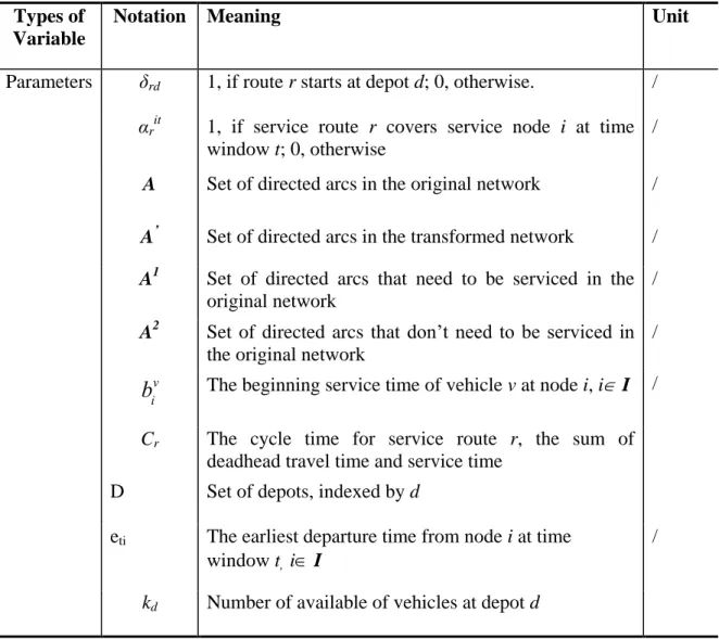
3.1 Glossary of Mathematical Notations (Alphabetical Order) ………... 46
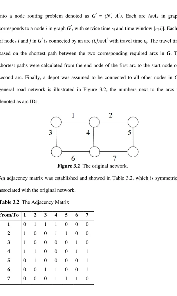
3.2 The Adjacency Matrix ………... 49
4.1 Sample of Chromosome Representation ……… 64
5.1 Characteristics of the Study Road Segments ………. 71
5.2 Travel Time and Distance Between Nodes ……… 72
5.3 Cost of Travel between Nodes (Unit: $) ……… 73
5.4 Node Assignment Travel Time/Cost Matrix for Time Window T2 ………... 74
5.5 Vehicle Availability Matrix for T2 ………. 74
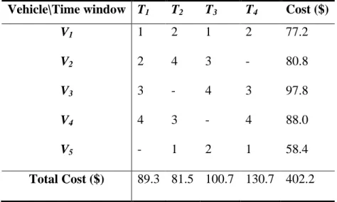
5.6 Feasible Routes and Schedules for Vehicles (Fleet Size = 5) ……… 75
5.7 Optimal Vehicle Schedule/Route Arrangement and the Minimized Cost ………. 76
5.8 Characteristics of Scenario A and B ……….. 77
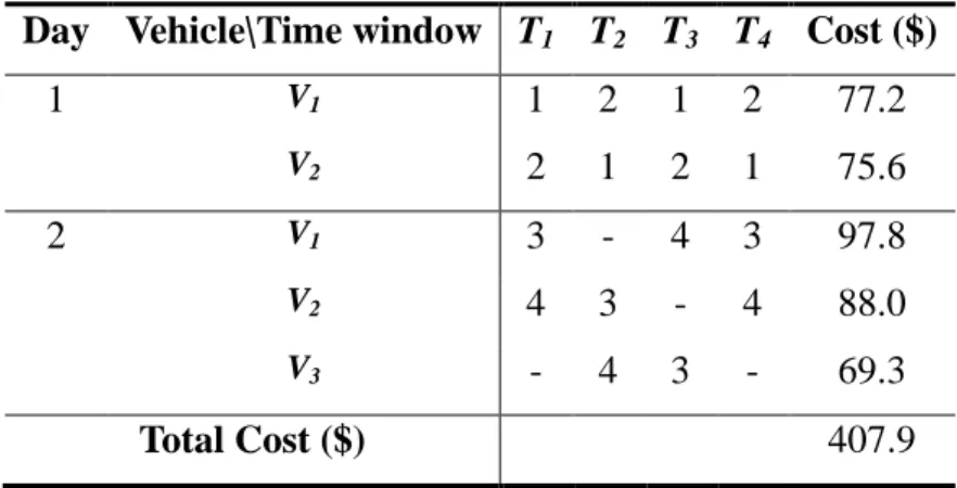
5.9 Optimal Vehicle Schedule and Minimized Cost (Fleet Size: 3) ……… 78
5.10 List of Required Arcs and Unrequired Arcs ……….. 85
5.11 Travel Distances Matrix ………. 86
5.12 Parameters and Notations (Alphabetical Order) ……….... 87
5.13 Results of Scenario I and Scenario II ………. 90
5.14 Results of Scenario III ………... 91
6.1 Expenditures in New Jersey for Winter Roadway Maintenance ………... 96
6.2 Selected Snow Sections and Maintenance Yards ……….. 98
xiii (Continued)
Table Page
6.4 Speed Profile of Road Type III at Different Time Period of PM peak ………….. 102
6.5 Definitions of Common Terms ……….. 103
6.6 Definitions of Scenarios ………..….. 104
6.7 Summary of Service Routes in Sussex ……….. 107
6.8 Summary of Results for Scenario-I ……… 108
6.9 Summary of Results for Scenario-II ……… 110
6.10 Results and Analyses for Various Plow Speed ……….. 114
7.1 Parameters of the GA Based Heuristic ……….. 118
7.2 Result comparison of Small Size Problems ………... 118
xiv
Table Page
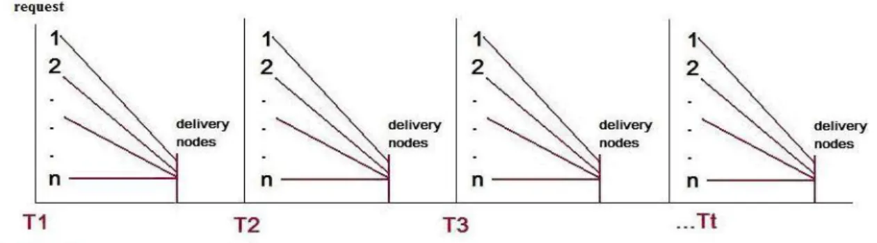
1.1 "Requests" at multiple time windows ………..……….. 3
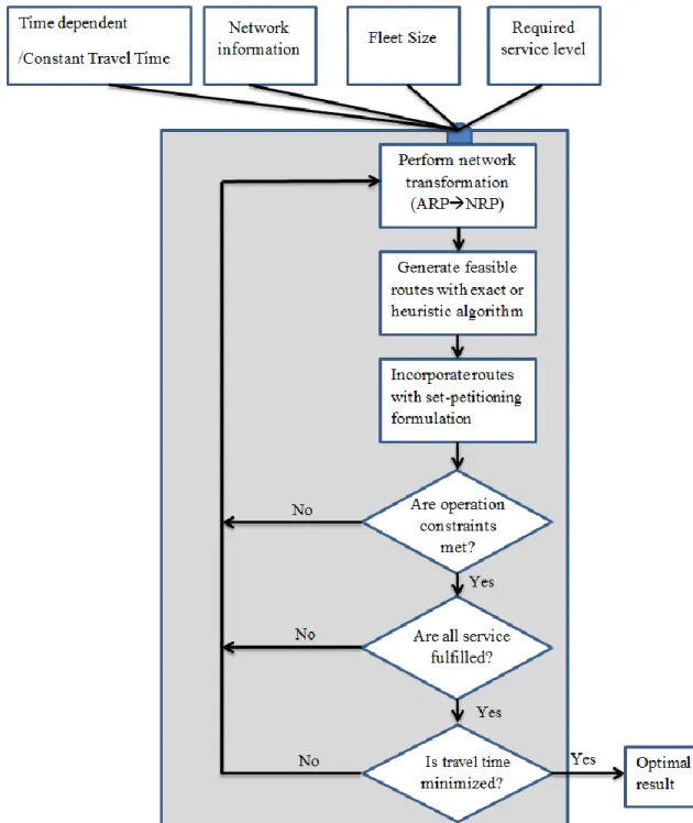
3.1 Implementation of model development ………. 45
3.2 The original network ……….. 49
3.3 The transformed network from the original network ………. 50
3.4 Temporal traffic speed distribution ……… 55
3.5 Corresponding travel time for a link of length 2 miles ……….. 56
4.1 Example of generating service routes ……… 62
4.2 An example of roulette wheel ……… 66
4.3 Example of one-point crossover ……… 67
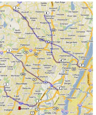
5.1 The study network for traffic data collection ………. 71
5.2 The transformed route network for traffic data collection ………. 72
5.3 Minimum required fleet sizes vs. various numbers of sample size ………... 80
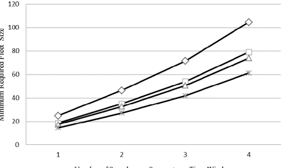
5.4 Minimum required fleet sizes vs. various time window durations ……… 81
5.5 Fleet size vs total vehicle travel time ………. 82
5.6 Example network of winter road maintenance ……….. 84
5.7 Example of plow tasks ………... 85
6.1 New Jersey snow sections and maintenance yards ……… 95
6.2 Selected snow sections in the northern New Jersey roadway network ………….. 97
6.3 Sample of the studied transportation network in ArcGIS ……….. 99
xv
(Continued)
Table Page
6.5 (a) Existing snow sections and maintenance yard in Sussex ………. 106
6.5 (b) Optimized service routes for Sussex ……… 106
6.6 Service route details ………... 106
6.7 Service routes developed for Scenario I ……… 109
6.8 Service routes developed for Scenario-II ………... 111
6.9 Cycle time distribution ………... 112
6.10 Deadhead travel distance distribution ……… 113
1
CHAPTER 1
INTRODUCTION
1.1 Background
Routing and scheduling vehicles to perform the required service within a transportation network play an important role in the area of transportation planning and engineering. It is challenging for transportation planners to represent real-life conditions closely with traditional modeling approaches either with strict assumptions that make them limited or not applicable in real-world application, or complex formulations that make them difficult and inefficient to be implemented. One practical aspect that needs to be addressed is the travel time variability. Most of the models for vehicle routing and scheduling reported in the literature assumed constant travel time by ignoring its variation. Unfortunately, constant travel time is a weak assumption for congested conditions that can result from recurring (e.g., congestion during peak hours, work zone, etc.) or non-recurring (e.g., accidents, vehicle breakdowns, etc.) events. Therefore, the optimal solution subject to constant travel time may be suboptimal or even infeasible for time-dependent cases (e.g., snow emergency salting and plowing operations).
Travel time is a fundamental measure in transportation planning and engineering, whose variability and reliability are always of concern to travelers and transportation professionals. With the rapid development of Intelligent Transportation Systems (ITS), traveler information (e.g., travel time and delay) can be delivered to motorists through various communication technologies deployed on the transportation infrastructure and in
vehicles. Many roadways have traffic sensors (i.e., inductive loops, acoustic sensors, etc.) for counting spatial as well as temporal traffic volume and speed, and apply new technologies (e.g., cell phones, GPS, and Bluetooth, etc.) for approximating travel times. In order to validate the travel time estimates with data collected by different sources, probe vehicles are commonly used for collecting ground truth O-D (Origin-Destination) based travel time. Because obtaining accurate O-D travel time for a transportation network with sufficient probe vehicles is expensive, it is desirable to develop a cost-effective data collection plan with optimized routes and schedules for vehicles considering practical constraints.
Vehicle routing and scheduling with time dependent travel time makes it possible to model the problem of winter road maintenance, where the timing of an intervention is of prime importance. If the intervention is too early or too late, the cost in material and time varies. In addition to the material cost, the state governments contract third-party trucks to support their operations during winter storms to make their operations more flexible and reduce truck maintenance cost. The payment rule used for these third-party trucks can be based on total travel time. In this case, the total travel time contributes majorly to total spending, which motivated this study to design efficient routes and schedules for winter maintenance operations to reduce the total cost while maintaining good level of service.
1.2 The Nature of the Problem
The nature of the research problem discussed in this study is a network optimization problem, involving efficient routing and scheduling of a number of vehicles engaged in
practical transportation applications (e.g., data collection, winter road maintenance) on a predetermined directed graph G=(V, A),where V is a set of nodes, and A is a set of arcs connecting pairs of nodes in V. It is assumed that A is partitioned into a subset of required arcs A1, and a complementary subset of arcs A2. A1 known as “requests” or “demands” must be serviced. The pickup and delivery locations are analogous to the start and end nodes of each arc. Because time windows are imposed for each arc belonging to A1, requiring vehicles to serve required arcs within pre-specified time periods based on the project needs. In other words, each “request” may occur in multiple time windows within a project duration (see Figure 1.1), which can be formulated as the arc routing problem with multiple time windows (Dumas et al., 1991 and Desroisers et al., 1995).
Figure 1.1 "Requests" at multiple time windows.
This study was considered in the context of the network optimization problem involving vehicle routing and scheduling. A generalized mathematical model was developed, which can be used to minimize either the total operating cost or travel time for vehicle routing and scheduling problems, subject to a set of practical constraints (e.g., limited budget, fleet size, number of demands, and project duration, etc.).
A set-partition approach was proposed to formulate the problem. Firstly, a number of promising feasible routes were generated by taking resource constraints or operational constraints into account. Secondly, these routes were treated as input to a mathematically formulated model that gives a solution of optimized routes and schedules that tells where and when to deploy vehicles. The exhaustive enumeration method was used to generate candidate routes for problems with a small size of demand. Then a genetic algorithm based heuristic was developed for solving problems with large size of demand. By using this efficient heuristic with adjustments, the proposed optimization model is able to solve the studied problem with consideration of time-dependent travel time.
1.3 Objective and Work Scope
Travel time and its variability are important indicators of roadway level of service. Various technologies (e.g., GPS, Bluetooth, etc.) have been widely applied for collecting speed data to approximate travel time. It is challenging to design a cost-effective plan including the routing and scheduling of vehicles to fulfill required service while considering time-dependent travel time. Because the nature of routing and scheduling vehicles for winter road maintenance makes the problem itself can be mathematically formulated as an Arc Routing Problem (ARP), thus the objectives of this study are:
1. To develop a mathematical model considering travel time variability for the winter road maintenance problem to minimize total vehicle travel time. Small size problems will be solved using an exact algorithm.
2. To develop an efficient solution algorithm to find good solutions for larger size problems, since the research problem is NP-hard.
3. To study the impact of travel time variability on vehicle routing and scheduling by comparing results obtained with constant travel time and time-dependent travel time.
To satisfy the above objectives, the nature of the routing and scheduling problem, its variants and solution algorithms were reviewed. Then the research problem was formulated and solved using the developed modeling approach and the solution algorithm. Later, two numerical examples based on applications of travel time data collection and winter snow plowing operation were provided to demonstrate the effectiveness of the developed model and solution algorithm. To extend this study’s applicability to address the impact of travel time variability, constant travel time inputs were replaced by time-dependent ones. A complete case study based on 41 snow Sections in the northwest area of New Jersey was undertaken to evaluate the performance of the proposed model in both the constant travel time and time-dependent travel time setting.
1.4 Dissertation Organization
This dissertation was organized into seven chapters. Chapter 1 introduces the background of travel time data collection and presents the research objective and work scope. Chapter 2 summarizes the efforts of previous studies related to vehicle routing and scheduling problems, solution algorithms and applications. Chapter 3 presents the model development with the set partition approach,which was used to mathematically formulate the studied problem considering travel time variability. Chapter 4 introduces the exhaustive enumeration and the genetic algorithm based heuristic for solving the mathematical model that was developed in Chapter 3. Chapter 5 presents two numerical examples on travel time data collection and winter road maintenance to demonstrate the
applicability of the present model. Chapter 6 presents a case study based on snow Sections in the state of New Jersey. Chapter 7 presents computational analysis by comparing results obtained by using the exact algorithm and results obtained by using the GA based heuristic. Finally, Chapter 8 concludes the findings of this study and suggests the directions of future research.
7 CHAPTER 2
LITERATURE REVIEW
This chapter discusses the literature review results in the area of vehicle routing and scheduling and its related variants and applications in winter road maintenance. In Section 2.1, the definition of Variability of Travel Time (VTT), its impact on vehicle routing and scheduling and the current technologies for travel time collection are reviewed. Later, the original problem of vehicle routing and scheduling is reviewed in the context of network optimization problem, which can be categorized and reviewed in details as two major related problems: Node Routing Problems (NRP) (Section 2.2) and Arc Routing Problems (ARP) (Section 2.3). The relationship between NRP and ARP and techniques of how one can be transformed to the other are discussed in Section 2.4. In Section2.5, research related to winter roadway maintenance is reviewed. After reviewing these problems, a brief discussion of solution algorithms including exact algorithms and heuristic algorithms are presented in Section 2.6. Finally, Section 2.7 summarizes the findings of the literature review.
2.1 Variability of Travel Time (VTT)
The Variability of Travel Time (VTT) in transportation systems has been the focus of many transportation agencies, because it affects transportation planning, design and operation, and system evaluation. Examples of planning and design applications include: 1) Develop transportation policies and programs; 2) Perform needs studies or assessments (Lyman and Bertini, 2008); 3) Rank and prioritize transportation improvements (Lyman
and Bertini, 2008); 4) Evaluate transportation improvement strategies (Chen et al., 2003); and 5) Calculate road user costs for economic analyses (Chen et al., 2003). VTT can result from traveler behaviors (i.e., departure time, route choice, and driving characteristics) of traffic mix (i.e., passenger cars, transit vehicles, and trucks) and the transportation network topology, geometry and traffic control. VTT has increasingly been recognized as a major factor influencing travel decision making and, consequently, serves as an important performance measure in transportation management (Recker et al., 2005). The Texas Transportation Institute’s Urban Mobility Report (2012) defined reliability and variability of travel time separately. Reliability is commonly used in reference to the level of consistency in transportation service; and variability is the amount of operating inconsistency. To quantify reliability and variability, travel conditions in the peak period were compared to free-flow conditions and two measures were defined: Travel Time Index (TTI) and Buffer Time. The TTI can be used in various systems with different free-flow speeds. Values of the TTI can used by the general public as an indicator of extra time spent in a transportation system during a trip. Buffer Time is the amount of extra time that must be allowed by a traveler to reach his or her destination on time in 95% of the time. Back in 2000, Florida DOT developed and documented the Florida Reliability Method. Similar to the Texas Transportation Institute’s definition of travel time reliability, they defined reliability on a highway segment as 95% of travel that takes no more than the expected travel time plus a certain acceptable additional time. These measures provide transportation planners and modelers a quantifiable basis to investigate and explore causes of travel time variability.
2.1.1 Impacts of VTT on Routing and Scheduling
VTT significantly impacts vehicle routing as well as scheduling when delivery times are heavily restricted by customers’ time windows and schedules. For example, Holguin-Veras et al. (2006) investigated the effects of New York City’s congestion pricing on commercial vehicles’ delivery schedules and found little changes because delivery times were set by customer time windows and schedules. It was also found that a large proportion of carriers do not worry about the toll increase change since customers are willing to take the extra cost rather than to compromise the scheduled delivery times. In contrast, carriers pay more attention on traffic conditions that could be interpreted as travel time variability.
Figliozzi (2010) analyzed the impact of congestion on commercial vehicle tours. The paper suggested that VTT is significant when the travel time between the depot and customers is long in relation to the maximum tour duration and when the routes are highly constrained by travel time. Also VTT impacts carriers’ productivity that can be measured in terms of tour time and distance required to serve a customer. Percentage of time driving and the average distance traveled per customer are usually used to indicate the efficiency of an individual tour because they are directly related to carriers’ operating cost. Quak and De Koster (2009) utilized a fractional factorial design and regression analysis to quantify the impacts of delivery constraints and urban freight policies. Their findings confirmed previous results from Holgun-Veras’s study showing that the cost impact of time windows is the largest for retailers who combine many deliveries in one vehicle round-trip. In summary, when a time window constraint for vehicle pickup and
delivery comes into consideration, VTT has a significant impact on vehicle routing and scheduling decisions.
Evidence on the behavioral response to VTT has also been obtained by analyzing route choice decisions. Abdel-Aty et al. (1993) analyzed state preference data from Los Angeles, CA, where respondents were provided with five hypothetical choices based on the traffic report accuracy. The degree of accuracy was described as: 1) extremely accurate, 2) very accurate, 3) somewhat accurate, 4) not very accurate and 5) not accurate at all. These choices gave the option of two alternative routes with different means and variances of travel time. The results revealed the important relationship between the use of travel time information and the propensity of route changes. From the commuters’ standing point, traffic conditions, perceptions of information accuracy and traffic variation were among the variables influencing the frequency of route changes based on en-route traffic information. From the planner’s standing point, problems involving vehicle routing and scheduling should take those variables into consideration.
Noland (2002) developed a schedule delay framework in a simulation experiment for a hypothetical network with two routes. By varying the degree of travel time variation due to non-recurring congestion on one route, it was possible to observe the changes on commuters’ route and departure time choices. The results showed that trips made by models with fixed schedules are subject to scheduling costs regardless of congestion with consequent implications. The change in travel activities is a major factor in valuing the costs and benefits of travel time variability. This work suggested that the modeling of route choice needs to consider scheduling effects if VTT becomes a major factor.
Recker et al. (2005) stated that VTT is increasingly being recognized as a major factor influencing travel decisions and, consequently, is an important performance measure in transportation management. The authors provide an analysis of segment travel time variability, which was first measured using a traffic database from GIS. The variability was measured from two different aspects, the first is the variability of day-to-day travel time, and the second one was within-day-to-day variability. The standard deviation and normalized standard deviation were used as measures of variability. Numerical experiments were carried out to examine the effects of route choice models on network assignment results. By incorporating travel time variability into the route choice models, the predictive capability of the route choice models was enhanced and could potentially lead to better means of reducing traffic congestion, wasteful travel, and loss of productivity, and at the same time, improve network capacity utilization and travel time reliability.
Hollander (2006) described two distinguishable modeling approaches based on modeling the attitudes of travelers to the unexpected day-to-day variability of travel times. In his study, the direct approach sees the extent of VTT as the variable that travelers react to, whereas the indirect approach claims that VTT effects are fully explained by trip scheduling considerations. In this, factors affecting bus users’ scheduling behavior and attitudes to VTT are investigated through a survey among bus users in the city of York, England. The results confirm that the influence of VTT on bus users was best explained indirectly through scheduling considerations. The considerations of scheduling should be addressed by taking VTT into consideration so that planners could better utilize the available bus fleet and reduce waiting time for bus users.
2.1.2 Technologies for Collecting Travel Time Data
The rapid progress of information technology (IT) may provide new insights to the understanding of traffic phenomena. Many technologies including the ITS probe vehicle have been used in travel time data collection. The Automatic Vehicle Identification (AVI) transponder [e.g., TRANSCOM’s System for Managing Incidents and Traffic (TRANSMIT)], which is located inside a vehicle and is used in electronic toll collection applications, is an example. This system utilizes antenna readers installed at regular intervals along the highway to identify the time when each transponder-equipped vehicle passes by. The detection of an equipped vehicle at successive readers downstream produces estimates of link travel times.
Various research studies and operational tests were conducted in regards to measure travel times through the use of electronic toll collection (ETC) system. Wright and Dahlgren (2001) discussed that ETC on the eight bridges crossing San Francisco Bay provided the means for a relatively simple and low cost system for measuring travel times on bridges and roads. Readers at various locations could recognize the toll tags used for ETC. The time of reading was recorded so that the time difference between when a vehicle passes one reader and another could be obtained. It was found that the application of ETC data improved facilities efficiency and reduced users delay. Saka and Agboh (2002) discussed the aggregated impact of ETC (also called M-Tag) deployment at three toll plazas in the Baltimore Metropolitan Area. The toll plazas were treated as multi-server queuing systems. The delay as well as travel time data were used to estimate mean vehicular travel speed at the toll facilities. The analysis involved the development of
simulation and deterministic models used to generate traffic flow parameters, including speed and driving cycles for the study areas.
GPS Based Probe Vehicle:
In this section, the GPS based probe vehicle was mainly discussed in terms of the technology itself, its advantages and disadvantages, and its popularity in real practice of travel time data collection. One of the key applications of IT to traffic and transport analysis is the identification of the location of moving objects using the global positioning system (GPS). It is expected that detailed traffic analysis could be carried out using these data. Zito et al. (1995) were the first to address the use of GPS data for traffic engineering. They discussed the accuracy of the GPS and its potential for traffic analysis, and suggested that geographical information systems (GIS) could be used efficiently for managing the data obtained by the GPS. A study that estimated VTT on New Jersey (NJ) highways was conducted by collecting travel times with probe vehicles carrying GPS devices (Chien et al., 2010). The results include estimated travel time and its variability on selected NJ highways by departure time of day and day of the week. The travel time data were collected through the use of an in-vehicle navigation device equipped with a GPS-receiver. The use of GPS-based link/path travel time data collection could produce the corresponding distributions and buffer index to assist real-time traffic operations (e.g., signal timing) traveler information (e.g., real-time route planning), and transportation short term and long term planning (e.g., infrastructure and traffic management strategies). Number of Probe vehicles:
Travel times are generally estimated by roadside detectors. Travel time cannot be observed on a road without any onsite observation instruments, although some estimation
techniques have been proposed. The probe vehicle approach is one efficient method of collecting LOS information and data about the source of traffic congestion. The reliability of probe vehicle data for estimating the travel time should be investigated. Karthik et al. (1996) implemented an algorithm to determine the number of probe vehicles required for reliable travel time measurement by using a simulation of the Sacramento network for the morning peak period. The results indicated that the number of probe vehicles required increases nonlinearly as the reliability criterion is made more stringent. More probes are required for shorter measurement periods. As the desired proportion of link coverage in the network increases, the number of probes required increases. With a given number of probes a greater proportion of freeway links than of major arterials can reliably be covered. Probe vehicles appear to be an attractive source of real time traffic information in heavily traveled, high speed corridors such as freeways and major arterials during peak periods, but not recommended for coverage of minor arterials or local streets during off-peak hours.
Lee et al. (2006) examined the relationship between the number of probe vehicles and the travel time collection reliability using both simulated and field data. Their results suggested that the operational characteristics of probe vehicles are very important when constructing a reliable information system that needs to meet network coverage requirements. Cheu et al. (2002) also discussed the population and size of probe vehicles using a simulation-based analysis. They concluded that the improvement in the accuracy of link speed estimation diminishes when the probe vehicle population in the network reaches the threshold of 15% of the total network traffic network volume. They further concluded that to achieve an absolute error in the estimated average link speed of less
than 5.0 km/h at least 95% of the time, there should at least 4 to 5% active probes in the total network traffic volume, or at least 10 probes that have successfully traversed a link. As stated in the above studies, viewing the travel time data collection from a statistical perspective, having enough probe vehicles is crucial because the sample size determines the accuracy of the travel time estimation. But standing from the viewpoint of the cost control, it is costly to schedule and route vehicles to collect enough data samples without compromising data accuracy. Thus, it is important to develop a mathematical model to optimize routes and schedules based on minimum cost.
2.2 Node Routing Problem
Node routing problems try to find the minimum cost routes that service the nodes in the network. There are two main problems in this category, one is the travelling salesman problem (TSP), which does not have the capacity constraint, and the other is the vehicle routing problem (VRP), which considers the capacity constraint. In the classical node routing problem if there is only one vehicle and there is no capacity constraint, the problem simplifies into a traveling salesman problem. This section focuses on the capacitated VRP and its variations.
2.2.1 Vehicle Routing Problem with Pickup and Delivery (VRPPD)
The classical VRP can be described as follows: A fleet of m capacitated vehicles localized at one or more depots have to serve n customers with demand d. The problem is to find the minimum cost route for all vehicles so that all customer demands are satisfied. The VRP with pickup and delivery (VRPPD) is an extension of VRP. In addition to the traits of VRP each customer i now has both an origin (pick-up point), as well as a
destination (drop-off point) and the demand. Typical applications can be found in the fields of parcel and para-transit services. The VRPPD is a generalization of the classical VRP, which also belongs to a larger family of pickup and delivery problems (PDPs). One can distinguish between three well-known types of pickup and delivery problems that have been studied in the literature. 1) One is the single-commodity PDP in which a single type of good is either picked up or delivered at each node (Hernandez-Perez and Salazar-Gonzalez, 2004). This is the case, for example, when an armored vehicle transports money between the branch offices of a bank. 2) Another variant is the two-commodity PDP where two types of goods are considered and each node may act as both a pickup and a delivery node (Angelelli and Mansini, 2002). This problem arises in beer or soft drink delivery where vehicles deliver full bottles and collect empty ones. A variant of this problem is the VRP with backhauls in which all deliveries must be performed before any pickup. 3) Finally, the n-commodity problem occurs when each commodity is associated with a single pickup node and a single delivery node. This is the case when passengers or goods must be transported from an origin to a destination.
2.2.2 Vehicle Routing Problem with Time Windows (VRPTW)
Because most practical applications of the VRPPD include restrictions on visiting time at each location that may be visited by a vehicle, it is convenient to present a more general variant of the problem, called the VRPPD with time windows (VRPPDTW). The VRPPDTW is NP-hard since it generalizes the TSP that is also known to be NP-hard (Garey and Johnson, 1979). With the presence of time windows, even finding a feasible solution to the problem is NP-hard since the feasibility problem for the TSP with time windows is itself NP-complete (Savelsbergh, 1985). Savelsbergh and Sol (1995)
considered a more general formulation of the pickup and delivery problem and reviewed the relevant literature on this problem. A more recent survey on pickup and delivery problems with time windows was also prepared by Desaulniers et al. (2001). In this study, empirical applications in winter road maintenance and travel time data collection can have multiple time windows on each demand that located on either arcs or nodes.
Time windows can be classified into two types: hard time windows (HTW) and soft time windows (STW). In the first case, if the vehicle arrives early, it must wait until the lower bound of the window, and it is strictly forbidden to arrive late. In the case of STW, the violation of the constraint is permitted but leads to an objective function penalty. As discussed by Chiang and Russell (2004), VRP with soft time windows (VRPSTW) has been practically applied for the following reasons: 1) relaxing HTW constraints to reduce total cost without compromising customer satisfaction; 2) relaxing unnecessary HTW constraints for particular applications (e.g. the delivery of fuel/gas to service stations); 3) dealing with issues related to travel time uncertainty; 4) solving VRPHTW with proper penalty setups. The solution of VRPSTW was used as an alternative answer when the solution of VRPHTW is infeasible.
Replacing HTW constraints with STW ones will increase computation time because of the increase in feasible solution spaces. Thus, an efficient solution algorithm is desirable to improve the computational efficiency. Qureshi et al. (2009) presented a new column-generation-based approach to find exact optimal solutions for vehicle scheduling problems with STW constraints. An elementary shortest path problem with resource constraints and late arrival penalty was solved as a sub-problem. It was found that the VRPSTW solution results in fewer routes and lower cost while a late arrival
penalty has a small impact on total cost. Figliozzi (2010) developed an iterative route construction and improvement algorithm for solving VRPSTW, which was able to accommodate general cost and penalty functions. Experimental results indicated that the average run time performance was significantly improved. Even though the increased computation time can be handled by some solution algorithms, there is still case that HTW is more preferable. In winter gritting operations, where a subset of road segments must be serviced at a cost that depends on the time service begins, if the intervention is too late, the cost in material and time sharply increases. Therefore, planners would rather have vehicles arrive early than fine vehicles for arriving late.
2.2.3 Vehicle Routing Problem with Time-dependent Travel Time
Most of the VRP models and their solution approaches assume that all characteristics are independent of the time of day. Therefore, these models may have problems to deal with real-life applications where travel time can be influenced by congestion or incidents occur on the road network. The literature related to vehicle routing with time-dependent travel times is relatively scarce.
Malandraki and Daskin (1992) examined both the time-dependent vehicle routing problem (TDVRP), and the time-dependent traveling salesman problem (TDTSP) which is a special case of the TDVRP, where the feet size is equal to one. They provided mixed integer linear programming formulations that included capacities and time windows constraints. The travel times were computed using step functions. The travel time between two customers or between a customer and the depot depends on the travel distance and time of day. The Nearest-neighbor (greedy) heuristics for TDTSP and TDVRP without time windows were proposed, as well as a branch-and-cut algorithm for
solving small problems with 10 to 25 nodes. In Malandraki and Dial’s following work (1996), a dynamic programming algorithm was developed to solve the TDTSP. Although it was argued that this algorithm can handle many different types of travel time functions, no results comparison was done between different types of travel time functions. Results were only reported for step functions found in their previous work (1992).
Hill and Benton (1992) considered a TDVRP (without time windows) and proposed a model based on time-dependent travel speeds. In their formulation, the travel time on a given link is dependent on the average travel speed during the period that a vehicle starts travelling. Computational results were reported on a small example with a single vehicle and five locations. The authors implemented a simple greedy heuristic for the multi-vehicle traveling salesman problem with capacity constraints and no time windows for a city with 210 locations. A validation of the model was conducted in a commercial courier vehicle scheduling system and was judged to be very useful by users in a number of different metropolitan areas in the United States.
Donati et al. (2008) considered variable traffic conditions in VRP to perform realistic optimization. TDVRP consists of finding optimal routes by considering the time it takes to traverse each given arc depending on the time of day travel starts. This variant of the classic VRP is motivated by the fact that in urban contexts variable traffic conditions play an essential role and cannot be ignored in order to perform a realistic optimization. The paper showed that when dealing with time constraints, like hard delivery time windows for customers, the known solutions for the classic case become unfeasible and the degree of unfeasibility increases with the variability of traffic conditions.
The TDVRPis more difficult to model and to solve than the VRP with constant travel time. The major issue is how to model the variation of travel time during a certain time period. Available models often discretized a time period into a limited fixed number of time intervals (e.g., morning, midday and afternoon) with a distinct associated fixed mean speed. Ichoua et al. (2003) used a model based on discrete travel speeds by adding correction factors to model congestion. It is a simple way to take time-dependency into account by working with time-dependent travel speeds and to adjust the speed when the vehicle crosses a boundary between two time periods. In contrast with the formulation proposed by Hill and Benton (1992) where travel speeds corresponded to time periods and nodes, the travel speeds were associated with different time periods and arcs in Ichoua et al.’s study. This reduced the computational effort at the cost of storing speed data. Hill and Benton’s model was implemented in a static and a dynamic environment, respectively. The results showed that the time-dependent model provided significant improvement over the model with fixed travel times, which indicated the usefulness of time-dependent travel speed information.
Donati et al. (2006) expressed the total distance between any two nodes in terms of the time taken to traverse an arc. Travel speed was inversely proportional to the time taken to traverse the distance. A step function was used for representing the speed distribution, from which the travel time distribution was derived. By applying this travel speed modeling approach to a real road network with 1522 nodes and 2579 arcs, the authors concluded that the time dependent models can provide a better modeling of travel time when variable traffic conditions have a considerable influence on travel time. In general, time dependent travel time can be modeled in two ways: deterministically or
stochastically (Van Woensel et al., 2008). In the deterministic case, the travel time is known in advance. The travel time is then a function of distance and mean speed. For instance, Ichoua et al. (2003) considered three distinct time periods (where the first and third periods stand for the morning and evening rush hours, respectively, and the second period corresponds to the middle part of the day) and three different types of road links. This approach has been implemented within a parallel Tabu search developed by Taillard et al. (1995) for the fixed travel time version. It provided a simple way to take time-dependency into account by working with time-dependent travel speed that could be obtained from different sources of traffic data collection.
In the stochastic time-dependent models, the solution procedure takes into account the stochastic nature of travel time. Travel time is the result of taking into account not only mean travel time but ideally the travel time distribution itself. As the travel time distribution is derived from the speed distribution and the known distances, the approach requires realistic speed distributions. He et al. (2005) indicated that although mean and variance contain the most important information about path travel time, finding the single route with expected shortest travel time is not appropriate for routing when planners are not risk neutral. The entire travel time distribution contributes to the routing choice. A stochastic model usually involves two stages. In the first stage, a route is planned a priori, followed by a realization of the random variables. In the second stage, a recourse or corrective action is then applied to the solution of the first stage. The cost/saving generated though the recourse action may have to be considered when designing the first stage solution.
In this dissertation, to include time-dependency into vehicle routing and scheduling, a predefined service time period was discretized into a limited fixed number of time intervals (e.g., 15-minute intervals) with a distinct associated fixed mean speed that was extracted from historical speed data or proper estimation. Future work will be focused on the integration of the real-time information (traffic conditions) and the speed profile provided by historical data. The general idea is to modify in real time, the speed profiles to accommodate traffic and thus to provide more realistic travel times.
2.3 Arc Routing Problem
The arc routing problems belong to another subset of the network optimization problems. While in node routing problems one tries to visit the nodes of the network, in arc routing problems the objective is to traverse the arcs of the network. The Chinese Postman Problem (CPP) and the Rural Postman Problem (RPP) are two popular arc routing problems.
CPP was simply stated by Kwan (1962) as the problem of finding the shortest walking distance for a mailman who has to cover his assigned segment before returning to the post office. Two extensions of CPP were described as follows. One is the windy postman problem (WPP), in which the underlying network is an undirected graph, but the cost of traversing an arc depends on the direction of travel. Another form of CPP is the hierarchical CPP where a precedence relation is defined on arcs of the graph, and the order in which the arcs are serviced must respect this relation. CPP can be viewed as the counter part of the traveling salesman problem in the category of arc routing problems. The capacitated CPP is a counterpart of the VRP in the ARP and deals with a more
realistic case than CPP. Given the demand for each arc that must be satisfied by vehicles with given capacities, find a set of cycles that all pass through a domicile and satisfy demands at minimal total cost. Just like that CPP is more likely to arise in urban areas, RPP is commonly associated with mail delivery in rural areas. There are a number of areas whose set of streets has to be serviced by a postman, and the other set of links between those areas that do not have to be served, but may be used for traveling between those areas. This problem is to find the minimum cost route to service those arcs that must be served.
Christofides and Beasley (1984) introduced the periodic arc routing problem (PARP), the problem of designing vehicle routes to meet required service levels for customers and minimize distribution costs over a given several-day period of time. A typical PARP in real life is the waste collection problem. Waste management companies gather statistics and know the average daily waste production in each street. This amount depends on the region, the population and the habitat. Apartment blocks in town centers cannot store waste for a long time in their basements so that it needs to be collected everyday generally. Houses in residential areas may keep waste for a few days in a container located in a garage or a garden and do not need a daily removal. This is why the collection process must be planned over a multi-period horizon. In practice, planners translate these waste productions into one service frequency for each street, for instance “everyday” or “twice a week”. Like location and districting, these computations depend upon the strategic decision level, because frequencies must remain constant for at least one year, to avoid upsetting the residents. It is assumed in the sequel that all strategic decisions have been already taken.
PARP in waste collection consists of selecting for each street a number of treatment days equal to its frequency (tactical decisions), and then of computing the trips for the streets assigned to each day (operational decisions). Obviously, the total cost over the horizon depends on this combination of assignment and routing decisions. Waste collection is just one example. A similar organization can be found in other applications like winter gritting, sweeping, inspection of power lines, or spraying herbicides on rails or roads to kill weeds.
2.4 Transformation between NRP and ARP
It can be shown that a VRP can be transformed into an ARP, and that an ARP can be transformed into a VRP, making the two classes of problems equivalent. For transformations of ARP into VRP, the resulting VRP instance requires either adjustment of variables or the use of arcs with infinite cost. In this Section, the relationship between NRP and ARP is reviewed.
2.4.1 Transformation of NRP to ARP
Relatively Very few studies addressed the transformation from NRP to ARP, because the transformation usually is accompanied by a significant increase in the size of the problem. Golden and Wong (1981) showed how NRP can be transformed into a capacitated ARP by slitting each nodes into two nodes joined by an arc, and by assigning the original node demand to that arc. Ghiani and Improta (2000) developed an efficient transformation of VRP into a capacitated ARP with only increasing the number of nodes by not much. The number of nodes increased after transformation was dependent on the number of multiple membership nodes in the original problem. They proposed a transformation that can be
divided into three main stages. In the first stage, the general problem was transformed to a general TSP having mutually exclusive node sets. In the second stage, the intraset arcs were eliminated. In the third stage, the problem was transformed to a clustered TSP and then finally into a standard TSP. The resulting TSP has an arc and arc cost structure, which can be optimally solved by an approach based on integer linear programming. 2.4.2 Transformation of ARP to NRP
The field of arc routing is gaining momentum. However, since more literature is available on Node Routing Problems, some have ventured to turn ARP into VRP. The first and most generally used method for converting ARP into VRP was done by Pearn et al. (1987). They transformed the capacitated ARP into a capacitated VPR by replacing each arc with positive demand with three vertices, each having a demand equal to one third of the original demand. In this formulation the distances between vertex pairs were defined to enforce the constraint that a customer can only be visited by a single vehicle in the VRP and to guarantee that the three arcs appear consecutively on the same route in any capacitated VPR solution. Laporte (1997) transformed several types of ARP such as the Rural Postman Problem. Instances involving up to 220 vertices, 660 directed arcs and a few undirected arcs were solved to optimality on low density graphs. The transformation includes three steps:
1. Replace each edge by two arcs;
2. Create a transformed network. The nodes in the transformed network are the arcs in the original network; the arcs in the transformed network are the length of the shortest path between two arcs in the original network;
However, the transformation is regarded as unpractical, since an original instance with r required edges was turned into a CVRP over a complete graph with 3r+1 vertices. Longo et al. (2004) proposed a similar transformation that reduces this graph to 2r+1
vertices, with the additional restriction that r edges were already fixed to 1. Using a recent branch-and-cut-and-price algorithm for the CVRP, it was observed that it yields an effective way of attacking the CARP and computational experiments obtained improved lower bounds for almost all open instances. But, the transformation entails certain drawbacks summarized by Letchford and Oukil (2009):
1. A huge amount of memory is needed to perform the transformation. 2. The transformation method is not suitable for all types of graphs.
To address these two drawbacks, it is worth noticing that as the information techniques have been developing in a fast pace, the memory capacity should not be a barrier for transforming ARP to VRP. Also, with appropriate adjustments on network graphs, the applications of ARP in waste collection, winter plowing and spreading can be formulated in the context of VRP.
2.5 Vehicle Routing in Winter Road Maintenance
VRP is one of the most well studied problems in operations research, both in real life problems and for scientific research purposes. Many practical transportation problems including the winter road maintenance routing problem can be formulated as a VRP. Winter road maintenance operations involve challenging vehicle routing that can be addressed using operations research (OR) techniques. Key problems such as routing trucks and specialized vehicles for spreading chemicals and abrasives on roadways, snow
plowing, and snow disposal, all of which are undertaken in a difficult and dynamic operating environment with strict level of service constraints. There is an extensive literature of academic research on various issues related to the planning, design and management of winter road maintenance operations summarized by Perrier et al. (2006a,b, 2007a,b).
2.5.1 Vehicle Routing Problems for Spreading
Consider a road network consisting of a set of predetermined maintenance segments with each representing an itinerary that a service vehicle may follow. A fleet of vehicles is available to provide winter maintenance services such as salting during a snowstorm event. The problem is to develop an operation plan for the available service vehicles that specify a route assignment to take into account the following requirements:
1) The total operating cost is minimized; 2) The total service time is minimized;
3) The level of service for the network is maximized;
4) Total negative environmental effects (e.g., salt usage) are minimized.
Early studies generally formulated the routing problem related to spreading operations as ARP. Evans and Weant (1990) formulated salt spreading operations as the capacitated ARP and used the path-scanning algorithm to search for the optimal solution that satisfied the constraints of maximum service time for spreading completion, maximum route duration and vehicle capacities. Campbell and Langevin (2000) provided a detailed description of the snow removal and disposal operation in Montreal. They listed major arc routing theories, solutions and applications related to snow operations. These problems include site location, Section design, Section assignment, fleet mix and
routing. An integer programming formulation for snow disposal site location and the vehicle assignment problem was given.
Compared to early studies, researchers gradually incorporated more practical constraints and techniques into their models. Thus, the spreading problem cannot be only limited to the context of ARP. To reduce the operation cost that is dominated by total travel distance or total travel time of the entire fleet, Haghani and Qiao (2001) developed a model that incorporated the constraints of maximum route distance and truck capacities to optimize snow emergency routes for Calvert County, MD. Later, the model was enhanced (2002) by considering the link continuity constraint into the optimization processes. A heuristic approach was applied, which decomposes the problem into two components: “allocation of road Sections to salt spreaders” and “vehicle routing”. In the first component, the network transformation technique was used to convert an ARP to a NRP, and the minimum spanning tree formulation was used to calculate the minimum required fleet size to complete the entire spreading operation; and in the second one, the total deadhead cost was minimized by optimizing routes with the fleet size obtained from the first component.
Yu and Chien (2013) applied a similar network transformation technique to formulate a routing problem related to anti-icing and de-icing operations as a NRP. The objective was to minimize the service time needed for anti-icing/de-icing operations, subject to truck capacity, truck operating speed and fleet size constraints. After the vehicle routing network was converted from an ARP to a NRP, the study vehicle routing problem can be solved via dynamic programming (DP). The solution approach was tested
on a general network with practical operational data. The results were promising and computationally efficient.
In summary, despite of the difficulty of routing and scheduling vehicles for road maintenance, recently proposed models tended to take into account a larger variety of problem characteristics (e.g., roadway characteristics, snow sectors, level of service) arising in real-world applications. Recent developments in modeling and algorithmic tools, the increased performance of computers, and the increased desire from state and local agencies to reduce expenditures on winter road maintenance operations, while maintaining or enhancing service levels and minimizing environmental impacts, all motivate the more widespread use of optimization models.
2.5.2 Vehicle Routing Problems for Snow Plowing
Plowing operations involve a number of VRP where streets or roads have to be traversed by plows or trucks. The plow routing and scheduling problems consist of determining a set of routes, each traveled by a vehicle that starts and ends at its own depot, such that all road segments are serviced, all the operational constraints are satisfied, and the global cost is minimized. Similar to routing problems related to spreading operations, routing problems related to plowing operations were generally formulated as arc routing problems.
Marks and Stricker (1971) modeled the plow routing problem as a multiple vehicle CPP, which is a special case of ARP. The authors attempted to minimize deadhead distance while respecting the service requirements and vehicle capacity constraints. Haslam and Wright (1991) and Wang and Wright (1994) developed a maintenance decision support system for the Indiana Department of Transportation
planners to determine snow plowing routes with minimized deadheading, service time window violation and the total distance of class upgraded road segments. The system can handle plow routing problems with service time windows, class continuity and class upgrading constraints.
Perrier et al. (2008) proposed a formulation and two solution approaches based on mathematical optimization techniques for the routing of snow plowing vehicles in urban areas. Given a district and a single depot where a number of plows are based, the problem is to determine a set of routes, each performed by a single vehicle that starts and ends at the district’s depot, such that all road segments are serviced while satisfying a set of operational constraints and minimizing a service completion time. The model contained general precedence relation constraints with no assumption on class connectivity, different service and deadhead speed possibilities, and vehicle road segment dependencies. The author proposed a model based on a multi-commodity network flow structure to impose the connectivity of the route performed by each vehicle, as well as constraints to model a hierarchical objective. The problem was solved by means of two constructive algorithms. The first one constructed several routes in parallel by sequentially solving a multiple vehicle rural postman problem with side constraints. The second was a cluster-first, route-second algorithm, which first determines a partition of the arcs into clusters, each having approximately the same work load. A hierarchical rural postman pr