Applying fractional order PID to design TCSC-based damping controller in coordination with automatic generation control of interconnected multi-source power system

Full Length Article

Applying fractional order PID to design TCSC-based damping controller

in coordination with automatic generation control of interconnected

multi-source power system

Javad Morsali, Kazem Zare

⇑

, Mehrdad Tarafdar Hagh

Faculty of Electrical and Computer Engineering, University of Tabriz, Tabriz, Iran

a r t i c l e i n f o

Article history: Received 31 January 2016 Revised 13 May 2016 Accepted 5 June 2016 Available online xxxx Keywords:

Automatic generation control (AGC) Thyristor controlled series capacitor (TCSC) Fractional order proportional-integral-differ ential (FOPID)

Generation rate constraint (GRC) Interconnected multi-source power system Dynamic performance

a b s t r a c t

In this paper, fractional order proportional-integral-differential (FOPID) controller is employed in the design of thyristor controlled series capacitor (TCSC)-based damping controller in coordination with the secondary integral controller as automatic generation control (AGC) loop. In doing so, the contribu-tion of the TCSC in tie-line power exchange is extracted mathematically for small load disturbance. Adjustable parameters of the proposed FOPID-based TCSC damping controller and the AGC loop are optimized concurrently via an improved particle swarm optimization (IPSO) algorithm which is reinforced by chaotic parameter and crossover operator to obtain a globally optimal solution. The powerful FOMCON toolbox is used along with MATLAB for handling fractional order modeling and con-trol. An interconnected multi-source power system is simulated regarding the physical constraints of generation rate constraint (GRC) nonlinearity and governor dead band (GDB) effect. Simulation results using FOMCON toolbox demonstrate that the proposed FOPID-based TCSC damping controller achieves the greatest dynamic performance under different load perturbation patterns in comparison with phase lead-lag and classical PID-based TCSC damping controllers, all in coordination with the integral AGC. Moreover, sensitivity analyses are performed to show the robustness of the proposed controller under various uncertainty scenarios.

Ó2016 The Authors. Production and hosting by Elsevier B.V. on behalf of Karabuk University. This is an open access article under the CC BY-NC-ND license (http://creativecommons.org/licenses/by-nc-nd/4.0/).

1. Introduction

Lately, fractional calculus has received considerable attention in engineering researches with a growing interest in applying fractional order controllers (FOC)[1]. Fractional calculus extends the ordinary differential equations to fractional order differential equations, i.e. those having non-integer powers of differentials and integrals. Fractional order proportional-integral-differential (FOPID) is a generalization of integer order PID (IOPID) controller employing fractional calculus. The FOPID controller, so-called PIkDl, is a popular and suitable fractional order structure that has been investigated comprehensively in recent literature [2]

due to its flexibility to satisfy design specifications and hence to control a system in a wide dynamic range. Fractional calculus can comprise both modeling of a system with fractional order dynamics and performance control of linear dynamic systems by

the FOC[3]. The design of an FOPID controller involves finding of proportional gain, integrating gain, differential gain, integrating and differential orders which are not necessarily integer. Different evolutionary algorithms such as bacterial foraging [4], non-dominated sorting genetic algorithm II (NSGA II) [5], particle swarm optimization (PSO)[6], and chaotic ant swarm (CAS) algo-rithm[7,8]are used in tuning of the FOPID controllers. Recently, utilizing FOCs, especially the FOPID controller, have received more attentions in electrical power engineering topics for power system control objectives due to the progresses in computational power that permits simulation and implementation of the FOC with suffi-cient accuracy. In[6–8], the FOPID controller is used as an auto-matic voltage regulator (AVR). It has been shown that FOPID controller surpasses IOPID counterpart in improving the system dynamic performance due to its flatness in the phase margin contribution with wider bandwidth. Also, sensitivity analysis shows that the FOPID-based AVR can provide better robustness performance than the classical IOPID under uncertainties in system parameters and wide range of operating conditions[5,8].

In automatic generation control (AGC) studies, it is aimed to maintain the frequency and tie-line power deviations as near as

http://dx.doi.org/10.1016/j.jestch.2016.06.002

2215-0986/Ó2016 The Authors. Production and hosting by Elsevier B.V. on behalf of Karabuk University. This is an open access article under the CC BY-NC-ND license (http://creativecommons.org/licenses/by-nc-nd/4.0/).

⇑ Corresponding author.

E-mail addresses:[email protected] (J. Morsali), [email protected] (K. Zare),[email protected](M. Tarafdar Hagh).

Peer review under responsibility of Karabuk University.

Contents lists available atScienceDirect

Engineering Science and Technology,

an International Journal

j o u r n a l h o m e p a g e : w w w . e l s e v i e r . c o m / l o c a t e / j e s t c h

possible to the minimal limits or even theoretically, in zero. Differ-ent integer order controllers (IOCs) such as the IOPID, proportional-integral-double differential (PIDD), and proportional-integral-double differential (IDD) have been used widely as secondary load frequency controller (LFC) so far[9–11]. In[4,12,13], the FOPID controller is used as sec-ondary load frequency controller (LFC) in AGC of power system and its dynamic performance is compared with several integer order controllers. It has been demonstrated that the FOCs outperform the IOCs in performance enhancement of the AGC system. The main advantage connected with the FOPID controller is that it contains two more adjustable parameters than the IOPID controller. Due to two more degrees of freedom, the FOPID controller supplies more flexibility and power to realize the design objectives of a control system. Hence, it brings better opportunity to adjust the system dynamics in addition to the less sensitivity to changes in parame-ters of the controlled system[4,12,14].

Applying flexible alternating current transmission system (FACTS) based controllers in interconnected power systems is an effective solution to improve the dynamic performance of the AGC system[11]. Due to fast dynamic responses, the series FACTS controllers such as thyristor controlled phase shifter (TCPS), static synchronous series compensator (SSSC), and interline power flow controller (IPFC), and thyristor controlled series capacitor (TCSC) have been employed in the tie-line of interconnected power sys-tems to damp the area frequency and tie-line power oscillations

[14–16]. The TCSC is a high-performance and cost-effective series FACTS that has a significant practical background. Recently, a new dynamic modeling and control method of the TCSC applicable in AGC is presented in[15]. It is proved that when the TCSC is added in series with the tie-line along with the AGC, the dynamic performance of the system is improved greatly. In order to imple-ment the TCSC-based damping controller, a 5th order approxima-tion of the Taylor series expansion has been used in [15,16]. Deciding on an appropriate approximation order is challenging. In fact, a compromise is established between the complication of the controller realization and its accuracy. This can be interpreted as a drawback for the suggested TCSC damping controller since the employed method uses approximation and lacks any precise model for the TCSC damping controller. In [17,18], a precise dynamic modeling and control of the TCSC in the AGC studies have been presented which has some good points over the approximated method. However, the contribution of the TCSC in the tie-line power flow exchange has not been presented independently. In the current paper, an attempt is made to present a new dynamic model and control method for the TCSC in which the tie-line power flow exchange is stated clearly in the mathematical formulations with and without the TCSC.

Literature survey shows that the FOCs have not been employed in the design of any FACTS-based damping controllers applicable in the frequency control studies, till now. Often, the phase lead-lag structure has been used in the design of the FACTS-based damping controllers[15,16,19]. So, employing of the FOPID in the proposed TCSC damping controller is a new idea which is going to be inves-tigated in this paper. The proposed FOPID-based TCSC damping controller in coordination with AGC loop can participate effectively in damping of the area frequency and tie-line power oscillations in an interconnected power system. Regarding above survey, the main contributions of this paper can be listed as:

(i) A new application for the FOPID is proposed to apply in the TCSC damping controller to improve the frequency stability. (ii) A new formulation for the tie-line power deviation in the

presence of the TCSC is extracted.

(iii) A new and precise TCSC damping controller is proposed which is advantageous in comparison with the previous techniques.

(iv) The proposed controller is optimized using an improved PSO algorithm which is reinforced by chaotic parameter and crossover operator to obtain global optimal solution. (v) The proposed control strategy is evaluated on an

intercon-nected multi-source power system in which the physical constraints of the GRC nonlinearity and GDB effect is taken into account for a challenging realization.

(vi) The dynamic performance of the proposed controller is com-pared with the PID and phase lead-lag type counterparts under step, sinusoidal and random load perturbation patterns.

(vii) Sensitivity analyses are performed to show the robustness of the proposed controller under wide range of operating con-ditions and various uncertainty scenarios.

2. Investigated power system

The case study is a two-area interconnected multi-source power system with reheat thermal, hydro, and gas generations in each control area [11]. Fig. 1 depicts the transfer function model of the power system. The parameters of hydro, reheat thermal, and gas units are described in Fig. 1 and are given in

[15]. The physical constraints of generation rate constraint (GRC) nonlinearity and governor dead-band (GDB) effect should be taken into account to challenge the effectiveness of any employed controller and to obtain precise and realistic results

[10]. The GDB and GRC restrict the instantaneous reaction of the generators to modify disturbances. In order to obtain an accurate realization and valid insight of the AGC problem, it is important to take into consideration the multi-source power generations in each control area and the physical constraints in the thermal and hydro units[10,11,14,20].

3. A review of fractional calculus

Fractional calculus is a generalization of integer order integral and differential to a fractional order operatoraDat whereaandt

denote the limits of the operation and

a

denotes the fractional order which is a complex number[1]. The fractional order operator is defined as: aDat ¼ da=dta Rð

a

Þ>0 1; Rð

a

Þ ¼0 Rt aðd

s

Þ a_{; Rð}

a

Þ<0 8 > < > : ð1Þ

There are various definitions and approximations for fractional derivative and integral such as the Grunwald–Letnikov definition, the Riemann–Liouville (R–L) definition, the Caputo definition, the Carlson approximation, the Matsuda approximation, and continued fraction expansion (CFE) method [2,5]. For example, the widely used R–L definition for fractional order differential is given by[4]: aDatfðtÞ ¼ 1

C

ðn

a

Þ dn dtn Zt a ðt

s

Þna1_fð

s

Þd

s

ð2Þ

where n1>

a

Pn; nis an integer number, and C() is Euler’s gamma function. The fractional order integral is given by: aDatfðtÞ ¼ 1

C

ð

a

Þ Z t a ðt

s

Þa1_fð

s

Þd

s

ð3Þ

For simplicity, Laplace transform is routinely employed to explain the fractional or integer order differentiation. For fractional order of

a

(0 <

a

< 1) in general, the Laplace transformation of the R–L fractional derivative or integral is given by:

LfaDatfðtÞg ¼saFðsÞ

Xn1

k¼0

sk

aDatk1fðtÞjt¼0 ð4Þ Under zero initial conditions forn1P

a

<n:

LfaDtafðtÞg ¼saFðsÞ ð5Þ whereL{f(t)} denotes the Laplace transformation. This signifies that when zero initial conditions are considered, the dynamic responses of a system described by fractional order differential equations turns to transfer functions with fractional orders of ‘‘s” (Laplace operator).

4. A new tie-line power flow exchange model considering TCSC in series with the tie-line

Precise modeling of the TCSC damping controller is important since it directly affects the simulation accuracy and the dynamic performance of the proposed controller. In this paper, a new incre-mental tie-line power flow model is extracted. The linearization method used in[17,18]for extraction of the tie-line power model is not followed in this work. Also, in contrary to the TCSC modeling method based on the fifth order approximation of the Taylor series expansion used in[15,16], a precise modeling method for the TCSC Fig. 1.Two-area interconnected multi-source power system with GRC and GDB nonlinearitie.

controller is proposed here without any need to approximated approaches. When the TCSC is placed in series with the tie-line; the active power can be easily extracted as:

P12¼

jV1j:jV2j

X12XTCSC

sind12 ð6Þ

whereX12andXTCSCdepict the reactance of the tie-line and the

vari-able TCSC reactance. Considering the series compensation ratio of

KC= XTCSC/X12, Eq.(6)can be rewritten as:

P12¼

jV1j:jV2j

X12ð1KCÞ

sind12 ð7Þ

Eq.(7)can be divided into two terms as:

P12¼ jV1j:jV2j X12 sind12þ KC 1KC: jV1j:jV2j X12 sind12 ð8Þ

In Eq.(8), the tie-line power flow term is divided into two terms so that the contribution of the TCSC in tie-line power flow can be understood independently. In comparison with the linearization method used in[17,18], this formulation method is advantageous since the first term in Eq.(8)defines the power flow term in the tie-line in the absence of the TCSC and the second term in Eq.(8)

represents the effect of the existing TCSC in the tie-line power flow. For a small deviation ind1,d2,KCfrom their nominal valuesd01,d02, KC0, the incremental tie-line power flow can be found by

lineariza-tion of(8)around an operating point as:

D

P12¼ jV1j:jV2j X12 cosd012sin

D

d12þ 1 ð1K0CÞ 2: jV1j:jV2j X12 sind012:

D

KC ð9Þ

For a small perturbation in the active power of load, the devia-tion in the voltage angles is practically very small [19] so, it is acceptable to suppose that sinDd12Dd12:So,

D

P12¼ jV1j:jV2j X12 cosd012

D

d12þ 1 ð1KCÞ2 :jV1j:jV2j X12 sind012:

D

KC ð10Þ

Let’s assume that T12¼jV1Xj:12jV2jcosd

0 12 and C¼ 1 ð1K0 CÞ 2: jV1j:jV2j X12 sind 0 12

Consequently, Eq.(10)is shortened to:

D

P12¼T12

D

d12þC:

D

KC ð11Þ Since Dd1¼2

p

R Df1dt and Dd2¼2

p

R Df2dt, Eq. (11) can be expressed in Laplace domain as:

D

P12ðsÞ ¼

2

p

T12

s ½

D

F1ðsÞ

D

F2ðsÞ þC:

D

KCðsÞ ð12Þ

Eq.(12)can be rewritten as:

D

P12ðsÞ ¼

D

P012ðsÞ þ

D

PTCSCðsÞ ð13Þ where

D

PTCSCðsÞ ¼C:

D

KCðsÞ ð14Þ

D

P0 12ðsÞ ¼ 2

p

T12 s ½

D

F1ðsÞ

D

F2ðsÞ ð15Þ

where DP120 denotes the incremental tie-line power flow in the

absence of the TCSC. Also, DPTCSC(s) represents the effect of the

existing TCSC in the tie-line power flow exchange. One can easily understand the key difference between this precise modeling method for the TCSC damping control and the approximated approach used in[15]for modeling of the TCSC damping control by paying attention to the linearization method of Eq.(9).

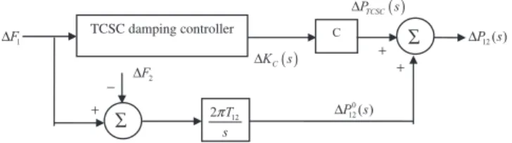
It is notable that the constant ofCcontains valuable information from the property of the TCSC device which differs it from other series FACTS such as SSSC. It is clear from Eq.(14) that the tie-line power flow exchange can be regulated continuously by dynamic control of the DKC. In order to realize an appropriate

damping controller based on the TCSC, theCconstant is included in the TCSC proportional gain. The structure of TCSC as frequency controller is shown inFig. 2, where the frequency deviation in area 1 i.e.,DF1is used as the input control signal.

5. TCSC damping controller

5.1. Phase lead-lag based TCSC damping controller

The transfer function model of the TCSC-based damping con-troller with phase lead-lag structure is considered as:

D

KCðsÞ ¼ KTCSC 1þsTTCSC 1þsT1 1þsT2 1þsT3 1þsT4

D

F1ðsÞ ð16Þ where the adjustable gain and time constant of TCSC are denoted by

KTCSCandTTCSC, respectively. In order to decrease the computational

burden, lag time constants (T2, T4) are set to a constant as T2= T4= 0.01 s.

5.2. FOPID-based TCSC damping controller

The transfer function representation of a FOPID controller is depicted inFig. 3, and can be given by:

PIk_Dl_¼K Pþ

KI

skþKDs

l _ð17Þ

whereKP, KI, KDare the proportional, integral, and differential gains;

kand

l

are fractional order operators often adjustable in the range of (0, 1). The FOPID has two extra degrees of freedom for adjusting in comparison with the IOPID and lead-lag structure. Fork= 1 and

l

= 1, the FOPID controller reduces to the classical IOPID controller. Hence, a continuous-time FOPID-based TCSC damping controller can be expressed as:

D

KCðsÞ ¼ KPþ KI skþKDs l

D

F1ðsÞ ð18Þ

5.3. Implementation of the FOPID-based TCSC damping controller

Due to the infinite dimensional characteristic of the fractional order differentiator and integrators, their simulation is a major concern. It has been demonstrated that the band-limited imple-mentation of the FOPID controller results in sufficient performance by utilizing higher order rational integer order transfer function approximation of the FOC[2]. One of the well-known and very good approximations is Oustaloup’s bound-limited frequency domain rational recursive approximation technique[21,22]. This methodology has been used in this work and most of the former papers on the application of the FOCs[2,5–8]. The higher order analog filter, which approximates the fractional order differential termsa, is given by the following expression:

Fig. 2.Structure of proposed TCSC as frequency controller.

sa_KY N K¼N sþ

x

0 K sþ

x

K ð19Þ

where the poles, zeros, and gain of the filter can be recursively eval-uated respectively as:

x

K¼

x

bð

x

h=

x

bÞ KþNþ1 2ð1þaÞ 2Nþ1 ;

x

0 K¼

x

bð

x

h=

x

bÞ KþNþ1 2ð1aÞ 2Nþ1 ;K¼

x

a h ð20Þ where

a

is the fractional order; (2N + 1) is the order of the approximation filter; and (

x

b,

x

h) is the expected fitting range or

frequency range of controller operation. Even with this approxima-tion, the obtained FOPID controller is found to outperform IOPID controller in most recent works[2,5–8]. In fact, there is a trade-off between the complication of the FOPID realization and accuracy. Efficient guidelines for evaluating the lower and upper bounds and the order of the Oustaloup approximation are studied in[22]. In this work, 5th order Oustaloup’s recursive approximation is considered within the frequency bound of

x

e

(102_,102_{) rad/s which is most} typical range in the FOPID applications[5].

A widely-employed approach for time domain simulation of systems containing non-integer order controllers is to approximate the FOC with an integer order rational transfer function and then perform the simulation [5–8]. Nowadays, the computations and simulations associated with fractional order control issues can be carried out easily using MATLAB/SIMULINK based toolboxes which are dedicated to fractional order control such as FOMCON toolbox

[23]. The FOMCON stands for fractional order modeling and control toolbox developed for MATLAB software to analysis of fractional systems and controllers in both time and frequency domains. The goal of this toolbox is to provide a user-friendly, powerful and accurate means of conducting with the FOCs for a wide range of practical applications[3,24]. The dynamic model of the case study power system has been developed in the MATLAB/SIMULINK envi-ronment. All simulations of this paper are performed using the FOMCON toolbox version 0.3-alpha (R-2012-09-20).

6. Problem formulation and optimization

6.1. Proposed objective function for optimal coordinated controller design

In order to damp the tie-line power and frequency oscillations successfully, the integral of time multiplied squared error (ITSE) performance index is considered as the objective function[15]:

ITSE¼ Z Tsim 0 t½Df21þ

D

f 2 2þ

D

P 2 12dt ð21Þ

whereTsimdenotes the simulation time. The ITSE index takes

advan-tages of both integral of squared error (ISE) and integral of time multiplied absolute error (ITAE) performance indices, as it uses squared error and time multiplication to mitigate large oscillations and reduce long settling time. The adjustable parameters of consid-ered coordinated controllers are summarized inTable 1.

The adjustable parameters of the coordinated controllers are optimized simultaneously via minimizing the ITSE index employ-ing improved particle swarm optimization (IPSO) algorithm [15]

subject to following constraints:

KminI1 6KI16KmaxI1 ;K min I2 6KI26KmaxI2 ;K min TCSC6KTCSC6KmaxTCSC; Kmin

P 6KP6KmaxP ;KminI 6KI6KmaxI ;KminD 6KD6KmaxD ; Tmin TCSC6TTCSC6TmaxTCSC;T min 1 6T16Tmax1 ;T min 3 6T36Tmax3 ;06k61;06

l

61

ð

22

Þ

where all gains and time constants are optimized in the range of (0, 2) and (0.01, 1), respectively.

6.2. IPSO algorithm

In the PSO algorithm, the particles as candidate solutions move inside a multidimensional exploration space in accordance with the velocity and position updating rules. Each particle stores its best flying position which is experienced so far in pbest. Also the

best flying position found by the swarm till now is stored asgbest.

Thepbestandgbestare updated during iterations and particles try

to enhance their positions by following the properties from their winning fellows. The velocity and position update rules in the stan-dard PSO algorithm are[25,26]:

v

ðtþ1Þ j;k ¼

x:

v

ðtÞ j;kþc1:r1:ðpbest j;kx ðtÞ j;kÞ þc2:r2:ðgbest kx ðtÞ j;kÞ ð23Þ xðtþ1Þj;k ¼x ðtÞ j;kþ

v

ðtþ1Þ j;k ; ð24Þ

wherej =1, 2,. . .,n; k =1, 2,. . .,m. Parameternis the population size;mis total number of the parameters to be optimized;

x

is iner-tia weight in interval of (0, 1) that normally is reduced in each iter-ation; and random numbers ofr1andr2follow uniform distribution in range of (0, 1). The acceleration factorsc1andc2are learning parameters called cognitive and social constants. The cognitive fac-torc1describes the trend toward following the best winning action

Fig. 3.FOPID based TCSC damping controller.

Table 1

Adjustable parameters of considered coordinated controllers.

Coordinated controller Adjustable parameters

Lead-lag based TCSC damping controller in coordination with integral AGC TTCSC, KTCSC, T1, KI1, KI2 IOPID based TCSC damping controller in coordination with integral AGC KP, KI, KD, KI1, KI2 FOPID based TCSC damping controller in coordination with integral AGC KP, KI, KD,k,l, KI1, KI2

Table 2

Optimal parameters of the coordinated controllers.

Controller type KI1 KI2 KTCSC TTCSC T1 T3 KP KI k KD l Lead-lag TCSC-AGC 0.1254 0.1858 0.1109 0.0761 0.3621 0.5978 – – – – – IOPID TCSC-AGC 0.1249 0.1686 – – – – 0.0931 0.0546 – 0.1211 – FOPID TCSC-AGC 0.1210 0.1661 – – – – 0.1335 0.0630 0.9667 0.1705 0.7079 0 5 10 15 20 25 30 35 40 45 50 -0.045 -0.04 -0.035 -0.03 -0.025 -0.02 -0.015 -0.01 -0.005 0 0.005 Time(s) A rea 1 f req u en cy d evi at io n ( H z) FOPID IOPID lead-lag (a) 0 5 10 15 20 25 30 35 40 45 50 -0.05 -0.04 -0.03 -0.02 -0.01 0 0.01 Time(s) A re a 2 fr eque nc y de v ia tio n (H z) FOPID IOPID lead-lag (b) 0 5 10 15 20 25 30 35 40 -20 -15 -10 -5 0 5x 10 -3 Time(s) T ie -lin e p o we r de v ia tio n ( p u M W ) FOPID IOPID lead-lag (c)

Fig. 4.Dynamic responses to the SLP in area 1, (a) Area 1 frequency deviationDf1, (b) Area 2 frequency deviationDf2, and (c) Tie-line power deviationDP12.

of the particle, while the social factorc2represents the tendency to track the most successful action of the flock, i.e.,c1, c2are in charge

of updating the particle velocity at the course of pbest and gbest,

respectively. Small accelerating factors make particles to wander

far from the objective region while large values cause swift movements towards the objective region or may extrude the region. There should be reasonable cooperation among three terms of the velocity updating rule to increase the capability of the PSO

Table 3

System damping characteristics obtained by employing different controllers.

0 5 10 15 20 25 30 -0.2 -0.15 -0.1 -0.05 0 0.05 0.1 0.15 0.2 Time(s) Si nus o id a l l o a d (puM W )

(a)

0 5 10 15 20 25 30 -0.1 -0.05 0 0.05 0.1 0.15 Time(s) A rea 1 f req u en cy d evi at io n ( H z) lead-lag FOPID IOPID

(b)

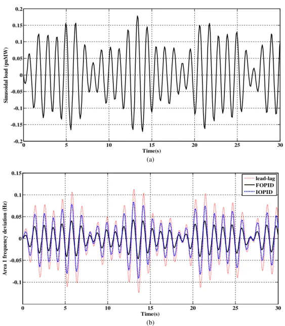
Fig. 5.Dynamic responses to the sinusoidal load perturbation in area 1, (a) Sinusoidal load perturbation, (b) Area 1 frequency deviation, (c) Area 2 frequency deviation, and (d) Tie-line power deviation.

algorithm, where the terms are called weighted, cognitive, and social parts. The termsxj,k(t),

v

j,k(t)denote thekthcomponents of the

position and velocity vectors of the particlejat iteration oft. The inertia weight and acceleration coefficients are important parame-ters for evaluating the performance of the PSO algorithm. A large inertia weight near to maximum value helps particles global explo-ration capability while a smaller one has a tendency towards local exploration. An appropriate selection of the inertia weight can result in a balance between global exploration and local exploita-tion[27]. This leads to less iteration to obtain the optimal solution. Usually, a linearly decreasing inertia weight over the iterations is considered widely in the PSO applications as:

x

ðtÞ_¼

x

max

x

max

x

min

itermax :

iterðtÞ ð25Þ

where

x

(t)_{denotes the normal inertia weight in iterationt;iter} maxis

total number of the iterations; and constants

x

max,

x

minare the

ini-tial and final inertia weights, respectively.

In order to take maximum advantage of the proposed controller, it is very important that what optimization mechanism is used to tune carefully the adjustable parameters. The standard PSO has

great advantages in comparison with similar swarm-based algo-rithms such as genetic algorithm (GA)[25]. The standard PSO can be coded simply in a few lines since it has a few algorithm param-eters while it uses an efficient optimization technique to obtain the global optimal solution[25]. Furthermore, in contrary with the GA, the PSO provides the capability of establishing a balance between global and local explorations[25]. However, the standard PSO still may have some drawbacks such as exploration problem due to the risk of trapping in local minimal as a result of premature conver-gence, exploitation problem due to the inadequate capability to explore near borderline points of the search space[27]. In order to overcome the drawbacks of the standard PSO, IPSO algorithm has been introduced recently in [27]. This version of the PSO employs a new dynamic inertia weight by combining chaotic sequences with the linearly reducing inertia weights as:

ch

x

ðtÞ_¼

x

ðtÞ

c

ðtÞ _ð26Þ

wherech

x

(t)_{is a chaotic weight at iterationtand}

c

(t)_{is the chaotic}

parameter. Since the proposed chaotic inertia weight decreases and oscillates concurrently, it can cover the whole inertia weight area under the descending line in a chaotic procedure and the exploring

0 5 10 15 20 25 30 -0.015 -0.01 -0.005 0 0.005 0.01 0.015 Time(s) A rea 2 f req u en cy d evi at io n ( H z) IOPID FOPID lead-lag

(c)

0 5 10 15 20 25 30 -0.015 -0.01 -0.005 0 0.005 0.01 0.015 Time(s) Ti e-li n e p o w er d evi at io n ( p u MW) FOPID IOPID lead-lag

(d)

Fig. 5(continued)

capability of the proposed IPSO algorithm can be enhanced effec-tively[27]. Moreover, the proposed IPSO uses a crossover operator inspired by the GA to enhance both exploration and exploitation capabilities of the standard PSO. Therefore, the search quality is improved by avoiding premature convergence via increased diver-sity of the swarm. This can help in effective exploration and exploitation of the hopeful zones in the search space to find the globally optimal solution more precisely. When the value of cross-over rate (CR) becomes one, there is no crosscross-over similar to the standard PSO. If the value of CR is zero, the position will always have the crossover operation similar to the GA[27]. An appropriate CR can be obtained by empirical examinations to increase the swarm diversity. The parameters of the IPSO algorithm should be selected carefully to provide high performance. Hence, initially some executions have been performed with different values of the IPSO parameters to assess if IPSO will find satisfactory results or not. For our provided MATLAB-based IPSO program, the algorithm parameters are chosen as n =30;

x

min=0.4;

x

max=0.9;

l

=4;

c

0=0.54; c1= c2=2; itermax= 30; and CR = 0.6, where

l

is a control

parameter and

c

0is initial chaotic parameter[27]. More details can

be found in[27]about the employed IPSO algorithm.

7. Simulation results and discussion

Prior to presenting the simulation outcomes, it seems to be use-ful to enumerate briefly what simulation procedure is going to carry out to evaluate the performance of the coordinated con-trollers. The simulation process can be arranged into following headers:

Performance evaluation under step, sinusoidal, and random load perturbation patterns.

Sensitivity analysis to assess the robustness of the coordinated controllers against ±50% uncertainty in system loading condi-tion and parameter.

7.1. Performance evaluation for step load perturbation

In this case, the dynamic responses are obtained for 0.01 p.u. step load perturbation (SLP) in area 1. The optimal parameters are listed in Table 2. Fig. 4 illustrates the area frequency and tie-line power oscillations. The ‘‘lead-lag”, ‘‘IOPID”, and ‘‘FOPID”

0 20 40 60 80 100 120 140 160 180 200 -0.005 0 0.005 0.01 0.015 0.02 0.025 0.03 0.035 0.04 0.045 Time(s) Ran d om load ( p u M W)

(a)

0 20 40 60 80 100 120 140 160 180 200 -0.1 -0.05 0 0.05 0.1 0.15 0.2 0.25 Time(s) A rea 1 f req u en cy d evi at io n ( H z) IOPID lead-lag FOPID

(b)

Fig. 6.Dynamic responses to the random step load perturbation in area 1, (a) Random step load perturbation, (b) Area 1 frequency deviation, (c) Area 2 frequency deviation, and (d) Tie-line power deviation.

legends stand for the lead-lag based TCSC-AGC, IOPID-based TCSC-AGC, and FOPID-based TCSC-AGC, respectively. It is notable that since the applied perturbation is an incremental load; the fre-quencies drop down at first with undershoots. Also, it can be observed that the coordination of the lead-lag based TCSC and integral AGC can mitigate the deviations to zero within large and long-lasting oscillations. With the application of the IOPID-based TCSC-AGC controller, the damping profiles are better than those obtained by the lead-lag based TCSC-AGC. However, the oscillatory nature of responses still remains the same. Absolutely, it is explicit that the proposed FOPID-based TCSC-AGC coordinated damping controller outperforms the IOPID and lead-lag structure in damp-ing of the area frequency and tie-line power oscillations and improving the system transient behavior in terms of decreased amplitude and settling time of the oscillations.

The damping measures such as the system oscillatory modes and corresponding damping ratios, ITSE performance index, maxi-mum peak, peak time, and settling time of the oscillations are determinant in the dynamic performance evaluations. These crite-ria are summarized inTable 3. Only the oscillatory modes obtained

after linearization of the system are listed and the negative real eigenvalues are not listed here for simplicity. The linearization technique used by MATLAB obtains linear state space models from systems of differential equations described as Simulink models. This technique uses preprogrammed analytic block Jacobians for most blocks which should result in more accurate linearization than numerical perturbation of block inputs and states[28].

It is evident from Table 3 that with proposed FOPID-based TCSC-AGC, the obtained ITSE index is the smallest value among others which shows the most promising controller. The highlighted rows ofTable 3indicate the system minimum damping ratio (fmin)

obtained by application of each controller type. It is clear that by employing the FOPID-based TCSC-AGC, fmin= 0.3693 shows an

increase of approximately two times in comparison with employ-ing of the lead-lag based TCSC-AGC (fmin=0.1706). Furthermore,

by employing the FOPID-based TCSC-AGC, the settling time and maximum peak of the oscillations have been decreased.

FromFig. 4andTable 3, it is evident that the damping charac-teristics obtained by employing the FOPID-based TCSC-AGC are remarkably better than those of obtained by the lead-lag and IOPID

0 20 40 60 80 100 120 140 160 180 200 -0.2 -0.15 -0.1 -0.05 0 0.05 0.1 0.15 0.2 0.25 Time(s) A rea 2 f req u en cy d evi at io n ( H z) IOPID FOPID lead-lag

(c)

0 20 40 60 80 100 120 140 160 180 200 -0.05 -0.04 -0.03 -0.02 -0.01 0 0.01 0.02 0.03 0.04 0.05 Time(s) T ie -l ine pow er de vi at io n (puM W) IOPID lead-lag FOPID

(d)

Fig. 6(continued)

0 10 20 30 40 50 60 70 80 90 100 -0.25 -0.2 -0.15 -0.1 -0.05 0 0.05 Time(s) A rea 1 f req u en cy d evi at io n ( H z) lead-lag FOPID IOPID

(a)

0 10 20 30 40 50 60 70 80 90 100 -0.25 -0.2 -0.15 -0.1 -0.05 0 0.05 Time(s) Area 2 f req u en cy d evi at io n ( H z) lead-lag FOPID IOPID

(b)

0 10 20 30 40 50 60 70 80 90 100 -0.1 -0.08 -0.06 -0.04 -0.02 0 0.02 0.04 0.06 0.08 0.1 Time(s) T ie -l ine pow er de vi at io n (puM W) lead-lag FOPID IOPID

(c)

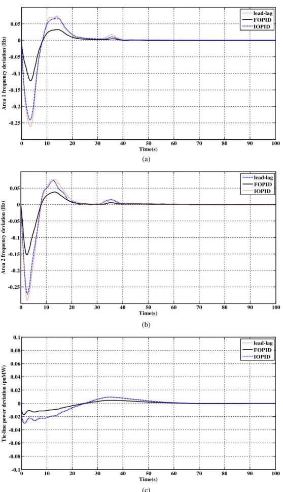
Fig. 7.Dynamic responses to the higher value of step load perturbation in area 1, (a) Area 1 frequency deviation, (b) Area 2 frequency deviation, and (c) Tie-line power deviation.

cases. Hence, for the SLP, the frequency stability is enhanced out-standingly by using the FOPID-based TCSC in coordination with the integral AGC.

7.2. Performance evaluation for sinusoidal load perturbation

In order to evaluate the effectiveness of considered controllers in stabilization of the area frequency and tie-line power oscillations under continuous load pattern, the sinusoidal load per-turbation is applied in area 1 as following[11,19]:

D

Pd1¼0:03 sinð4:36tÞ þ0:05 sinð5:3tÞ 0:1 sinð6tÞ ð27Þ

Fig. 5depicts the considered sinusoidal load perturbation and the corresponding dynamic responses. The illustrations reveal that the area frequency and tie-line power oscillations are restricted most effectively using the FOPID-based TCSC-AGC. As seen in

Fig. 5, in contrast to the previous perturbation patterns, only the amplitude of oscillations is limited which means that the oscilla-tions are not damped out entirely due to the nature of the sinu-soidal waveform. However, the FOPID-based TCSC-AGC controller provides the greatest stabilizing performance to the oscillations in comparison to the others.

7.3. Performance evaluation for random load perturbation

In this case, a random step load perturbation as depicted inFig. 6 [29]is applied in area 1. The steps are random both in magnitude and duration in accordance with the nature of load changes in a real-istic power system. The dynamic responses of the interconnected power system under the random perturbation are shown inFig. 6. It is obvious fromFig. 6that the proposed controller provides great damping even in the presence of random step load perturbation.

7.4. Performance evaluation for higher degree of step load perturbation

A further case study is added to demonstrate the superiority of the proposed controller when subjected to a higher degree of step load disturbance[30]. In this scenario, the dynamic responses are obtained for 0.05 p.u. SLP in area 1. The same controller parameters obtained before are employed in this part. It can be observed from the illustrated results inFig. 7, that the proposed controller pro-vides much greater dynamic performance than the other con-trollers even when the magnitude of the SLP is extended from 0.01 p.u. to 0.05 p.u.

Table 4

Sensitivity analysis for wide range of loading condition and system parametric uncertainty.

0 5 10 15 20 25 30 35 40 45 50 -0.035 -0.03 -0.025 -0.02 -0.015 -0.01 -0.005 0 0.005 0.01 Time(s) A rea 1 f req u en cy d evi at io n ( H z) nominal loading +50% of nominal loading -50% of nominal loading

(a)

0 5 10 15 20 25 30 35 40 45 50 -0.05 -0.04 -0.03 -0.02 -0.01 0 0.01 Time(s) A rea 2 f req u en cy d evi at io n ( H z) nominal loading +50% of nominal loading -50% of nominal loading

(b)

0 5 10 15 20 25 30 35 40 -0.02 -0.015 -0.01 -0.005 0 0.005 Time(s) T ie -l ine po w er de v ia ti o n (puM W ) nominal loading +50% of nominal loading -50% of nominal loading

(c)

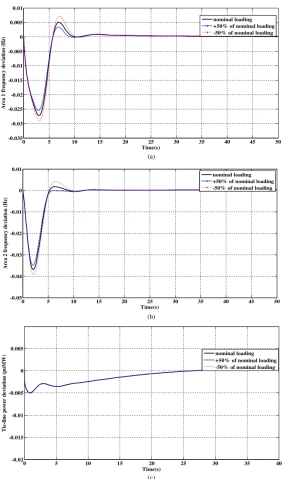
Fig. 8.Dynamic responses of the system equipped with the proposed controller under the uncertainties in loading condition.

0 5 10 15 20 25 30 35 40 45 50 -0.035 -0.03 -0.025 -0.02 -0.015 -0.01 -0.005 0 0.005 0.01 Time(s) A rea 1 f req u en cy d evi at io n ( H z) nominal T12 +50% of nominal T12 -50% of nominal T12

(a)

0 5 10 15 20 25 30 35 40 45 50 -0.05 -0.04 -0.03 -0.02 -0.01 0 0.01 Time(s) A rea 2 f req u en cy d evi at io n ( H z) nominal T12 +50% of nominal T12 -50% of nominal T12

(b)

0 5 10 15 20 25 30 35 40 -20 -15 -10 -5 0 5x 10 -3 Time(s) T ie-li n e p o w er d evi at io n ( p u MW) nominal T12 +50% of nominal T12 -50% of nominal T12

(c)

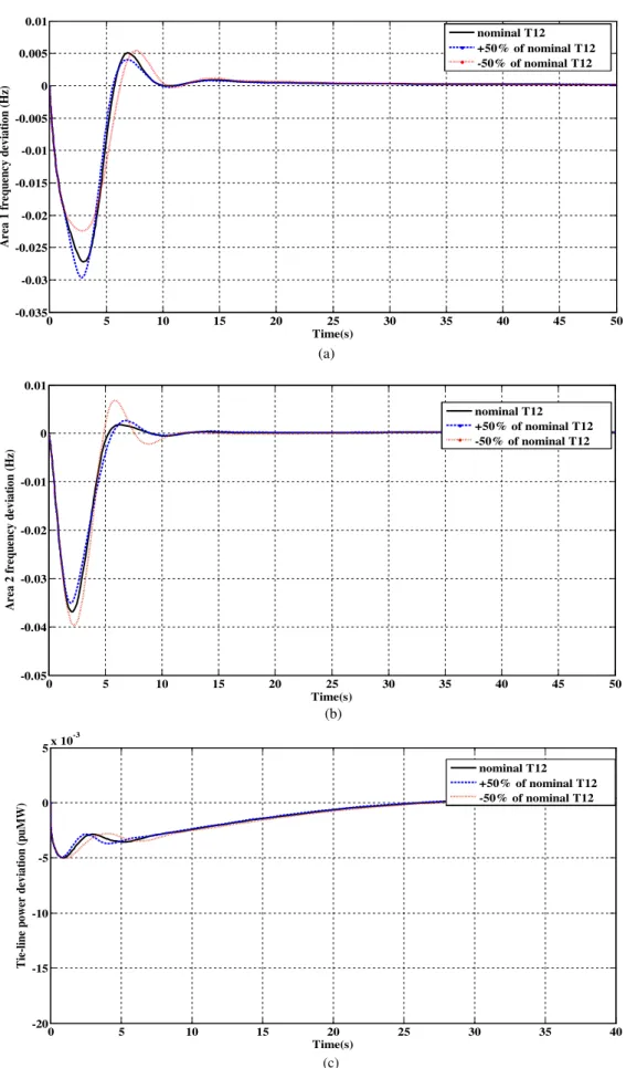
Fig. 9.Dynamic responses of the system equipped with the proposed controller under the uncertainties in synchronizing coefficient (T12).

7.5. Sensitivity analysis

In order to evaluate the robustness of the power system under large changes in the system loading condition and parameters,

sen-sitivity analyses are performed. The system loading condition and the synchronizing coefficient are chosen as two most affecting parameters of the AGC performance to apply the large changes. In doing so, these parameters are varied by ±50% of nominal values,

0 5 10 15 20 25 30 35 40 45 50 -0.04 -0.03 -0.02 -0.01 0 0.01 Time(s) Area 1 f req u en cy d evi at io n ( H z) IPSO Standard PSO Standard GA

(a)

0 5 10 15 20 25 30 35 40 45 50 -0.05 -0.04 -0.03 -0.02 -0.01 0 0.01 Time(s) A rea 2 f req u en cy d evi at io n ( H z) IPSO Standard PSO Standard GA

(b)

0 5 10 15 20 25 30 35 40 -20 -15 -10 -5 0 5x 10 -3 Time(s) Ti e-li n e p o w er d evi at io n ( p u M W) IPSO Standard PSO Standard GA

(c)

Fig. 10.Standard PSO and GA versus IPSO, (a) Area 1 frequency deviation, (b) Area 2 frequency deviation, and (c) Tie-line power deviation.

independently and the results for the 0.01 p.u. SLP in area 1 are presented inTable 4for the simulation time of 50 s. As we know, the Increase/decrease in the ITSE index can be interpreted as decline/improvement of the system frequency stability. Also, the smaller damping ratios mean the deteriorative damping behavior. It can be noticed fromTable 4that by applying ±50% uncertainties in the loading condition and synchronizing coefficient, the values of the ITSE index, system oscillatory modes, corresponding damp-ing ratios, maximum peaks, peak times, and settldamp-ing times of the oscillations deviate from their nominal values somewhat. How-ever, it can be noticed that by applying the ±50% drastic changes, the power system is still dynamically stable since the damping measures are near to the nominal values and the area frequency and tie-line power oscillations settle within maximum 30 s. For better insight into the results of sensitivity analyses, the area frequency and tie-line power oscillations under the considered uncertainty scenarios are presented in Figs. 8 and 9. It can be observed from these illustrations that in the case of employing FOPID-based TCSC-AGC, the large and imposing uncertainties (±50%) have negligible impact on the system overall dynamic per-formance. Briefly, the sensitivity analyses demonstrate that the system equipped with the FOPID-based TCSC-AGC is meaningfully robust to the considered variations. As a result, once the adjustable parameters of the proposed controller are optimized in nominal condition, there is no need to reset for the ±50% changes in the syn-chronizing coefficient and loading condition.

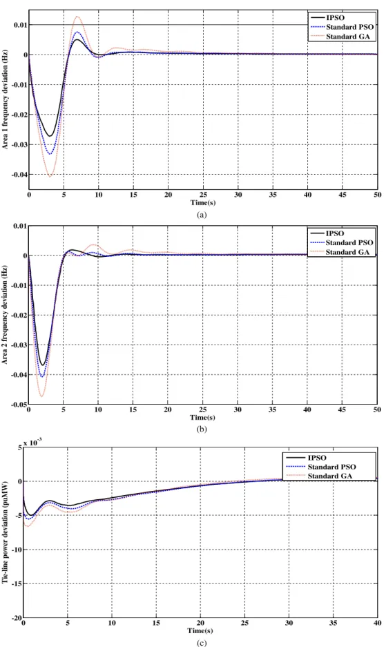
7.6. IPSO in comparison with standard PSO and GA

For the sake of comparison with the IPSO, the standard PSO and GA are also used to optimize the adjustable parameters of the TCSC-AGC coordinated controller. The parameters of the standard PSO are chosen as: n =30; m = 7;

x

min=0.4;

x

max=0.9; c1= c2=2; itermax= 30. The optimized parameters obtained by the

standard PSO are KI1=0.1189; KI2=0.1710; KP=0.1423; KI=0.0660;k=0.8452;KD= 0.2659;

l

=0.8750 with ITSE = 0.0193

andfmin= 0.2984. The optimized parameters obtained by the

stan-dard GA are KI1=0.1424; KI2=0.1534; KP=0.1279; KI=0.0619;

k=0.8990; KD= 0.3190;

l

=0.9011with ITSE = 0.0204 and

fmin= 0.2613. It can be seen that by employing the standard PSO

and GA, the ITSE index is increased and the minimum damping ratio is decreased in comparison with the results obtained by using the IPSO algorithm. This means that when the IPSO is used to adjust the controller, the system damping characteristics are the highest in comparison with using the standard PSO and GA.

Fig. 10shows the frequencies and tie-line power oscillations for 0.01 p.u. SLP in area 1. It is obvious fromFig. 10that when the IPSO is used to optimize the adjustable parameters, the obtained dynamic responses are the best. In a lower level, the standard PSO algorithm outperforms the standard GA to provide better results.

8. Conclusion

In this paper, a new application for the FOC as the FACTS-based damping controller has been investigated. The FOPID has been applied in the design of the TCSC-based damping controller to improve the AGC performance of the interconnected multi-source power system. The physical constraints of the GRC nonlin-earity and GDB effect are also taken into account for a challenging realization. In doing so, the contribution of the TCSC in the tie-line power exchange has been formulated analytically. Then, the strategy of the coordinated control of the proposed FOPID-based TCSC damping controller and the AGC loop has been proposed. The IPSO algorithm which is reinforced by chaotic parameter and

crossover operator has been used to obtain the global optimal solu-tion. The dynamic performance of the proposed controller is com-pared with the PID and phase lead-lag based counterparts under the step, sinusoidal and random load perturbation patterns. The simulations reveal that the proposed controller provides the high-est dynamic performance in comparison with the other controllers in terms of increased minimum damping ratio, decreased ITSE, decreased maximum peak and settling time of the area frequency and tie-line power oscillations. Furthermore, the carried out sensitivity analyses show that the power system equipped with the proposed controller is meaningfully robust to the considered large uncertainty scenarios.

References

[1]C.A. Monje, B.M. Vinagre, V. Feliu, Y. Chen, Tuning and auto-tuning of fractional order controllers for industry applications, Control Eng. Pract. 16 (7) (2008) 798–812.

[2]D. Valério, J. da Costa, Introduction to single-input, single-output fractional control, IET Control Theory Appl. 5 (8) (2011) 1033–1057.

[3]A. Tepljakov, Fractional-order Calculus based Identification and Control of Linear Dynamic Systems MSc thesis, Faculty of Information Technology, Department of Computer Control, Tallinn University of Technology, Tallinn, Estonia, 2011.

[4]S. Debbarma, L.C. Saikia, N. Sinha, AGC of a multi-area thermal system under deregulated environment using a non-integer controller, Electr. Pow Syst. Res. 95 (2013) 175–183.

[5]I. Pan, S. Das, Chaotic multi-objective optimization based design of fractional order PIk_Dl_{controller in AVR system, Int. J. Electr. Power 43 (1) (2012) 393–}

407.

[6]M. Zamani, M. Karimi-Ghartemani, N. Sadati, M. Parniani, Design of a fractional order PID controller for an AVR using particle swarm optimization, Control Eng. Pract. 17 (12) (2009) 1380–1387.

[7]I. Pan, S. Das, Frequency domain design of fractional order PID controller for AVR system using chaotic multi-objective optimization, Int. J. Electr. Power 51 (2013) 106–118.

[8]Y. Tang, M. Cui, C. Hua, L. Li, Y. Yang, Optimum design of fractional order PIkDl controller for AVR system using chaotic ant swarm, Expert Syst. Appl. 39 (8) (2012) 6887–6896.

[9]C.K. Shiva, V. Mukherjee, A novel quasi-oppositional harmony search algorithm for AGC optimization of three-area multi-unit power system after deregulation, Eng. Sci. Technol., Int. J. 19 (1) (2016) 395–420.

[10]R.K. Sahu, T.S. Gorripotu, S. Panda, Automatic generation control of multi-area power systems with diverse energy sources using teaching learning based optimization algorithm, Eng. Sci. Technol., Int. J. 19 (1) (2016) 113–134.

[11]P.C. Pradhan, R.K. Sahu, S. Panda, Firefly algorithm optimized fuzzy PID controller for AGC of multi-area multi-source power systems with UPFC and SMES, Eng. Sci. Technol., Int. J. 19 (1) (2016) 338–354.

[12]M.I. Alomoush, Load frequency control and automatic generation control using fractional-order controllers, Electr. Eng. 91 (7) (2010) 357–368.

[13]I. Chathoth, S.K. Ramdas, S.T. Krishnan, Fractional-order proportional-integral-derivative-based automatic generation control in deregulated power systems, Electr. Pow Compo. Syst. 43 (17) (2015) 1931–1945.

[14]T.S. Gorripotu, R.K. Sahu, S. Panda, AGC of a multi-area power system under deregulated environment using redox flow batteries and interline power flow controller, Eng. Sci. Technol. Int. J. (2015).

[15]K. Zare, M.T. Hagh, J. Morsali, Effective oscillation damping of an interconnected multi-source power system with automatic generation control and TCSC, Int. J. Electr. Power 65 (2015) 220–230.

[16]J. Morsali, K. Zare, M.T. Hagh, Performance comparison of TCSC with TCPS and SSSC controllers in AGC of realistic interconnected multi-source power system, Ain Shams Eng. J. (2015).

[17]S. Padhan, R.K. Sahu, S. Panda, Automatic generation control with thyristor controlled series compensator including superconducting magnetic energy storage units, Ain Shams Eng. J. 5 (3) (2014) 759–774.

[18]M. Deepak, R.J. Abraham, Load following in a deregulated power system with thyristor controlled series compensator, Int. J. Electr. Power Energy Syst. 65 (2015) 136–145.

[19]P. Bhatt, R. Roy, S. Ghoshal, Comparative performance evaluation of SMES– SMES, TCPS–SMES and SSSC–SMES controllers in automatic generation control for a two-area hydro–hydro system, Int. J. Electr. Power Energy Syst. 33 (10) (2011) 1585–1597.

[20]J. Morsali, k. Zare, M.T. Hagh, AGC of Interconnected Multi-source Power System with Considering GDB and GRC Nonlinearity Effects, 6th Conference on Thermal Power Plants (Gas, Combined-Cycle, Steam), IEEE, Iran University of Science and Technology, Tehran, Iran, 2016. 19–20 January.

[21]A. Oustaloup, F. Levron, B. Mathieu, F.M. Nanot, Frequency-band complex noninteger differentiator: characterization and synthesis, IEEE T Circuits-I 47 (1) (2000) 25–39.

[22]F. Merrikh-Bayat, Rules for selecting the parameters of Oustaloup recursive approximation for the simulation of linear feedback systems containing PIk_Dl

controller, Commun. Nonlinear Sci. 17 (4) (2012) 1852–1861.

[23]A. Tepljakov, E. Petlenkov, J. Belikov, FOMCON: a MATLAB Toolbox for Fractional-order System Identification and Control, Int. J. Microelectron. Comput. Sci. 2 (2) (2011) 51–62.

[24]A. Tepljakov, E. Petlenkov, J. Belikov, S. Astapov, Tuning and digital implementation of a fractional-order PD controller for a position servo, Int. J. Microelectron. Comput. Sci. 4 (3) (2013) 116–123.

[25]B.K. Panigrahi, A. Abraham, S.E. Das, Computational intelligence in power engineering, Springer-Verlag, Berlin Heidelberg, 2010.

[26]J. Kennedy, R.C. Eberhart, Swarm intelligence, Morgan Kaufmann, San Francisco, 2001.

[27]J.-B. Park, Y.-W. Jeong, J.-R. Shin, K.Y. Lee, An improved particle swarm optimization for nonconvex economic dispatch problems, IEEE T Power Syst. 25 (1) (2010) 156–166.

[28] MATLAB Manual, MATLAB: The language of technical computing, The MathWorks, Inc.http://www.mathworks.com,2012.

[29]M. Shiroei, M.R. Toulabi, A.M. Ranjbar, Robust multivariable predictive based load frequency control considering generation rate constraint, Int. J. Electr. Power Energy Syst. 46 (2013) 405–413.

[30] S. Debbarma, L.C. Saikia, N. Sinha, Automatic generation control using two degree of freedom fractional order PID controller, Int. J. Electr. Power 58 (2014) 120–129.