The economics of payment card fee structure: what drives payment card rewards?

The Economics of Payment

Card Fee Structures: What

Drives Payment Card

Rewards?

Fumiko Hayashi

November 2008; Revised March 2009

RWP 08-07

THE ECONOMICS OF PAYMENT CARD FEE STRUCTURE:

WHAT DRIVES PAYMENT CARD REWARDS?

Fumiko Hayashi1

First version: November 2008 This version: March 2009

RWP 08-07

Abstract: This paper investigates potential market forces that cause payment card rewards even when providing payment card rewards is not the most efficient. Three factors—oligopolistic merchants, output-maximizing card networks, and the merchant’s

inability to set different prices across payment methods—may potentially explain the prevalence of payment card rewards programs in the United States today. The paper also points out that competition among card networks may potentially make payment rewards too generous, and thus deteriorate social welfare and its distribution. The situation may potentially warrant public policy interventions.

Keywords: Payment card rewards, equilibrium fee structure, oligopolistic merchants, card network competition, no-surcharge-rules

JEL Classification: L13, L22

1

Payments System Research Function, Economic Research Department, Federal Reserve Bank of Kansas City. E-mail:fumiko.hayashi@kc.frb.org. The views expressed in this article are those of the author and do not necessarily reflect those of the Federal Reserve Bank of Kansas City or the Federal Reserve System.

1. Introduction

Payment card rewards programs have become increasingly popular in the United States.

However, providing payment card rewards may not be necessarily beneficial to consumers and

society as a whole. According to the theoretical literature on payment card fee structure, in most

cases the most efficient cardholder fees would be the difference between the card network’s costs

for a card transaction and the merchant’s transactional benefit from the card transaction.

Available empirical evidence suggests that in the United States the merchant’s transactional

benefit from a card transaction may not exceed the card network’s cost. This implies providing

rewards would unlikely be the most efficient. What drives payment card rewards?

This paper is the second of a series of three papers. The first paper examined the optimal

balance between the merchant fee and the cardholder fee from both efficiency and equity

perspectives.2

The equilibrium card fee structure is greatly influenced by many factors. This paper

examines the equilibrium fee structure under various combinations of assumptions and identifies

what factors potentially cause payment card rewards. We also consider the welfare consequences

of equilibrium card fee structures. The results suggest three factors that together may explain the

prevalence of rewards card programs in the United States today. They are oligopolistic

merchants, output-maximizing card networks and the merchant’s inability to set different prices

according to their customers’ payment methods. Whether per transaction costs and fees are fixed In this paper, we investigate what market forces drive payment card rewards. The

results are useful for policymakers when determining whether the current situation should call

for public policy interventions and if so what policies are appropriate. Policy options are

considered in the third paper.

or proportional to the transaction value may also play an important role in determining the level

of rewards. When per transaction costs and fees are proportional and the three factors mentioned

above co-exist, competition among card networks would likely increase the level of rewards as

well as the merchant fees. The higher merchant fees would result in the higher product prices,

and as a result the equilibrium social welfare would be potentially lower than the social welfare

without cards at all. Although the previous studies suggested competition in a two-sided market

may not necessarily improve efficiency, the finding in this paper—competition in a two-sided

market may potentially deteriorate efficiency—is new in the literature and has a potentially

important public policy implication.

The rest of the paper is organized as follows. Section 2 constructs theoretical models.

Section 3 examines the market equilibrium—fee structures and their welfare consequences for

different parties that are involved in payment card markets. Section 4 concludes.

2. Models

We use the models that were constructed in the first paper (Hayashi, 2008) as the base

models here. We also make additional assumptions regarding merchants and card networks,

which greatly affect equilibrium fee structure. This section first recaps our base models then

makes additional assumptions regarding merchants and card networks.

2.1Recap of the Base Models

The assumptions common to all models are the following. The payment card markets are

considered to be matured. All consumers hold at least one card and merchants accept cards as

long as the merchant fees are lower than a certain threshold level, which is endogenously

Consumers are heterogeneous in their transactional benefit from cards as opposed to the

alternative payments. A consumer’s transactional benefit from a card, b_B, consists of three parts.

One is a gross benefit minus gross cost from using a card, BBC;

3

A B

B

one is a gross benefit minus

gross cost from using the alternative payment method, ;4

A

f

and one is the consumer fee paid for

the alternative payment method, . Thus, the transactional benefit from a card is defined as:

A A B C B B B B f

b = − + . To simplify the model, we assume every consumer receives the same level of A

B

B , which is equal to A

f (i.e., A A

B f

B = ). b_B is assumed to be distributed over the interval ]

,

[b_B b_B with a density function of h(b_B), and a cumulative distribution function of H(b_B).

Consumers pay the cardholder fee of f when they use a card.

Merchants are homogeneous (at least ex-ante) and their transactional benefit from cards,

S

bˆ , is defined as the merchant cost for the alternative payment method, cSA, plus the merchant

fee paid for the alternative payment method, mA , minus the merchant cost for a card transaction,

C S

c (i.e., bˆ_S =c_SA +mA −c_SC). To simplify the model, we assume c_SC =0. Merchants pay the

merchant fee of mwhen their customers use a card. Merchants also incur a cost of selling one

unit of goods, d.

The assumptions in terms of (i) per transaction costs and fees; (ii) consumer demand for

goods; and (iii) merchant ability to set different prices according to the payment method can

vary. Per transaction costs and fees are either flat or proportional to the transaction value.

Consumer demand for goods is either inelastic (i.e., a consumer makes a fixed number of

transactions) or downward-sloping (i.e., the number of transactions increases as the effective

3

Note that gross cost does not include the fees for using a card.

price of goods decreases). A merchant either sets the same price for all of its customers

regardless of the payment method or sets the different prices according to the payment method

its customers use.

2.2Additional Assumptions

Thus, oligopolistic merchants are more realistic. This paper assumes ologopolistic

merchants compete according to the Hotelling model. Although the other models, such as the

Cournot model, can be used to describe oligopolistic merchants, the Hotelling model is more

flexible. Merchants

Although some merchants are possibly monopolistic, many U.S. merchants are

considered to be quite competitive. However, a perfectly competitive market described as the

Bertrand competition unlikely reflects the reality. At equilibrium under the Bertrand

competition, two types of merchants—cash-only merchants and card-accepting merchants—

serve the customers separately, and because of the higher price set by card-accepting merchants,

only card-using consumers make transactions at the card-accepting merchants. In reality,

however, most card-accepting merchants serve both card-using customers and non-card-using

consumers.

5

The basic framework of the Hotelling model is the following: There are two merchants,

Merchant A and Merchant B. Consumers are uniformly distributed on the interval of [0, 1],

which is independent of their transactional benefit from cards. Merchant A is located at point 0

and Merchant B is located at point 1. For the consumers located at point

x, where 0≤x≤1, the transportation cost to Merchant A is tx, and the transportation cost to Merchant B is t(1−x). A

5

For example, the Cournot model requires downward-sloping consumer demand for goods to obtain equilibrium price.

consumer located at point x with transactional benefit from cards bB chooses a merchant and a

payment method, which gives the consumer the lower effective price plus transportation costs.

For example, suppose a monopoly card network provides the card services, only Merchant A

accepts the cards, and Merchant A sets an identical pricepA for both card-using consumers and

non-card-using consumers. Merchant B sets price pB for their customers. Then, the consumer’s

effective price plus transportation cost is p_A + f −b_B +tx, when he purchases goods at Merchant A with a card, p_A +tx, when he purchases goods at Merchant A with an alternative payment method, and p_B +t(1−x), when he purchases goods at Merchant B. Suppose b_B ≥ f . The

consumer chooses a card at Merchant A, and therefore, he compares pA + f −bB +tx and

) 1

( x

t

p_B + − . If p_A + f −b_B +tx> p_B +t(1−x), then he purchases goods at Merchant B with an alternative payment method, otherwise he purchases goods at Merchant A with a card.

This paper assumes the card network sets both cardholder fees (rewards) and merchant

fees. Although, in reality, four-party scheme card networks do not directly set merchant fees,

assuming a card network sets its merchant fees is not too far from the reality because a major

part of the merchant fee (70-80 percent) is an interchange fee, almost all acquirers entirely pass

through the interchange fee to merchants, and the acquirers’ charges to merchants in addition to

the interchange fees seem not to vary very much within an industry. In contrast, assuming a card

network (four-party scheme) sets its cardholder fees may appear to be unrealistic. Cardholder

fees, especially credit card rewards, vary by card issuers: Large card issuers tend to provide more

generous rewards than their smaller counterparts. However, about 80 percent of the total

four-party scheme credit cards are issued by the top 10 card issuers. Although it is difficult to Card networks

compare the level of rewards among the top 10 issuers, if, as card networks and their issuers

claim, they compete vigorously in the consumer-side of the payment card market, then the level

of rewards should be very close to the difference between the interchange fees and the issuer’s

costs of processing a card transaction. Again, card issuers’ costs of processing a card transaction

vary. But if the top 10 issuers’ costs of processing a card transaction are similar, then the

interchange fees set by a card network greatly influence the level of rewards on the cards issued

by the top 10 issuers.

There is a variety of assumptions about the objective of payment card networks, but the

objective can be abstracted as either profit- or output-maximization. Profit-maximization is

obvious, but output-maximization may not be. When card networks compete, each card network

may reduce its markup to undercut its’ rival card networks until the markup reaches the

reservation markup. And the reservation markup may potentially be very close to zero. In such a

case, card networks likely aim to increase their market share as much as possible. Even when

card networks are monopolistic (potentially collude), their objective can be output-maximization.

In a four-party scheme card network, it is possible that each acquirer and issuer gets a small fixed

markup. Typically, an acquirer’s markup is small, and because of the intensified competition

among issuers, each issuer may get a small markup even when the card network they join is

monopolistic.

Competitive card networks’ behavior is likely affected by their cardholders’ homing

behavior. When a cardholder holds only a single-branded card or has a strong preference among

cards (singlehoming), then each card network can set monopolistic merchant fees. In contrast, if

all cardholders hold multiple cards and they are indifferent among those cards (multihoming),

their customers’ choice of payment methods. In the model, we assume that singlehoming

cardholders are not sensitive to rewards when deciding which card to use, while multihoming

cardholders are very sensitive to rewards and they always choose a card with the highest level of

rewards among the cards the merchant accepts.

In this paper, three types of card networks are considered: (i) profit-maximizing

monopoly, (ii) output-maximizing monopoly, and (iii) output-maximizing competing networks

with cardholders who are all multihoming. Although we do not explicitly consider the case of

output-maximizing competing networks with some singlehoming cardholders, the results would

be somewhere between those of an maximizing monopoly network and those of

output-maximizing duopoly networks with cardholders who are all multihoming.6

3. Market Equilibrium

Hayashi (2008) examined the most efficient fee structure under various combinations of the

assumptions. In most cases, the most efficient cardholder fee is the difference between the card

network’s costs for a payment card transaction and the merchant transactional benefit from the

card transaction. This implies that unless the merchant transactional benefit from a card exceeds

the card network’s costs of processing a card transaction, providing payment card rewards to

consumers is less efficient. According to the available cost studies in the United States, the

merchant transactional benefit from a card may not be higher than the card network’s costs.7

This section examines the equilibrium fee structures and their influence on the welfare of

different parties, such as card-using consumers, non-card-using consumers, merchants, and Nevertheless, payment card rewards programs are prevalent in the United States.

6 _{Output-maximizing networks may have a positive reservation markup per transaction; however, this section}

assumes the markup is zero (i.e., the profit of output-maximizing network is zero) for simplicity.

7

These cost studies are Garcia-Swartz et. al. (2006), Food Marketing Institute (1998), and Star Network (2006, 2007). See also Hayashi (2008) for more detailed discussion.

payment card networks (and their member financial institutions). The main purpose of this

exercise is to find out what market forces may potentially drive payment card rewards. The

results may also be useful for public policy consideration: For example, does encouraging

competition among card networks reduce the level of payment card rewards? Does regulatory

intervention that abolishes the no-surcharge rules improve social welfare?

This section looks at four factors that may significantly affect the equilibrium fee

structures. The first factor is competition among card networks and their objectives. As

mentioned above three types of card networks are considered.

The second factor is consumer demand for goods. Consumer demand for goods is assumed

to be either inelastic or downward-sloping. When a consumer’s demand for good is inelastic, the

consumer would make a fixed number of transactions regardless of the price of goods or fees

charged for each transaction. When a consumer’s demand for goods increases as the effective

price of goods (i.e., sum of the price of goods and the cardholder fee per transaction) decreases,

the consumer would make more transactions as the effective price of goods decreases.

The third factor relates to per transaction costs and fees for given payment methods. Per

transaction costs and fees are assumed to be either fixed regardless of the transaction value or

proportional to the transaction value. Many previous studies assumed that per transaction costs

and fees are fixed. In reality, however, especially in the United States, merchants pay

proportional fees for card transactions and consumers receive rewards that are proportional to the

purchase value. According to the available cost studies, costs of handling a cash transaction and

a credit card transaction increase as the transaction value increases.

Finally, the fourth factor is about the merchant’s ability to set different prices according to

price for all of their customers regardless of their payment methods. But in the other countries,

such as Australia and Netherlands, many merchants set different prices according to their

customers’ payment methods. The difference between these countries and the United States is

caused by card networks’ rules. In the United States, major card networks have a rule that does

not allow merchants to (or makes merchants difficult) set different prices according to payment

methods, while in Australia or Netherlands they do not. Especially in Australia, the Reserve

Bank of Australia prohibits the card networks from imposing such a rule.

This section first considers the case where merchants set the same price for all of their

customers regardless of their payment methods (no-discriminatory pricing). There are four

possible scenarios depending on the assumptions regarding consumer demand and per

transaction costs and fees. The first scenario is where consumer demand is fixed and per

transaction costs and fees are fixed (Scenario I). The second scenario is where consumer demand

is fixed but per transaction costs and fees are proportional to the transaction value (Scenario II).

The third scenario is where a consumer demand function is downward-sloping and per

transaction costs and fees are fixed (Scenario III). And the fourth scenario is where a consumer

demand function is downward-sloping and per transaction costs and fees are proportional to the

transaction value (Scenario IV). Except for Scenario I, analytical solutions for equilibrium fee

structure cannot be obtained. For Scenarios II and III, numerical examples can be used to

characterize the equilibrium fee structure. Therefore, this section only considers Scenarios I, II

and III. In each scenario, three types of card networks—(i) profit-maximizing monopoly, (ii)

output-maximizing monopoly, and (iii) output-maximizing competing networks with cardholders

This section then considers the case where merchants set the different prices according to

their customers’ payment methods (discriminatory pricing). Similar to the case of

non-discriminatory pricing, analytical solution is obtainable only for Scenario I. Numerical examples

can be used for Scenario II. Thus, only two scenarios are considered in this case.

Because tedious calculations are required to obtain market equilibrium fee structures under

various combinations of assumptions, the below summarizes the results. Detailed calculations

are in the Appendix.

3.1 Market Equilibrium under No-discriminatory Pricing

Tables 1 and 2 summarize the equilibrium fee structure and the welfare consequences,

respectively, when merchants set the same price for card-using consumers and consumers who

use an alternative payment method. There are several key observations.

First, in all three scenarios, a profit-maximizing monopoly network would set the most

efficient cardholder fees. This implies that if providing rewards to card-using consumers is not

the most efficient, then the profit-maximizing monopoly network would not provide rewards.

However, this does not necessarily imply that social welfare is maximized under a

profit-maximizing card network. Except for Scenario I, social welfare is also affected by the product

price, which is affected by the merchant fee. The merchant fee set by the profit-maximizing

monopoly network is higher than the merchant’s transactional benefit from cards, which implies

the merchant fee is not necessarily at the most efficient level. As a result, with profit-maximizing

monopoly network(s), social welfare may not be reached at the maximum level (except for

Scenario I).

Second, in all three scenarios, an output-maximizing monopoly network would set

providing rewards is not the most efficient, the output-maximizing monopoly network would

likely provide rewards to card-using consumers. Because the highest merchant fee the monopoly

network can set increases as the cardholder fee decreases (or the level of rewards increases), the

merchant fee set by the output-maximizing monopoly network is higher than that set by the

profit-maximizing monopoly network. As a result, the equilibrium product prices set under the

output-maximizing monopoly network are higher than those set under the profit-maximizing

monopoly network. Social welfare under the output-maximizing monopoly network is also lower

than that under the profit-maximizing monopoly network.

Third, whether competing card networks would set their cardholder fees at the most

efficient level depends on two factors. One is cardholders’ homing behavior and the other is the

nature of per transaction costs and fees. When all cardholders are singlehoming (either they have

only one card or they have a strong preference and cardholder fees do not affect their card

choice), competing card networks can act like an output-maximizing monopoly network. When

all cardholders are multihoming (i.e., they have multiple networks’ cards and are indifferent

among cards as long as the cardholder fees are the same), the equilibrium cardholder fee depends

on whether per transaction costs and fees are fixed (Scenario I) or proportional to the transaction

value (Scenario II). If the former is the case, the competing card networks would set their

cardholder fee at the most efficient level and their merchant fee at the merchant’s transactional

benefit. This is because oligopolistically competing merchants would only accept the cards with

the lower merchant fee. If the latter is the case, the competing card networks would set their

cardholder fees as low as possible. As a result, the merchant fees can be higher than the fees set

by monopoly card networks. In this case, two types of merchants would co-exist ex-post: One

of merchants would accept both networks’ cards. In fact, the card network with the higher

merchant fee (thus the lower cardholder fees) would have more transactions than its rival card

network. Knowing at least some merchants would accept both cards, card networks would not

lower their merchant fees. Rather, they would raise merchant fees and lower cardholder fees in

order to increase their card transactions.8

8

The card network can increase its merchant fee until one type of merchants would become more profitable by rejecting both cards than rejecting the cards with the higher merchant fees, given the other type of merchants would accept both networks’ cards.

Thus, competition among card networks would likely

increase the equilibrium merchant fee and the level of payment card rewards.

Fourth, related to the previous observations, whether per transaction costs and fees are

fixed (Scenario I and III) or proportional to the transaction value (Scenario II) would

significantly affect social welfare. If the former is the case, social welfare with cards is always at

least the same as social welfare without cards. While merchant profits are not affected by

competition among card networks and their objectives, the surplus of consumers as a whole is

higher when card networks are competing (Scenario I). In contrast, if the latter is the case

(Scenario II), social welfare with cards is not always higher than or the same as social welfare

without cards. Social welfare under profit-maximizing monopoly network is always higher than

social welfare without cards, while social welfare under output-maximizing monopoly or

competitive card networks could be higher or lower than social welfare without cards. It depends

on factors, such as card networks’ costs of processing a card transaction, merchants’

transactional benefit from cards, and consumers’ transactional benefits from cards. Consumer

surplus could be higher under output-maximizing card networks than under profit-maximizing

card networks. Network competition may improve merchant surplus but it does not improve

3.2 Market Equilibrium under Discriminatory Pricing

Tables 3 and 4 summarize the equilibrium fee structure and the welfare consequences,

respectively, when merchants set different prices for card-using consumers and consumers who

use an alternative payment method. There are four key observations.

First, under Scenario I, where per transaction costs and fees are fixed regardless of the

transaction value, a card fee structure has no effect on the number of card transactions, rather the

sum of the two fees—the merchant fee and cardholder fee—affects the number of card

transaction. 9

Second, competition among card networks would unlikely influence the equilibrium fee

structure. Under Scenario I, since the sum of the two fees determines the number of card

transactions, a card network that maximizes its output sets the sum of the two fees at the card

network’s costs of processing a transaction, regardless of whether it is monopoly or competing.

Competition would unlikely influence the equilibrium fee structure under Scenario II, either.

Competing card networks would not set their merchant fees lower than the fee set by the

output-maximizing monopoly network because it would set its merchant fee as low as possible in the

realistic range of the merchant fees.

In this case, the card networks would not have an incentive to provide rewards. In

contrast, under Scenario II, where per transaction costs and fees are proportional to the

transaction value, a card fee structure still affects the number of card transactions. It is likely

that the lower the merchant fees the more the number of card transactions. Thus, a card network

that maximizes its output would increase the cardholder fee rather than providing rewards to card

users. Even a card network that maximizes its profit would increase the cardholder fee if more

transactions are profitable than higher markups per transaction.

10

9

This is consistent with the neutrality of interchange fees found in Gans and Small (2000).

10 _{See Appendix B.}

Third, in contrast to the case where merchants set the same prices for all their customers,

the fee structure set by a profit-maximizing monopoly network would not lead to the most

efficient number of card transactions; rather, it leads to a fewer number of card transactions. The

fee structure set by an output-maximizing card network would lead to the most efficient number

of card transactions under Scenario I and it would lead the number of card transactions that is

more efficient than that the number of card transactions with a profit-maximizing card network

under Scenario II.

Fourth, related to the third observation, social welfare is higher with output-maximizing

networks than with a maximizing monopoly network. Nevertheless, even a

profit-maximizing monopoly network improves social welfare from that without cards at all. This

implies social welfare with cards is always higher than social welfare without cards.

3.3 Factors that Drives Payment Card Rewards

The observations in the previous subsections suggest three potential market forces that

together may drive payment card rewards. The first is oligopolistic merchants, the second is the

merchant’s inability to set different prices across payment methods, and the third is

output-maximizing card network(s).

As mentioned, merchants are unlikely perfectly competitive, but some merchants may be

monopolistic at least locally. Having rewards at equilibrium with monopolistic merchants is

possible but in rather limited circumstances.11

11 _{It is easy to show that providing rewards is unlikely to be at equilibrium when merchants are monopolistic and}

consumers make a fixed number of transactions. In this case, monopolistic merchants would not accept cards if the merchant fee exceeds their transactional benefit, and thus card networks cannot provide rewards without incurring losses. When a consumer’s demand function for goods is downward-sloping, the equilibrium cardholder fee may potentially be negative. In this case, monopolistic merchants would accept the cards even when the merchant fee exceeds their transactional benefit because accepting the cards may induce a consumer demand curve shift upwards.

In contrast, rewards can exist with oligopolistic

As has been shown in the subsection 3.2, when merchants set different prices according to

their customers’ payment methods, card networks do not have an incentive to provide rewards

(Scenario I) or card networks have an incentive to set their merchant fees as low as possible and

thus, they set their cardholder fees higher (Scenario II). Therefore, if merchants are allowed to

set different prices across payment methods and they actually do, then payment card rewards are

less likely to exist at equilibrium.

Output-maximizing card networks are more likely to provide rewards than

profit-maximizing card networks. When merchants are oligopolistic and set the same price regardless

of their customers’ payment methods, a profit-maximizing monopoly card network would not set

rewards level that is higher than the most efficient level, while an output-maximizing monopoly

network or output-maximizing competing network would set rewards level that is higher than the

most efficient level.

The observations also suggest that the rewards level could be higher under competitive

card networks and as a result, efficiency could be deteriorated in some circumstances. The

previous literature on two-sided markets suggests that competition in a two-sided market does

not necessarily improve efficiency but few studies suggested that competition in a two-sided

market may deteriorate efficiency. In the context of the payment card market, Guthrie and

Wright (2007) found that competition among payment card networks would not improve

efficiency when all cardholders are singlehoming, while it would improve efficiency as more

cardholders become multihoming. The results in this paper are consistent with their results

because Guthrie and Wright assumed per transaction costs and fees are fixed. However, when

per transaction costs and fees are proportional to the transaction value, competition among card

potentially deteriorate efficiency. In this sense, the paper makes a contribution to the literature by

showing a potential negative effect of competition on efficiency in a two-sided market.

4. Conclusion

This paper investigated what market forces drive payment card rewards, when providing

rewards may not be the most efficient. The paper identified three factors that together may

explain the prevalence of rewards programs in the United States today. They are

output-maximizing card networks, oligopolistic merchants and the merchant’s inability to set different

prices across payment methods. Existence of these three factors in the U.S. payment card market

is quite plausible. Although whether per transaction costs and fees are proportional to the

transaction value is an empirical question, the theoretical models suggest that when per

transaction costs and fees are proportional to the transaction value, the equilibrium social welfare

would potentially be lower than the social welfare without cards at all. Consumers as a whole

and merchants would be worse off, compared with the economy without cards at all. This may

warrant public policy interventions. In this case, enhancing competition among card networks

would not improve efficiency but would potentially deteriorate efficiency. The equilibrium fee

structures and their welfare consequences may be useful for policymakers when they consider

References

Armstrong, Mark. 2006. “Competition in Two-Sided Markets,” RAND Journal of Economics, 37(3): 668-691.

Baxter, William. 1983. “Bank Interchange of Transactional Paper: Legal Perspectives,” Journal of Law and Economics, 26: 541-588.

Food Marketing Institute. 1998. EPS Costs: A Retailers Guide to Electronic Payment Systems Costs.

Gans, Joshua and Stephan King. 2003. “The Neutrality of Interchange Fees in Payment Systems,” The B.E. Journal of Economic Analysis & Policy, 3(1): 1-16.

Garcia-Swartz, Daniel, Robert Hahn, and Anne Layne-Farrar. 2006a. “The Move Toward a Cashless Society: A Closer Look at Payment Instrument Economics,” Review of Network Economics. 5(2): 175-197.

Garcia-Swartz, Daniel, Robert Hahn, and Anne Layne-Farrar. 2006b. “The Move Toward a Cashless Society: Calculating the Costs and Benefits,” Review of Network Economics. 5(2): 199-228.

Government Accountability Office. 2008. “Credit and Debit Cards. Federal Entities Are Taking Actions to Limit Their Interchange Fees, but Additional Revenue Collection Cost Savings May Exist,” GAO-08-558.

Guthrie, Graeme and Julian Wright. 2007. “Competing Payment Schemes,” Journal of Industrial Economics, 55(1): 37-67.

Hayashi, Fumiko. 2006a. “A Puzzle of Card Payment Pricing: Why Are Merchants Still Accepting Card Payments?” Review of Network Economics, 5 (1): 144-174.

Hayashi, Fumiko. 2006b. “Pricing and Welfare Implications of Payment Card Network Competition,” Payments System Research, Federal Reserve Bank of Kansas City Working Paper 06-03.

Hayashi, Fumiko. 2008. “The Economics of Interchange Fees and Payment Card Fee Structure: What is the Optimal Balance between Merchant Fee and Payment Card Rewards?” Economic Research, Federal Reserve Bank of Kansas City Working Paper 08-06.

Katz, Michael. 2001. Reform of Credit Card Schemes in Australia II. Reserve Bank of Australia: Sydney.

McAndrews, James and Zhu Wang. 2006. “Micro foundations of Two-sided Markets: The Payment Card Example,” Federal Reserve Bank of Kansas City Working Paper 06-04.

Rochet, Jean-Charles. 2007. “Competing Payment Systems: Key Insights From the Academic Literature,” Reserve Bank of Australia, Proceedings of Payments System Review Conference, 5-18.

Rochet, Jean-Charles and Jean Tirole. 2002. “Cooperation among Competitors: Some Economics of Payment Card Associations,” Rand Journal of Economics, 33(4): 549-570.

Rochet, Jean-Charles and Jean Tirole. 2003. “Platform Competition in Two-Sided Markets,”

Journal of European Economic Association, 1(4): 990-1029.

Rochet, Jean-Charles and Jean Tirole. 2006. “Two-Sided Markets: A Progress Report,” RAND Journal of Economics, 37(3): 645-667.

Rysman, Marc. 2007. “An Empirical Analysis of Payment Card Usage,” Journal of Industrial Economics, 55(1): 1-36.

Schmalensee, Richard. 2002. “Payment Systems and Interchange Fees,” Journal of Industrial Economics, 50: 103-122.

Simes, Lancy, and Harper (2006) “Costs and Benefits of Alternative Payments Instruments in Austlaria,” Melbourne Business School Working Paper No 8.

Snyder, Chris and Jonathan Zinman. 2007. “Consumer Homing on Payment Cards: From Theory to Measurement,” mimeo.

Visa USA. 2006. Visa Payment Panel Study.

Wright, Julian. 2003 “Optimal Card Payment Systems,” European Economic Review, 47: 587-612.

Wright, Julian. 2004. “The Determinant of Optimal Interchange Fees in Payment Systems,”

Table 1: Equilibrium Fee Structure: No Discriminatory Pricing

Scenario Scenario I

Type of network Monopoly Network Competitive Networks

Objective Profit-max Output-max Output-max

Consumer homing Single Single All multihoming

Cardholder fee( f ) S b c− ˆ c−bˆ_S −(b_B +bˆ_S −c)or b_B c−bˆS Merchant fee (m) _bˆ _{(b b}ˆ _c)/2 S B S + + − bˆS +(bB +bˆS −c) or bˆS +(bB −bB)/2 bˆS

Card transactions Efficient More Efficient

Scenario Scenario II

Type of network Monopoly Network Competitive Networks

Objective Profit-max Output-max Output-max

Consumer homing Single Single Multihoming

Cardholder fee( f ) S b c− ˆ c−bˆ_S −(b_B +bˆ_S −c)+ε or b_B bB or higher Merchant fee (m) 2 / ) ˆ ( ˆ _{b b c} b_S + _B + _S − + + − )−ε ˆ ( ˆ _{b b c} b_{S B S} or bˆ_S +(b_B −b_B)/2 ( )/2 ˆ B B S b b b + − or lower

Card transactions Efficient* More More

Scenario Scenario III

Type of network Monopoly Network Competitive Networks

Objective Profit-max Output-max Output-max

Consumer homing Single Single All multihoming

Cardholder fee( f ) S b c− ˆ c−bˆS −(bB +bˆS −c)+ε or bB Not available Merchant fee (m) _bˆ _{(b b}ˆ _c)/2 S B S + + − bˆS +(bB +bˆS −c)−ε or bˆS +(bB −bB)/2

Card transactions Efficient** More

Notes: *: The number of card transactions is at the most efficient level; however, due to a higher merchant fee, the equilibrium product price is higher than the most efficient product price. Thus, the social welfare is not maximized at equilibrium.

**: The equilibrium fee structure results in the most efficient marginal card users; however, due to a higher merchant fee, the equilibrium product price is higher than the most efficient product price. Thus, the social welfare is not maximized at equilibrium.

Table 2: Consumer, Merchant, and Network Surplus: No Discriminatory Pricing

Scenario Scenario I

Type of network Monopoly Network Competitive Networks

No-Card

Objective Profit-max Output-max Output-max

Consumer homing Singlehoming Singlehoming Multihoming

Social Welfare υ~+(bB +bˆS −c)2h/2 υ~ _or c b b b_B + _B + _S − +_{( )/2} ˆ ~ υ υ~+(bB +bˆS −c)2h/2 υ~ Consumer Total υ~−t υ~−t υ~−t+(bB +bˆS −c)2h/2 υ −t ~ Cash user/

Marginal card user

2 / ) ˆ ( ~ 2 h c b b t− _B + _S − − υ υ~−t−2{b_B −(c−bˆ_S)}2h or υ~−t−(b_B −b_B)/2 υ −t ~ _υ~_−t Card user w/ b_{B ( ˆ )} 2 / ) ˆ ( ~ 2 c b b h c b b t S B S B − + + − + − − υ h b c b b b c b t S B B S B 2 )} ˆ ( { 2 ) ˆ ( 2 ~ − − + + − − + − υ or 2 / ) ( ~ B B B b b b t+ − + − υ c b b t+ _B + _S − − ˆ ~ υ Not applicable Merchant Total t t t t Network Total (bB +bˆS −c)2h/2 0 or c b b b_B + _B)/2+ ˆ_S − ( 0 0 Notes: h=1/(b_B −b_B). υ~=υ−d−bˆ_S.

Table 2: Consumer, Merchant, and Network Surplus: No Discriminatory Pricing (Cont.)

Scenario Scenario II

Type of network Monopoly Network Competitive Networks

No-Card

Objective Profit-max Output-max Output-max

Consumer homing Singlehoming Singlehoming Multihoming

Social Welfare Higher “No-card”

Lower than “Monopoly, Profit-Max”; Higher or same as “No-card”

Lower than or same as “Monopoly, Output-Max”; Higher or lower than

“No-card” S S b d t b ˆ 1 ˆ − − + υ

Consumer Total Same as “No-card” Higher than or same as “Monopoly, Profit-Max”

Lower than or same as “Monopoly, Output-Max”; Higher or lower than

“No-card” bS d t ˆ 1− − − υ Cash user/

Marginal card user Lower than “No-card”

Lower or higher than “Monopoly, Profit-Max”; Lower than “No-card”

Not applicable or Lower than “Monopoly, Output-Max”; Lower than

“No-card” bS d t ˆ 1− − − υ

Card user w/ b_B Lower or higher than “No-card” cash user

Lower or higher than “Monopoly, Profit-Max”

Lower or higher than

“Monopoly, Output-Max” Not applicable Merchant Total Same as or lower than

“No-card”

Higher or lower than “Monopoly, Profit-Max”; Higher or lower than “No-card”

Lower than or same as “Monopoly, Output-Max”; Higher or lower than “No-card”

t bˆ_S) 1 ( −

Network Total Higher than “No-card”

Lower than “Monopoly, Profit-Max”; Same as or higher than “No-card”

Table 2: Consumer, Merchant, and Network Surplus: No Discriminatory Pricing (Cont.)

Scenario Scenario III

Type of network Monopoly Network Competitive Networks

No-Card

Objective Profit-max Output-max Output-max

Consumer homing Singlehoming Singlehoming Multihoming

Social Welfare Higher than “No-card”

Higher than “No-card” but lower than “Monopoly Profit-Max” Not available } ~ 4 ~ 2 ~ 2 ~ { 2 2 2 2 a t a t a t a b + + − −

Consumer Total Slightly higher than “No-card”

Slightly higher than

“Monopoly, Profit-Max” ₍~ _{2 ) 4} ~ _} 2 ~ 2 ~ { 2 2 2 2 a t t a t a t a b + − + + − Cash user/

Marginal card user Lower than “No-card”

Lower than “Monopoly,

Profit-Max” ₍~ _{2 ) 4} ~ _} 2 ~ 2 ~ { 2 2 2 2 a t t a t a t a b + − + + − Card user w/ b_B Lower or higher than

“No-card” cash user

Lower or higher than

“Monopoly, Profit-Max” Not applicable

Merchant Total Slightly lower than “No-card”

About the same as

“Monopoly, Profit-Max” 2 { 4 ~ 2} 2 2 t a t bt + −

Network Total Higher than “No-card” Same as “No-card” 0

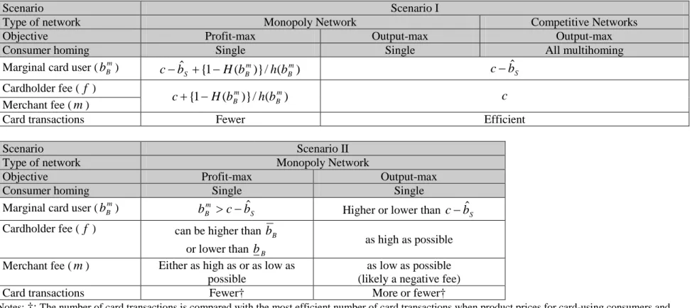
Table 3: Equilibrium Fee Structure: Discriminatory Pricing

Scenario Scenario I

Type of network Monopoly Network Competitive Networks

Objective Profit-max Output-max Output-max

Consumer homing Single Single All multihoming

Marginal card user (b_Bm) ˆ _{{1 ( )}/ (} m₎ B m B S H b h b b c− + − c−bˆS Cardholder fee ( f ) ) ( / )} ( 1 { m B m B h b b H c+ − c Merchant fee (m)

Card transactions Fewer Efficient

Scenario Scenario II

Type of network Monopoly Network

Objective Profit-max Output-max

Consumer homing Single Single

Marginal card user (b_Bm) m _S B c b

b > − ˆ Higher or lower than c−bˆ_S Cardholder fee ( f ) _{can be higher than}

B

b or lower than bB

as high as possible Merchant fee (m) Either as high as or as low as

possible

as low as possible (likely a negative fee)

Card transactions Fewer† More or fewer†

Notes: †: The number of card transactions is compared with the most efficient number of card transactions when product prices for card-using consumers and non-card-using consumers are the same. Thus, the number of card transactions is not necessarily the most efficient when merchants are allowed to set different prices for these two groups of consumers.

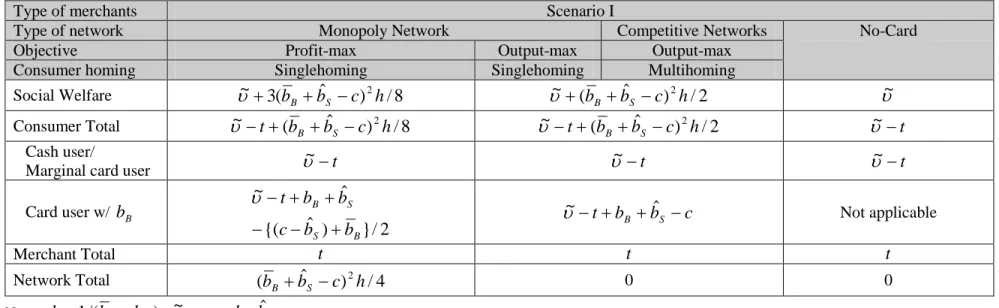
Table 4: Consumer, Merchant, and Network Surplus: Discriminatory Pricing

Type of merchants Scenario I

Type of network Monopoly Network Competitive Networks No-Card

Objective Profit-max Output-max Output-max

Consumer homing Singlehoming Singlehoming Multihoming

Social Welfare υ~+3(bB +bˆS −c)2h/8 ~ ( ˆ ) /2 2 h c b bB + S − + υ υ~ Consumer Total υ~−t+(b_B +bˆ_S −c)2h/8 υ~−t+(b_B +bˆ_S −c)2h/2 υ~−t Cash user/

Marginal card user υ −t

~ _υ~_{−t υ}~_−t Card user w/ bB 2 / } ) ˆ {( ˆ ~ B S S B b b c b b t + − − + + − υ c b b t+ _B + _S − − ˆ ~ υ Not applicable Merchant Total t t t Network Total (b_B +bˆ_S −c)2h/4 0 0 Notes: h=1/(bB −bB). d bˆS ~_{=υ− −} υ .

Table 4: Consumer, Merchant, and Network Surplus: Discriminatory Pricing (Cont.)

Type of merchants Scenario II

Type of network Monopoly Network No-Card

Objective Profit-max Output-max

Consumer homing Singlehoming Singlehoming

Social Welfare Higher than “No-Card” Higher than “Monopoly, Profit-Max” υ−bˆSt−d/(1−bˆS)

Consumer Total Higher than “No-Card” Higher than “Monopoly, Profit-Max” υ−t−d/(1−bˆS)

Cash user/

Marginal card user Same as “No-card” Same as “No-card” υ−t−d/(1−bˆS)

Card user w/ b_B Higher than “No-Card” cash user Higher than “No-Card” cash user and “Monopoly,

Profit-Max” Not applicable

Merchant Total Higher than “No-Card” Higher than “Monopoly, Profit-Max” (1−bˆ_S)t

Appendix A: Equilibrium Fee Structure

1: No-Discriminatory Pricing

Scenario I: Fixed Demand and Flat Costs and Fees

When both Merchants A and B accept the cards, they earn the same profit of t/2.

Furthermore, as long as each merchant takes the same strategy as its rival’s, each earns the same

profit of t/2.

Consider the highest merchant fee the monopoly card network can charge to the merchants.

Suppose Merchant A accepts the cards but Merchant B does not. Each merchant’s profit is:

)] ˆ )( ˆ ))( ( 1 )( ( )} ˆ ˆ ( 3 ) ( 1 [{ 2 1 2 S B m B m B S B m B A b f b m H b H b b f m b b H t t − + − − − − − − + = π , 2 )} ˆ ˆ ( 3 ) ( 1 { 2 1 m b f b f H t t B S B − + − − − = π ,

where bˆ_B is the average transactional benefit from cards among card-using consumers. When

merchant fee is m>bˆ_S +bˆ_B − f , Merchant B rejects the cards, given Merchant A accepts the cards. Given Merchant B rejects the cards, Merchant A rejects cards, too. When merchant fee is

f b b

m≤ ˆ_S + ˆ_B − , Merchant B does not reject cards, given Merchant A accepts the cards. Thus, the highest merchant fee the monopoly card network can charge is:

f b b m= ˆS + ˆB − . )) ( 1 )( (f +m−c −H f = Π

Profit-maximizing monopoly network

The profit-maximizing monopoly network solves the following problem:

Max , s.t. m≤bˆ_S +bˆ_B − f .

2 ) ˆ ( ˆ ˆ ˆ B S S B S b c b b f b b m= + − = + − − , and S b c f = − ˆ . ) ( 1−H f

Output-maximizing monopoly network

The output-maximizing monopoly network solves the following problem:

Max , s.t. f +m−c≥0 and m≤bˆS +bˆB − f .

When c−bˆS is large enough (i.e., c−bˆS ≥(bB +bB)/2), both constraints bind. The equilibrium

fee structure is:

) ˆ ( ˆ _{b b c} b m= S + B + S − , and ) ˆ ( ) ˆ (c b b b c f = − _S − _B + _S − .

However, if c−bˆ_S is small (i.e., c−bˆS <(bB +bB)/2), then the cardholder fee reaches the

consumers’ lowest transactional benefit from cards before the budget constraint binds. The

equilibrium fee structure in this case is:

2 ˆ B B S b b b m= + − , and B b f = .

Suppose two competing card networks, Network 1 and Network 2, are symmetric in terms

of their costs of processing card transactions and cardholder bases. The number of card

transactions increases as the cardholder fee decreases. Both networks reduce their markups to

lower their card holder fees, which means their total fee revenues per transaction is reduced to

their costs per transaction:

Output-maximizing competitive networks with all multihoming cardholders

c m f m

fee than Network 2 ( f1 > f2). If both merchants accept Network 2’s card (Card 2), then

consumers whose transactional benefit from cards exceeds f₂ use Card 2 only. Merchants A and

B earn the same profit of t/2. If Merchant A accepts both Cards 1 and 2 and Merchant B

accepts Card 1 only, then their profits are:

)}], )( 1 ( ) ~ )( ){( ˆ ( )} ( 3 1 ) ˆ ~ ( 3 [{ 2 1 2 1 1 2 2 1 2 2 2 2 2 1 1 1 2 2 2 1 f f H f b H H b m H m f m f H m f b b H H t t B S S B A − − + − − − − − − + − + − − + − + = π )}], ( ) ~ )( ){( ˆ )( 1 ( )} ( 3 1 ) ˆ ~ ( 3 [{ 2 1 2 1 2 1 2 1 1 1 2 2 2 1 1 1 2 2 2 1 f f H b f H H b m H m f m f H m f b b H H t t B S S B B − + − − − − + − − + − − − − + − − = π where H₁ = H(f₁), H₂ =H(f₂), and ~ 1 ( ) /( ( ₁) ( ₂)) 2 f H f H db b h b b f _{B B} f B B =

∫

f > _B > . If Network 2 sets m₂ =bˆ_S and f₂ =c−bˆ_S, rejecting Card 2 makes a merchant

worse off, given the other merchant accepts Card 2. It is also true that if Network 1 sets m₁ =bˆ_S

and f₁ =c−bˆ_S, accepting Card 2 makes a merchant worse off, given the other merchant rejects Card 2. The equilibrium fee structure is:

S b m m₁ = ₂ = ˆ , S b c f f1 = 2 = − ˆ .

Scenario II: Fixed Demand and Proportional Costs and Fees

In contrast to the case where per transaction costs and fees are fixed, the Hotelling

merchant’s profits are affected by the card fee structure and transactional benefit from cards,

even when each merchant takes the same strategy as its rival’s. When both merchants reject

S b d t p − + = 1 ,

And each earns profit π0:

2 0 ) ˆ 1 ( 2tπ = −bS t .

When both merchants accept cards, each sets its price at:

) 1 )( 1 )( ˆ 1 ( ) ˆ 1 ( )} 1 )( ˆ 1 ( { )} 1 )( 1 ( ) ˆ 1 {( H m b f H b d H b f H t H m H b p B S B S − − − + + − − − + + + − − + − = ,

and each earns profit πC:

) 1 )( ˆ )( 1 ( ) 1 )( ˆ ( ) ˆ 1 ( ) 1 )( ˆ )( ˆ ( )} 1 )( ˆ ( ) ˆ 1 {( 2 2 2 H f b m H b m b Htd H f b b m t H b m b t B S S B S S S C − − − − − − − − − − − − − − − − = π , where H =H(f).

Consider the highest merchant fee the monopoly card network can charge to the

merchants. Suppose Merchant A accepts the cards but Merchant B does not. Each merchant sets

its price at:

)] ˆ 1 /( )} 1 )( ˆ )( ˆ 1 ( 2 ) 1 )( ˆ ( ) ˆ 1 ( 3 { )} 1 )( ˆ ( 3 ) ˆ 1 ( 3 [{ 1 S B S S S S S A b d H f b b H b m b t H b m b A p − − − − − − − − − + − − − − = )] ˆ 1 /( } ) 1 ( ) ˆ )( ˆ 1 ( ) 1 )( ˆ )( ˆ 2 2 4 ( ) 1 )( ˆ ( 2 ) ˆ 1 ( 3 { } ) 1 )( ˆ )( ˆ ( ) 1 )( ˆ )( ˆ 2 3 ( ) 1 )( ˆ ( 3 ) ˆ 1 ( 3 [{ 1 2 2 2 S B S B S S S B S B S S S B b d H f b b H f b b m H b m b t H f b b m H f b b m H b m b A p − × − − − + − − − − − − − − − + − − − + − − − − − − − − − = where A=3{(1−bˆ_S)−(m−bˆ_S)(1−H)}−{(3−4m+bˆ_S)+(m−bˆ_S)(1−H)}(bˆ_B − f)(1−H). And each merchant earns the following profit, respectively,:

) 1 }( ) ˆ ( }{ ) 1 {( ) }( ) ˆ 1 {( 2tπ_A = −b_S p_A −d p_B − p_A +t H + −m p_A −d p_B −p_A +t+ b_B − f p_A −H

) 1 }( ) ˆ ( }{ ) ˆ 1 {( ) }( ) ˆ 1 {( 2tπ_B = −b_S p_B −d p_A− p_B +t H + −b_S p_B −d p_A− p_B +t− b_B − f p_B −H

It is difficult (if not impossible) to analytically obtain the highest merchant fee that

monopoly card networks can charge. However, numerical examples suggest that the highest

merchant fee is slightly less than the sum of the merchant’s transactional benefit and the average

consumer’s net transactional benefit, i.e., m ≅bˆ_S +bˆ_B − f .

)) ( 1 )( (f m c H f p + − − = Π

Profit-maximizing monopoly network

The profit-maximizing monopoly network solves the following problem:

Max , s.t. m≤m and ) 1 )( 1 )( ˆ 1 ( ) ˆ 1 ( )} 1 )( ˆ 1 ( { )} 1 )( 1 ( ) ˆ 1 {( H m b f H b d H b f H t H m H b p B S B S − − − + + − − − + + + − − + − = .

It is difficult to analytically solve the equilibrium fee structure; however, the numerical examples

suggest that the equilibrium fee structure is:

2 ) ˆ ( ˆ ˆ ˆ B S S B S b c b b f b b m m= ≅ + − = + − − , and S b c f ≅ − ˆ . ) ( 1−H f

Output-maximizing monopoly network

The output-maximizing monopoly network solves the following problem:

Max , s.t. f +m−c≥0 and m=m.

If c−bˆS is large enough (i.e., c−bˆS ≥(bB +bB)/2 ), then two constraints bind. The equilibrium

fee structure is:

) ˆ ( ˆ _{b b c} b m m= ≅ _S + _B + _S − , and

) ˆ ( ˆ _{b b c} b c f = − _S − _B + _S − .

If c−bˆ_S is small (i.e., c−bˆ_S <(b_B +b_B)/2 ), then the cardholder fee reaches the consumers’ lowest transactional benefit from cards before the budget constraint binds. The equilibrium fee

structure in this case is:

2 ˆ B B S b b b m= + − , and B b f = . c m f m f₁ + ₁ = ₂ + ₂ =

Output-maximizing competitive networks with all multihoming cardholders

As discussed in Scenario I , two competing symmetric card networks reduce their markup

to zero, i.e., . Suppose Network 1 sets the higher cardholder fee than

Network 2 ( f₁ > f₂), and Merchant A accepts both Cards 1 and 2 and Merchant B accepts Card 1 only. The equilibrium product prices in this case are:

} ) 2 ( ) 2 {( 4 1 1 4 4 2 1 3 3 2 2 2 1 1 d L K L K t L K L K L K L K p_A + + + − = , } ) 2 ( ) 2 {( 4 1 2 4 4 1 2 3 3 1 2 2 1 1 d L K L K t L K L K L K L K pB = ₋ + + + , where B B b f B S H m b hb db b H f m K (1 )(1 )(1 ) (1 ˆ ) (1 ) B ( ) 2 2 2 2 2 2 1 = − + − + − − −

∫

∫

∫

B B b f B S H m b hb db b H f m L (1 )(1 )(1 ) (1 ˆ ) (1 ) B ( ) 1 1 1 1 1 1 1= − + − + − − −

∫

∫

∫

∫

Since analytical solutions are difficult to obtain, we use numerical examples to examine the

equilibrium. Suppose Network 2 sets its cardholder fee at f₂ =c−bˆ_S and Network 1 sets its

cardholder fee slightly higher, i.e., f1 =c−bˆS +ε, whereε >0. Merchant B’s profit is likely

higher than the profit it would have accepted Card 2 and the profit it would have rejected both

cards. Thus, given the rival merchant accepts Card 2, accepting Card 1 only is the most

profitable than any other strategies, such as accepting Card 2 and rejecting both Cards 1 and 2.

In contrast to Scenario I, Merchant A’s profit is also likely higher than that when both merchants

accept Card 2. Thus, given the rival merchant accepts Card 1 only, accepting Card 2 is the most

profitable strategy.

In fact, Network 2’s number of card transactions is greater than Network 1’s. Knowing one

of the two merchants accept Card 2, Network 2 has no incentive to reduce its merchant fee;

rather, it would lower its cardholder fee further by raising its merchant fee. Although Network 1

would be able to make at least one merchant accept Card 1 only by reducing its merchant fee, it

would have a smaller number of transactions than that when it sets the same merchant fee (thus

cardholder fee) as Network 2’s. As a result, both networks have an incentive to reduce their

consumers is relatively high, both networks set their cardholder fees at the lowest transactional

benefit. Thus, the equilibrium fee structure is:

2 ˆ 2 1 B B S b b b m m = = + − , and B b f f1 = 2 = .

However, when the lowest transactional benefit for consumers is relatively low, the above

would not be equilibrium fee structure. When both networks set their merchant fees high enough,

Merchant B’s most profitable strategy changes from accepting Card 1 only to rejecting both

cards. At those merchant fees, given Merchant B rejects both cards, Merchant A’s most

profitable strategy is rejecting both cards. Thus, both networks may not set their merchant fees at

such a high level. The threshold level of the merchant fees depends on other variables, but it is

higher than the equilibrium merchant fee set by output-maximizing monopoly network.

) ˆ ( ˆ _{b b c} b m m= > S + B + S − , and ) ˆ ( ˆ _{b b c} b c f < − _S − _B + _S − .

Scenario III: Downward-Sloping Demand Curve and Flat Costs and Fees

In contrast to the previous two scenarios, where consumers make a fixed number of

purchases and thus transactions, it is difficult to obtain analytical solution when each consumer’s

demand function is downward-sloping. Even equilibrium product prices are difficult to obtain

when two merchants take different strategies. We are able to predict what the equilibrium fee

structure looks like by making an additional assumption when cards are provided by monopoly

networks; however, in order to predict the equilibrium fee structure when cards are provided by

examples used in this paper. Therefore, here we only examine the equilibrium fee structure when

cards are provided by monopoly networks.

We assume that if one of the two merchants rejects the cards, the card-rejecting merchant

changes its product price, but the card-accepting merchant keeps its price at the same price level

where both merchants accept the cards. The card-rejecting merchant’s profit derived under this

assumption is likely higher than the profit when both merchants change their product price.

Thus, the highest merchant fee the monopoly networks charge (m) is likely lower than the

highest merchant fee they charge (m) when both merchants adjust their product prices. As long

as monopoly card networks set the merchant fee at m, both merchants accept the cards. The

product price they set is:

tb H f b b p D tb f b b p D H b m H f b b p D t b d p B C B C S B C S C + − − + + − + − − + − − + + + = ) 1 )( ˆ ( ) ( } ) ˆ ( ) ( ){ 1 )( ˆ ( )} 1 )( ˆ ( ) ( { ˆ _, where D(pC)=a−bpC. B B b f B C db b h bb bf bp a c m f ) B{ } ( ) ( Max Π= + −

∫

Profit-maximizing monopoly network

m m≤ s.t. and tb H f b b p D tb f b b p D H b m H f b b p D t b d p B C B C S B C S C + − − + + − + − − + − − + + + = ) 1 )( ˆ ( ) ( } ) ˆ ( ) ( ){ 1 )( ˆ ( )} 1 )( ˆ ( ) ( { ˆ _.

Numerical examples suggest that the equilibrium fee structure is:

2 ) ˆ ( ˆ ˆ ˆ B S S B S b c b b f b b m m= ≈ + − = + − − , and S b c f ≅ − ˆ .