POLITECNICO DI TORINO
Repository ISTITUZIONALE
The Generalized Bin Packing Problem with bin-dependent item profits / Baldi, Mauro Maria; Giovanni, Luigi De; Perboli, Guido; Tadei, Roberto. - (In corso di stampa).
Original
The Generalized Bin Packing Problem with bin-dependent item profits
Publisher: Published DOI: Terms of use: openAccess Publisher copyright
(Article begins on next page)
This article is made available under terms and conditions as specified in the corresponding bibliographic description in the repository
Availability:
The Generalized Bin Packing Problem with bin-dependent item profits
Abstract
In this paper, we introduce the Generalized Bin Packing Problem with bin-dependent item profits (GBPPI), a variant
of the Generalized Bin Packing Problem. In GBPPI, various bin types are available with their own capacities and
costs. A set of compulsory and non-compulsory items are also given, with volume and bin-dependent profits. The
aim of GBPPI is to determine an assignment of items to bins such that the overall net cost is minimized.
The importance of GBPPI is confirmed by a number of applications. The introduction of bin-dependent item
profits enables the application of GBPPI to cross-country and multi-modal transportation problems at strategic and
tactical levels as well as in last-mile logistic environments.
Having provided a Mixed Integer Programming formulation of the problem, we introduce efficient heuristics that can effectively address GBPPI for instances involving up to 1000 items and problems with a mixed objective function. Extensive computational tests demonstrate the accuracy of the proposed heuristics. Finally, we present a case study of
a well-known international courier operating in northern Italy. The problem approached by the international courier
is GBPPI. In this case study, our methodology outperforms the policies of the company.
Keywords: Bin Packing problems, Generalized Bin Packing Problem, metaheuristic, last-mile logistics.
1. Introduction
The transportation services market is estimated to be worth approximately 3 trillion euros worldwide with a gross
value added (GVA) of 600 billion in the EU-28 at basic prices, corresponding to a weight of approximately 5% of the
total GVA [26]. In addition to their classical uses at the operational level, packing problems have recently appeared as
tools for modeling strategic and tactical decisions taken in the transportation and supply chain sectors [18, 52]. This has led to new problems, such as the variable size and cost bin packing [17], the multi-handler knapsack problem
under uncertainty [53], and the generalized bin packing problem [6].
In this paper, we introduce Generalized Bin Packing Problem with bin-dependent item profits (GBPPI), which is
a variant of Generalized Bin Packing Problem (GBPP). The aim of GBPP is to minimize the difference between the total cost of the bins used and the total profit from the loading of the items. In GBPPI profits accrued from the items
are bin-dependent, i.e., they vary according to the bin in which an item is loaded.
The contribution of this paper is threefold. First, we consider a typical setting of strategic and tactical managerial
decisions for large dispatching and logistics companies related to the subcontracting of their deliveries to third-party
introduce flexibility in their business models [1, 19]. On the other hand, the increase in freight volumes (and the consequent increase in subcontracting) in conjunction with an extreme customization of the delivery services (and the
related costs) force managers to carefully consider the cost and quality of service at the contract level. Flexibility, cost
reduction and high standard of service quality are conflictual objectives. Existing models for Last Mile delivery only
partially consider these objectives while addressing the combination of several subcontractors [52, 53]. We model
this managerial problem through GBPPI. The introduction of bin-dependent item profits allows the use of GBPPI in
cross-country and multi-modal transportation, where contracts between a firm and 3PL vectors are stipulated through
a trade-off [18, 58]. This trade-offcan be effectively modeled through the introduction of bin-dependent item profits. In these settings, heuristic approaches are consistently exploited to solve complex transportation problems [27, 12].
In these problems, 3PLs play a fundamental role, as reported in a recent survey [1] and in [40], where a case study
was presented with the aim of fostering challenging strategies among 3PLs.
The second contribution of our paper is to apply GBPPI to model a specific case study arising in the context of
Smart City and involving a well-known international courier operating in northern Italy. Every day, the courier collects
its customers demands to pick-up and deliver freight. Customers pay the courier, who is responsible for the entire
transportation process. The courier refers to a set of transportation companies (TCs) and selects those that have the
capacity to perform the pick-ups and deliveries using their own trucks. Therefore, on a daily scale, the courier must
decide which TCs to select for day service, the number of trucks to be used by the selected TCs, and the assignment
of pick-ups and deliveries to trucks. The final decision concerning this daily choice of courier must be reached within
a limited time (approximately 10 minutes) to ensure the prompt assignment of freight to vehicles chosen from the
selected TCs and, therefore, an efficient service.
Third, with regard to packing problems literature, the introduction of the bin-dependent profits provides a more flexible packing formulation that will enable to tackle the majority of real-world performance indicators and to address
problems with mixed objective functions. This new formulation consists of a more general objective function
consist-ing of two terms with different signs: 1) the total cost of the bins used to be minimized; and 2) the total bin-dependent profit of the selected items to be maximized. We provide an integer-programming model for GBPPI. Unfortunately,
the mere use of commercial solvers is not sufficient to find good solutions of this model in reasonable computational time for real-world scenarios. Thus, some efficient heuristics are introduced. In particular, we derive two constructive heuristics and two metaheuristics.
The remainder of this paper is organized as follows: in Section 2, we introduce the problem and review important
literature on packing problems on which GBPPI is based. In Section 3, the GBPPI model is described, and in Section 4 heuristics for addressing GBPPI are introduced. Instance sets and computational results are given in Section 5. In
2. Problem setting and literature review
Each instance of GBPPI consists of a set of items and a set of bins. Items can be compulsory (i.e., mandatory to
load) or non-compulsory, and are characterized by volume and profit, which depend on the available bins. Bins are
characterized by the capacity and cost of use, and are classified by type. All bins belonging to the same bin type have
the same capacity and cost. The aim of GBPPI is to load compulsory items and profitable non-compulsory items into appropriate bins in order to minimize net cost. This is the difference between the total cost of the bins used and the total profit accruing from the loading of the items. Unlike GBPP, profits from items are bin-dependent, i.e., they vary
according to the type of the bin into which an item is loaded.
The proposed problem reveals an interesting parallel with another problem addressed during ESICUP 2015 [25],
sponsored by the automobile manufacturer Renault. Although the two problems are similar in the common goal to
find an optimal assignment of items to bins, they are different in terms of problem structure and planning horizon. More details about the comparison of the two problems are given in Appendix A.
The oldest problem is Bin Packing Problem (BPP), which consists of a set of items to be loaded into bins of equal
size such that the number of bins used is minimum. This problem was first introduced in the 1970s [59, 32, 38, 37]. An
online variant of BPP was studied by Seiden [56], whereas Rhee and Talagrand [54] and Peng and Zhang [48] studied the problem in a stochastic setting. Bounds for BPP can be found in a number of works [42, 60, 29, 16, 15]. BPP has
also been addressed by means of column generation [61] and polynomial-time approximation schemes [20, 39].
Bin Packing with Rejection (BPR) is a variant of BPP where items can also be rejected. If an item is rejected, a
penalty is paid. Therefore, the goal is to minimize the number of bins used and the penalties for the rejected items. A
number of studies on BPR can be found in the literature [21, 10, 22].
Variable Sized Bin Packing Problem (VSBPP) is a generalization of BPP, which was proposed in the 1980s by
Friesen and Langston [31], and involves the introduction of bin types. Murgolo [45] and Epstein and Levin [23]
provided efficient approximation schemes for it. Lower bounds have been proposed by Monaci [44], Crainic et al. [17], Haouari and Serairi [34], Mohamed et al. [43], and Balogh et al. [9]. Monaci [44] and Haouari and Serairi [34]
studied exact algorithms, whereas heuristic approaches were adopted in [33, 35, 41]. The online variant has been discussed in a number of works [55, 57, 62, 24, 11], whereas the stochastic variant has recently been studied by Fazi
et al. [28] and Crainic et al. [18].
Generalized Bin Packing Problem (GBPP) is a generalization of previous bin packing problems, involving the
introduction of item profits as well as compulsory and non-compulsory items. Heuristics, and exact and approximate
algorithms can be found in [6, 8]. Online and stochastic variants have been discussed in [7, 50]. Finally, approximation
issues have been studied in [5].
3. The GBPPI model
• I: set of items
• n=|I|: number of items • IC⊆ I: set of compulsory items
• INC ⊆ I: set of non-compulsory items. Clearly,ICandINCare a partition of setI, i.e.,IC∪ INC=Iand
IC∩ INC=∅
• J: set of bins
• m=|J |: number of bins • T: set of bin types
• σ : J −→ T: indicator function, where given bin j∈ J, reveals its typet ∈ T, i.e.,σ(j) =tiif bin j ∈ J
belongs to typet∈ T
• pit: profit generated by itemi∈ Iwhen accommodated into a bin of typet∈ T
• wi: volume of itemi∈ I
• Ct: cost of a bin of typet∈ T
• Wt: capacity of a bin of typet∈ T
• Lt: minimum number of bins to be used of typet∈ T
• Ut: maximum number of bins to be used of typet∈ T
• U≤P
t∈TUt: maximum number of bins to be used
• S ⊆ J: set of bins used in a solution of GBPPI
• Wres(b) : b∈ S: residual volume of a bin for a solution of GBPPI. This is given by the capacity of binbminus
the sum of the volumes of the items loaded inb.
An optimal solution of an instance of GBPPI must satisfy the following requirements:
• The overall cost given by the difference between the cost of the bins used and the profits incurred by the loaded items is minimized.
• All compulsory items must be accommodated into some bins.
• The sum of the volumes of the items loaded into a bin cannot exceed the capacity of that bin.
• At leastLtand at mostUtbins of typet∈ T can be used.
• At mostUbins can be used in total.
In order to provide a model for GBPPI, we need to introduce the following binary variables:
xi j=
1 if itemi∈ Iis accommodated into bin j∈ J 0 otherwise (1) yj= 1 if bin j∈ Jis used 0 otherwise (2)
A model for GBPPI can then be formulated as follows: min X j∈J Cσ(j)yj− X j∈J X i∈I piσ(j)xi j (3) s. t. X i∈I wixi j≤Wσ(j)yj j∈ J (4) X j∈J xi j =1 i∈ IC (5) X j∈J xi j ≤1 i∈ INC (6) X j∈J:σ(j)=t yj≤Ut t∈ T (7) X j∈J:σ(j)=t yj≥Lt t∈ T (8) X j∈J yj≤U (9) yj∈ {0,1} j∈ J (10) xi j∈ {0,1} i∈ I, j∈ J (11)
The objective function (3) ensures that the solution minimizes the overall cost, given as the cost due to bin use
minus the profit from the loading of the items into the bins. Constraints (4) are the so-called capacity constraints
that ensure that the sum of the volumes of the items loaded into a bin does not exceed bin capacity. Constraints (5) ensure that all compulsory items are loaded, whereas constraints (6) state that non-compulsory items may or may not
be accommodated. Constraints (7)–(8) are bin usage constraints. Finally, constraints (10)–(11) force the variables
involved to be binary.
Model (3)–(11) inherits all the variables and constraints from the model for GBPP described in [6] except for the
objective function. Although the change in the objective function due to the introduction of bin-dependent item profits
might seem trivial at first glance, in Appendix B we show that this change strongly worsens the problem. In Appendix
B, we present a detailed comparison in further detail between GBPP and GBPPI using a commercial solver on the
corresponding models. The results showed that the solver provides smaller gaps when applied to GBPP in the same
computational time. Moreover, as we show in Section 4, the introduction of bin-dependent item profits implies a
relevant generalization of the constructive heuristics used to tackle both problems.
Finally, we wish to point out that the presence of bin usage constraints (7)–(9) and a limited numbermof bins might lead to infeasible solutions. As shown in [6], in order to ensure that the problem is feasible, a dummy bin with
4. Heuristics
In this section, we present efficient heuristics for addressing GBPPI. As mentioned in the introduction and will be shown in Appendix B, the use of commercial solvers is not sufficient to efficiently address the problem, in particular if fast solutions with a computational time of at most 10 minutes are required (i.e., the average time for reaching
decisions at the operational level). For this reason, we developed a series of heuristics useful for addressing GBPPI. The common principle of our heuristics is to address problems where the sign of the objective function can be either
positive, null, or negative. In previous bin-packing problems the goal was to minimize a single objective: the number
of bins used, the wasted space, etc. This implied an objective function which is always non-negative. Vice versa, in
generalized bin packing problems like the GBPP or the GBPPI, we deal with an objective function which terms can
have different signs. In fact, minimizing the net cost implies the optimization of two contributes: the minimization of the costs (which signs are non negative) and the maximization of the profits (which signs are non positive). As it will
be shown in this section, our heuristics take this broadening of the objective function into account. Thus, they are also
suitable to address those problems with a mixed target in the objective function. The proposed heuristics are:
• one constructive heuristic named Best profitable(BP)
• one constructive heuristic named BestAssignment(BA),
• one metaheuristic named Greedy Randomized Adaptive Search Procedure (GRASP) [30],
• a parallel metaheuristic named Model-Based Metaheuristic (MBM).
These heuristics provide a flexible trade-offbetween quality of solution and computational time, in light of the imposed maximum computational time of 10 minutes.
4.1. The constructive heuristics
The proposed constructive heuristics are a variant of BestFitDecreasing(BFD) introduced by Johnson et al.
[38] to address BPP. As already discussed, this generalization is necessary to address GBPPI and problems with a
mixed objective function. Our constructive heuristics are called Best profitable(BP) and BestAssignment(BA),
and operate with a list of available binsSBLand one of sorted itemsSIL. The major variant implemented in order to address GBPPI is the broadening of the definition of thebestbin. LetS ⊆ J be the set of bins used in a solution of a bin packing problem, and letWres(b) be the residual volume of binb∈ S. In previous versions of the bin-packing
problem, the best bin for an item was defined as the one that can accommodate the item such that the residual space
is minimized. In GBPPI, instead of considering the minimum residual space, we compute a figure of merit consisting
of a weighted sum that takes into account both item profit and bin volume. Again, this choice is motivated by the fact that in GBPPI, we need to consider two factors. In classical bin packing problems the aim is to minimize residual
space in order to reduce the number of bins used or the cost of bin usage. The adoption of this approach in GBPPI
does not always guarantee effective outcomes because item profits in such cases rely heavily on bins. Our weighted figure of merit, defined asα·piσ(j)−(1−α)·Wres(j), simultaneously addresses these two loading policies. The term
piσ(j) maximizes item profit, whereas the termWres(j) minimizes residual space. α ∈ [0,1] is a coefficient that is
varied during the execution of GRASP (cf. Section 4.2), and allows both loading policies to be spanned.
A further generalization is that this definition of the best bin is applied to a subset ofN |S IL|items, rather than a single item. When we consider itemiin listSIL, we take into account the sublistS IL0={i,i+1, . . . ,i+N−1}. For each item, we compute the best bin; at the end of this process, we select the best itemi∗∈S IL0and the best binb that maximizes the aforementioned figure of merit. Our computational experience confirmed that this “medium-term”
memory improves the performance of the heuristics. The behavioral difference between BP and BA heuristics can be observed when we cannot load itemi∈ S ILinto any of the already bins used inS. In this case, we try to select a new bin where to accommodate itemi. The BP heuristic considers itemiwith the remaining succeeding items in
S IL, and selects the bin that minimizes the difference between bin cost and the sum of profits from items that can be loaded into that bin. Similarly, the BA heuristic selects the bin that maximizes profit for itemi. Both heuristics perform a post-optimization procedure that tries to move items to cheaper bins and to remove non-profitable bins. It
is clear that the solutions provided by the BP and BA heuristics depend on the two parametersαandN. As we show in Section 4.2, the values of these parameters are varied using the GRASP procedure, which employs BP and BA as
sub-heuristics.
4.2. TheGRASP
Greedy Randomized Adaptive Search Procedure (GRASP) algorithms consist of a multi-start procedure to find
a good initial solution and of a loop where, at each iteration, a new solution is generated by means of a simpler
heuristic. In our GRASP for GBPPI, we employ the Best profitableand BestAssignmentheuristics, which were
already described in Subsection 4.1.
At each iteration of the main loop, we try to generate a different and improved solution by varying the order of the items in the listSIL. This is performed by associating ascorewith each item. A score update procedure randomly assigns a different score value to each item.
Finally, a long-term reinitialization procedure is executed each time a solution does not improve in consecutive
iterations. Its purpose is to explore a different area of the feasible set by changing parametersαandNof the construc-tive heuristics. The proposed method incorporates some ideas from [49]. The pseudo-code of our GRASP is proposed
in Algorithm 1.
The algorithm presented in this section satisfies the terminology of the term GRASP, namely Greedy Randomized
Adaptive Search Procedure. It is a greedy algorithm because it is based on the BP and BA procedures that can be
classified as greedy algorithms. It is also a randomized algorithm because randomization is present in the assignment
of scores. Finally, it is also an adaptive-search algorithm because the long-term reinitialization procedure is helpful to
explore new regions of the solution space.
The GRASP metaheuristic can be easily parallelized. LetPbe the set of available threads in a parallel
Algorithm 1The GRASP
1: IS: initial solution provided by themulti-start initializationprocedure 2: BS :=IS
3: numConsecutive: number of consecutive non-improving solutions 4: numConsecutive:=0
5: whiletime limit has not been reacheddo
6: sort the items
7: perform either the BP or the BA constructive heuristic
8: store the resulting solution asCS
9: ifCS <BS then 10: BS :=CS 11: numConsecutive:=0 12: else 13: numConsecutive:=numConsecutive+1 14: end if
15: score updateprocedure
16: ifnumConsecutive=MAXCONS ECUT IV Ethen
17: long-term reinitializationprocedure
18: numConsecutive:=0 19: end if
random-number generator. LetBP(p) be the final best solution provided by the GRASP executed by threadp ∈ P, then the overall best solutionBS will be
BS =min
p∈P BS(p).
4.2.1. Multi-start initialization
The purpose of our multi-start initialization procedure is twofold: to feed the main loop of GRASP with a good
initial solution, and automatically calibrate the parameters used by the constructive heuristics. The three parameters
involved in GRASP areα,N, andNmax, whereNmaxis the maximum of parameterN. The first two parameters are used
in constructive heuristics, as previously discussed, whereas the latter is only updated in the long-term reinitialization
procedure.
In multi-start initialization, we executeM=min{25,n}Best profitableheuristics 100 times, withNvarying from 1 toM, andαinitially set to 0.25. The value ofNcorresponding to the best solution found during theMiterations is set as the maximum dimensionNmax.
4.2.2. Score update
Item scores are randomly extracted from a discrete uniform distribution in the range [0,4n]. The motivation for this choice is that working with integer values rather than real values implies a faster resolution of the sorting
procedure. We prefer to distribute the item scores in a range proportional to the number of items, and then use integer
scores rather than concentrating the scores with real values within a smaller range.
4.2.3. Long-term reinitialization
An index is incremented modulo 5, andαis set to the corresponding position in set{0.25,0.4,0.5,0.6,0.75}. Moreover, the parameterN of the group of items used in constructive heuristics is incremented. Nis set to 1 again after it reaches the maximum dimension allowedNmax.
4.3. The Model-Based Metaheuristic
We present here a parallel metaheuristic for GBPPI, where a set of computer threadsPrun simultaneously. It
consists of a loop, where at each iteration each thread solves a subproblem using model (3)–(11). The resolution of
subproblems with model (3)–(11) allows us to take into account two targets at the same time, namely the minimization
of the cost and the maximization of the profits. Thus, this metaheuristic is suitable to address problems with a similar structure.
In each subproblem, a small set of bins is randomly selected from the incumbent solution and the set of available
bins. In order to further improve the given solution, we merge couples of partial solutions that do not have any bins
and items in common. The best solution is updated if the new solution is an improvement over the incumbent one.
According to the taxonomy of parallel methods proposed by Crainic and Toulouse [14], this approach can be classified as 1C/RS/MPSS, where the following hold:
• 1C: One Control, i.e., one master thread controls all the remaining threads.
• RS: Rigid Synchronization, i.e., at each iteration, we wait for all threads to complete their computations.
• MPSS: Multiple points same strategy, i.e., each thread solves a different subproblem, but using the same strat-egy.
We chose to use this kind of parallelism because it can easily be implemented in our metaheuristic. As we show in the
next section, although the metaheuristic can be exploited without parallel computation, this approach is strongly
rec-ommended when GBPPI is employed as a subproblem of a larger problem, and significantly improves the performance
of the metaheuristic. The main steps of the MBM metaheuristic are shown in Algorithm 2.
Algorithm 2The MBM metaheuristic 1: P: set of threads
2: IS: Initial solution provided to the MBM metaheuristic 3: BS: Best solution
4: BS :=IS
5: whiletime limit has not been reacheddo
6: for allp∈ Pdo
7: Randomly select a subsetb(p) of bins from the set of binsSmaking up solutionBS.
8: Solve a GBPPI subproblem with a solver with a time limit of 1 s, the binsb(p) plus selected available bins, the items loaded into binsb(p), and the items not loaded in solutionBS.
9: end for
10: Merge partial solutions provided by each thread and store the new current solution inCS. 11: ifCS <BS then
12: BS :=CS
13: end if
14: end while
5. Computational results
As there are no instances for GBPPI in the literature, we have created new instance sets, starting from instances
of GBPP (cf. [6]). At the same time, instances of GBPP are based on Monaci’s VSBPP instances [44]. To make this
article self contained, we report here the details of both VSBPP and GBPP instances.
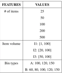
Monaci’s instances for the VSBPP consist of a group of 300 instances where the items are all compulsory. Table 1
FEATURES VALUES # of items 25 50 100 200 500
Item volume I1: [1, 100]
I2: [20, 100]
I3: [50, 100]
Bin types A: 100, 120, 150
B: 60, 80, 100, 120, 150
Table 1: Description of Monaci’s instances for VSBPP.
Ten instances were generated for each combination of features in Table 1, for a total of 5×3×2×10=300 instances. For each instance, the minimum and the maximum number of available bins for bin typet∈ T is respectively set to
Lt=0, ∀t∈ T Ut= lPi∈Iwi Wt m , ∀t∈ T.
GBPP instances consist of four classes of instances numbered from 0 to 3. Class 0 coincides with the instances
in Monaci [44] for VSBPP. Instances of classes 1 and 2 are identical to those belonging to class 0 but the profits. In
fact, in class 0 the items are all compulsory. Vice versa, in classes 1 and 2 the items are all non compulsory. The profit
piof itemi∈ Ibelonging to an instance in class 1 or 2 is given by
pi∈ dU(0.5,3)wie class 1,
pi∈ dU(0.5,4)wie class 2
respectively, whereUdenotes uniform distribution. Finally, Class 3 is a 500-item class, with 60 instances selected
from classes 0–2 with 0%, 25%, 50%, 75%, and 100% of compulsory items. GBPP instances are available on line [47].
Beginning with a selection of instances of GBPP, we created 600 instances for GBPPI while maintaining the same
values, but with item profits computed as
with θt=max l∈L ( 0.4CminCmax Wt ϑ ) , (12)
whereϑcan either be extracted from a uniform distributionU(0,1) or from a Gumbel distributionG(0,1). Values in (12) ensure that profit values approximate realistic settings. For the sake of brevity, we refer to instances of GBPPI
with item profits extracted from a Gumbel distribution according to (12) as Gumbel instances, and instances of GBPPI
with item profits extracted from a uniform distribution according to (12) as uniform instances. GBPPI instances are
also available on line [46].
Computational resources were provided byhpc@polito[36], on a system with Opteron 2.3 GHz processors and
124 GB of RAM. The metaheuristic was implemented in C++, with eight threads and with the following time limits: 1s for the GRASP, 1s for each subproblem solved with the solver, and 120s for the metaheuristic. We used the
commercial solver CPLEX 12.6 [13] to solve each subproblem and for the comparison between the GBPP and the
GBPPI (see Appendix B)
In Table 2, we list the percentage gaps between the algorithms proposed in this paper and the best solution found
by the solver in one hour. The results are reported according to the type of instance (Gumbel and uniform), the number
of items (from 25 to 200), and the number of threads (one and eight). We also wanted to estimate the benefits of a
parallel computation in comparison with a single-thread approach. The columns in Table 2 describe the following:
col. 1) is the type of distribution for item profits; col. 2) shows the number of items; col. 3) shows the percentage gap
in the best constructive heuristic with respect to the solver with one thread; cols. 4) – 5) are the percentage gaps of
GRASP and the MBM with one thread with respect to the solver with one thread; and cols. 6) – 7) are the percentage gaps of GRASP and the MBM with eight threads with respect to the solver with eight threads. The best constructive
heuristic was given by the minimum of the Best profitableand BestAssignmentheuristics.
The aim of column 3 is to show the performances of these constructive heuristics, which were executed with
α= 0.5 in order to emphasize both components in the figure of merit, and with the items sorted by non-increasing mean profits over volume. The best constructive heuristic was compared to the solver with one thread only because
the execution of Best profitableand the BestAssignmentheuristic does not require parallelism. The computational
time of the constructive heuristic was practically zero, but this immediate execution was paid for in terms of the
highest percentage gaps. In fact, the overall gap was 12.76%. Although this value was high, the Best profitable and BestAssignmentheuristics found their utility in the execution of GRASP and MBM, which yielded much lower
percentage gaps. Moreover, from Table 2 we can also observe the benefits of introducing parallelism. The percentage gap of GRASP was almost halved when switching from one to eight threads. This gap reduced from 4.08% to 2.82%,
which is a considerably improved result if we consider that the computational time of the GRASP was approximately
1 second. The percentage gaps of the MBM were satisfactory. Again, parallelism improved quality of solution. In
DISTRIBUTION ITEMS CONSTR.
1 THREAD 8 THREADS
GRASP MHEUR GRASP MHEUR
GUMBEL 25 13.07 0.97 0.10 0.86 0.02 50 15.05 3.94 0.16 2.69 0.14 100 14.76 5.69 0.39 4.66 0.31 200 13.77 6.89 0.12 4.56 -0.02 500 9.98 2.99 -1.95 1.03 -2.94 OVERALL 13.32 4.10 -0.24 2.76 -0.50 UNIFORM 25 14.28 1.03 0.05 0.97 0.04 50 14.06 3.71 0.24 2.89 0.17 100 12.56 5.93 0.41 4.52 0.39 200 11.86 7.24 0.19 5.01 0.16 500 8.24 2.44 -2.19 1.04 -2.97 OVERALL 12.20 4.07 -0.26 2.89 -0.44 OVERALL 12.76 4.08 -0.25 2.82 -0.47
Table 2: Percentage gaps in the proposed algorithms reported according to item profit distribution (column 1), number of items (column 2), and parallelism (columns 4–7).
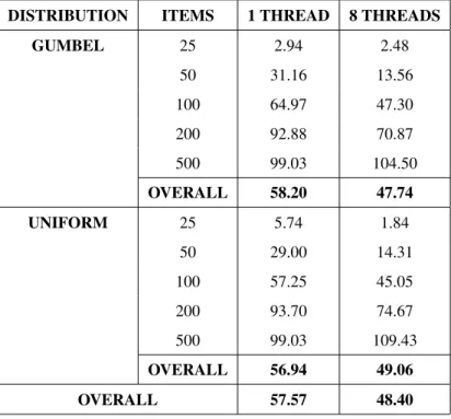
Table 3 presents the average computational times of the last best solution found by the MBM. The columns in Table 3 indicate the following: col. 1) represents the type of distribution for the item profits, col. 2) shows the number
of items, cols. 3) and 4) list the average computational times needed to find the best solution for the MBM with one
and eight threads, respectively.
DISTRIBUTION ITEMS 1 THREAD 8 THREADS
GUMBEL 25 2.94 2.48 50 31.16 13.56 100 64.97 47.30 200 92.88 70.87 500 99.03 104.50 OVERALL 58.20 47.74 UNIFORM 25 5.74 1.84 50 29.00 14.31 100 57.25 45.05 200 93.70 74.67 500 99.03 109.43 OVERALL 56.94 49.06 OVERALL 57.57 48.40
Table 3: Best computational times for the MBM reported according to item profit distribution (column 1), number of items (column 2), and parallelism (columns 3–4).
The analysis of Table 3 reveals that the average time tended to increase in line with instance size. Moreover, the
overall average time was approximately one minute.
Finally, we compared the MBM with the branch-and-price by Baldi et al. [8] on the same instances as the classical
GBPP. We computed the percentage gaps of the MBM with respect to the branch-and-price results. The results are
presented in Table 4 according to the number of items. In particular, columns 2, 4, 6, and 8 indicate the percentage
gaps of the branch-and-price with respect to its best lower bound computed at the root node (cf. [8] for further details).
Columns 3, 5, 7, and 9 present the percentage gaps of the MBM with respect to the best objective function provided
by the branch-and-price. The instances in Class 3 were defined for 500 items only. The overall percentage gap of the MBM compared to the branch-and-price was approximately 0.22%. Nevertheless, we observed that for 34 instances,
better results were found than those provided by the branch-and-price in Baldi et al. [8], and within a considerably
smaller computational time. The time limit of the branch-and-price was one hour, while that of the MBM was two
minutes. Moreover, for a third of the instances of GBPP, the Model-Based Metaheuristic could find the same results
ITEMS CLASS 0 CLASS 1 CLASS 2 CLASS 3
BEP MHEUR BEP MHEUR BEP MHEUR BEP MHEUR
25 0.00 0.01 0.00 0.02 0.00 0.00 *** *** 50 0.00 0.19 0.00 0.14 0.01 0.12 *** *** 100 0.02 0.32 0.03 0.26 0.01 0.15 *** *** 200 0.06 0.33 0.02 0.37 0.03 0.28 *** *** 500 0.12 0.38 0.12 0.34 0.11 0.26 0.57 0.59 OVERALL 0.04 0.25 0.03 0.23 0.03 0.16 0.57 0.59
Table 4: Comparisons between the branch and price and the MBM. Columns 2, 4, 6, and 8 show the percentage gap of the branch and price with respect to the best lower bound. Columns 3, 5, 7, and 9 show the percentage gap of the MBM with respect to the best objective function provided by the branch and price. *** The instances in Class 3 were defined for 500 items only.
6. Smart City case study
As described in the Introduction, the case study referred to the planning of pick-up and delivery operations of an
international courier. The decisions of the courier arose from a competitive tender between the courier and
transporta-tion companies (TCs). In this competitive tender, each TC proposes a transportatransporta-tion cost for each truck used. This
cost covered expenses such as drivers, fuel, and depreciation in vehicle value. Moreover, a TC received a bonus for
each successful pick-up or delivery. The courier selected TCs according to the proposed transportation costs and TC
reliability. The courier migh have checked the quality of each shipment through truck inspection and feedback from
customers. Drivers who did not load the freight into the truck correctly, or customers who filed a complaint with the courier regarding a delayed or missed delivery, or for receiving a damaged product, clearly reduced the reliability of
a TC. Conversely, prompt pick-ups and deliveries and positive feedback from customers increased the reliability of
a TC. The higher TC reliability, the higher customer satisfaction. Therefore, the profit for the courier in shipping a
freight was not only proportional to the economic value of the freight, but also to the TC reliability.
In our case study, the set of itemsIrepresented the freight that the courier needed to pick-up and deliver. The
different bin types represented the available TCs, the bins were the trucks, andUtis the cardinality of the fleet of the
TCt∈ T. Item revenues consisted of the sum of two terms,ρiandχσ(j), whereρiwas the economic value of shipping
itemi∈ I, andχσ(j)was the gain due to the reliability of TC j∈ J. A bonuscσ(j) was awarded to the TC for each
shipment with a truck of typeσ(j). Therefore, item profits becamepiσ(j) =ρi+χσ(j)−cσ(j).
In the case study, we compare our MBM solutions with those of the courier based on its business policy. We
analyzed 30 instances (i.e., 30 competitive tenders) with 1,000 daily pick-ups and deliveries (i.e., the items), 10 TCs
(i.e., the bin types), and up to 100 trucks (i.e., the bins) per TC, available in a distribution area located in northern
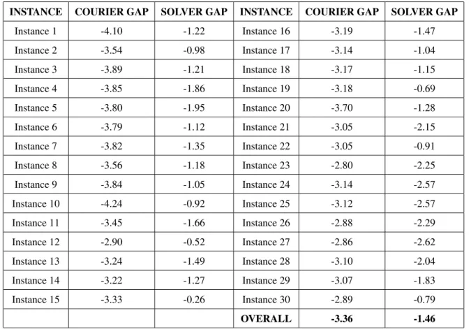
In Table 5, we present the percentage gaps of our MBM compared to the business policy and the solver (this time with a time limit of two hours) over the 30 competitive tenders. Our MBM always found better results than those
provided by the business policy and the solver.
INSTANCE COURIER GAP SOLVER GAP INSTANCE COURIER GAP SOLVER GAP
Instance 1 -4.10 -1.22 Instance 16 -3.19 -1.47 Instance 2 -3.54 -0.98 Instance 17 -3.14 -1.04 Instance 3 -3.89 -1.21 Instance 18 -3.17 -1.15 Instance 4 -3.85 -1.86 Instance 19 -3.18 -0.69 Instance 5 -3.80 -1.95 Instance 20 -3.70 -1.28 Instance 6 -3.79 -1.12 Instance 21 -3.05 -2.15 Instance 7 -3.82 -1.35 Instance 22 -3.05 -0.91 Instance 8 -3.56 -1.18 Instance 23 -2.80 -2.25 Instance 9 -3.84 -1.05 Instance 24 -3.14 -2.57 Instance 10 -4.24 -0.92 Instance 25 -3.12 -2.57 Instance 11 -3.45 -1.66 Instance 26 -2.88 -2.29 Instance 12 -2.90 -0.52 Instance 27 -2.86 -2.62 Instance 13 -3.24 -1.49 Instance 28 -3.10 -2.04 Instance 14 -3.22 -1.27 Instance 29 -3.07 -1.83 Instance 15 -3.33 -0.26 Instance 30 -2.89 -0.79 OVERALL -3.36 -1.46
Table 5: Percentage gaps of the MBM compared with the business policy and the solver. Columns 1 and 4 present the instance number of the case study, columns 2 and 5 the percentage gaps of the business policy compared to the MBM, and columns 3 and 6 the percentage gaps of the solver compared to the MBM.
A more interesting outcome results from the analysis of the instances from an economic and managerial point of
view. The size of each instance was representative of the daily parcels of a parcel delivery company in a
medium-sized city. If we compare the solution with one based on expert opinion (tactical decisions based on expert opinion and
day-to-day decisions optimized by means of specific optimization tools), the assignments given by GBPPI achieve a
constant reduction of the overall cost by between 3 and 4%. In terms of the economic impact of costs, this amounts to 120,000–180,000 euros for a city the size of Turin (the interval depends on different scenarios of annual numbers of parcels). Moreover, this cost will increase in the near future, due to increase in B2C flows resulting from e-commerce,
mass customization, and decentralized production. This leads to problems that are not solvable based simply on
expert opinion. The increase in volumes in the B2C market goes hand in hand with a reduction in the marginal
of deliveries [2, 3, 4].
7. Conclusions
In this paper, we introduced a new packing problem named Generalized Bin Packing Problem with bin-dependent
item profits (GBPPI). We have shown that GBPPI can be applied at both tactical and operational levels. At the tactical level, GBPPI models cross-country and multi-modal transportation settings. At an operational level, GBPPI describes
the problem of a courier selecting the appropriate number and type of vehicles from a set of available transportation
companies. We have also demonstrated that the introduction of bin-dependent item profits is not trivial in terms of
problem resolution. We presented a number of heuristics to efficiently address the problem within limited computa-tional time. We have also presented extensive computacomputa-tional results and a case study of a well-known internacomputa-tional
courier operating in northern Italy.
GBPPI can also be a starting point for future research. In fact, GBPPI can be exploited as a subproblem in
the resolution of the stochastic variant of GBPP, namely Stochastic Generalized Bin Packing Problem. Stochastic
problems are affected by uncertainty. The Progressive Hedging Algorithm is an iterative technique for addressing these problems [19]. At each iteration, random variables describing uncertain attributes are fixed to particular values. In this way, each iteration of the Progressive Hedging Algorithm applied to Stochastic Generalized Bin Packing
Problem implies the solution of a deterministic GBPPI subproblem. This solution may successfully be performed
through the heuristics proposed in this article.
Acknowledgments
Partial funding for this project was provided by the SYNCHRO-NET project, H2020-EU.3.4. - Societal
Chal-lenges - Smart, Green and Integrated Transport, ref. 636354 and by the UrbeLOG project, Smart Cities and
Commu-nities program, Italian University and Research Ministry.
References
[1] A. Aguezzoul. Third-party logistics selection problem: A literature review on criteria and methods.Omega, 49:69–78, 2014. [2] Amazon-com, Inc. Annual report 2013. U.S. securities and exchange commission report, 2014.
[3] Amazon-com, Inc. Annual report 2014. U.S. securities and exchange commission report, 2015. [4] Amazon-com, Inc. Annual report 2015. U.S. securities and exchange commission report, 2016.
[5] M. M. Baldi and M. Bruglieri. On the generalized bin packing problem.ITOR, 2016. doi: 10.1111/itor.12258. DOI 10.1111/itor.12258. [6] M. M. Baldi, T. G. Crainic, G. Perboli, and R. Tadei. The generalized bin packing problem.Transportation Research Part E, 48(6):1205–1220,
2012. doi: 10.1016/j.tre.2012.06.005.
[7] M. M. Baldi, T. G. Crainic, G. Perboli, and R. Tadei. Asymptotic results for the generalized bin packing problem. Procedia - Social and Behavioral Sciences, 111:663–671, 2013. doi: 10.1016/j.sbspro.2014.01.100. DOI 10.1016/j.sbspro.2014.01.100.
[8] M. M. Baldi, T. G. Crainic, G. Perboli, and R. Tadei. Branch-and-price and beam search algorithms for the variable cost and size bin packing problem with optional items. Annals of Operations Research, 222(1):125–141, 2014. doi: 10.1007/s10479-012-1283-2. DOI 10.1007/s10479-012-1283-2.
[9] J. Balogh, J. B´ek´esi, and G. Galambos. New lower bounds for certain classes of bin packing algorithms. Theoretical Computer Science, 440–441:1–13, 2012.
[10] W. Bein, J. R. Correa, and X. Han. A fast asymptotic approximation scheme for bin packing with rejection.Theoretical Computer Science, 393:14–22, 2008.
[11] J. Boyar and L. M. Favrholdt. A new variable-sized bin packing problem.Journal of Scheduling, 15:273–287, 2012.
[12] M. Caramia and F. Guerriero. A heuristic approach to long-haul freight transportation with multiple objective functions. Omega, 37(3): 600–614, 2009.
[13] CPLEX 12.6. URL http://www.ibm.com/support/knowledgecenter/SSSA5P_12.6.2/ilog.odms.cplex.help/CPLEX/ homepages/CPLEX.html.
[14] T. G. Crainic and M. Toulouse. Parallel Meta-heuristics. In M Gendreau and J-Y Potvin, editors,Handbook in Metaheuristics, pages 497–542. Kluwer Academic Publishers, Norwell, MA, 2010.
[15] T. G. Crainic, G. Perboli, M. Pezzuto, and R. Tadei. Computing the asymptotic worst-case of bin packing lower bounds.European Journal of Operational Research, 183:1295–1303, 2007.
[16] T. G. Crainic, G. Perboli, M. Pezzuto, and R. Tadei. New bin packing fast lower bounds.Computers&Operations Research, 34:3439–3457, 2007. doi: 10.1016/j.cor.2006.02.007.
[17] T. G. Crainic, G. Perboli, W. Rei, and R. Tadei. Efficient lower bounds and heuristics for the variable cost and size bin packing problem.
Computers&Operations Research, 38:1474–1482, 2011.
[18] T. G. Crainic, L. Gobbato, G. Perboli, W. Rei, J. P. Watson, and D. L. Woodruff. Bin packing problems with uncertainty on item characteristics: An application to capacity planning in logistics.Procedia - Social and Behavioral Sciences, 111:654–662, 2014.
[19] T. G. Crainic, L. Gobbato, G. Perboli, and W. Rei. Logistics capacity planning: A stochastic bin packing formulation and a progressive hedging meta-heuristic.EUROPEAN JOURNAL OF OPERATIONAL RESEARCH, 253:404–417, 2016. doi: http://dx.doi.org/10.1016/j.ejor. 2016.02.040.
[20] W.F. de la Vega and G.S. Lueker. Bin packing can be solved within 1+in linear time.Combinatorica, 1(4):349–355, 1981.
[21] G. D´osa and Y. He. Bin packing problems with rejection penalties and their dual problems.Information and Computation, 204(5):795–815, 2006.
[22] L. Epstein. Bin packing with rejection revisited.Algorithmica, 56(4):505–528, 2010.
[23] L. Epstein and A. Levin. Bin packing with general cost structures.Mathematical Programming, 132:355 – 391, 2012.
[24] L. Epstein, L. M. Favrholdt, and A. Levin. Online variable-sized bin packing with conflicts.Discrete Optimization, 8(2):333 – 343, 2011. [25] ESICUP. Challenge ESICUP 2015, 2015. URLhttp://challenge-esicup-2015.org/.
[26] European Commission: Energy and Transport. EU transport in figures: 2015. Technical report, Publications Office of the European Union, 2015.
[27] J. Faulin. Applying{MIXALG}procedure in a routing problem to optimize food product delivery.Omega, 31(5):387–395, 2003.
[28] S. Fazi, T. van Woensel, and J. C. Fransoo. A stochastic variable size bin packing problem with time constraints. Technical report, Technische Universiteit Eindhoven, 2012.
[29] S. P. Fekete and J. Schepers. New classes of lower bounds for bin packing problems.Mathematical Programming, 91(1):11–31, 2001. [30] P. Festa and M. G. C. Resende. Grasp: basic components and enhancements.Telecommunication Systems, 46(3):253–271, 2011. [31] D. K. Friesen and M. A. Langston. Variable sized bin packing.SIAM Journal on Computing, 15:222–230, 1986.
[32] M. R. Garey, R. L. Graham, and J. D. Ullman. Worst-case analysis of memory allocation algorithms. InProceedings of the fourth annual ACM symposium on Theory of computing, STOC ’72, pages 143–150, New York, NY, USA, 1972.
[34] M. Haouari and M. Serairi. Relaxations and exact solution of the variable sized bin packing problem. Computational Optimization and Applications, 48:345–368, 2011.
[35] V. Hemmelmayr, V. Schmid, and C. Blum. Variable neighbourhood search for the variable sized bin packing problem. Computers& Operations Research, 39:1097–1108, 2012.
[36] HPC@POLITO. A project of academic computing within the department of control and computer engineering at the politecnico di torino (http://www.hpc.polito.it).
[37] D. S. Johnson.Near-Optimal bin packing algorithms. PhD thesis, Dept. of Mathematics, M.I.T., Cambridge, MA, 1973.
[38] D. S. Johnson, A. Demeters, J. D. Hullman, M. R. Garey, and R. L. Graham. Worst-case performance bounds for simple one-dimensional packing algorithms.SIAM Journal on Computing, 3:299–325, 1974.
[39] N. Karmarkar and R. M. Karp. An efficient approximation scheme for the one-dimensional bin packing problem. InProceedings of 23rd Annual Symposium on Foundations of Computer Science, pages 312–320. IEEE Comput. Soc. Press., 1982.
[40] C. Kim, K. H. Yang, and J. Kim. A strategy for third-party logistics systems: A case analysis using the blue ocean strategy.Omega, 36(4): 522–534, 2008.
[41] M. Maiza, A. Labed, and M. S. Radjef. Efficient algorithms for the offline variable sized bin-packing problem.Journal of Global Optimization, 2013.
[42] S. Martello and P. Toth.Knapsack Problems - Algorithms and computer implementations. John Wiley & Sons, Chichester, UK, 1990. [43] M. Mohamed, R. M. Said, and S. Lakhdar. Continuous lower bound for the variable sized bin-packing problem. In9th International
Conference on Modeling, Optimization&SIMulation, June 2012, Bordeaux, France, 2012.
[44] M. Monaci.Algorithms for packing and scheduling problems. PhD thesis, Universit`a di Bologna, Bologna, Italy, 2002.
[45] F. D. Murgolo. An efficient approximation scheme for variable-sized bin packing.SIAM Journal on Computing, 16:149–161, 1987. [46] ORO group. Gbppi instances, . URLhttps://bitbucket.org/ORGroup/gbppi_instances.
[47] ORO group. Gbpp istances, . URLhttps://bitbucket.org/ORGroup/01_gbpp_instances.git.
[48] J. Peng and B. Zhang. Bin packing problem with uncertain volumes and capacities. http://orsc.edu.cn/online/120601.pdf, 2012.
[49] G. Perboli, T. G. Crainic, and R. Tadei. An efficient metaheuristic for multi-dimensional multi-container packing. InAutomation Science and Engineering (CASE), 2011 IEEE Conference on Automation Science and Engineering, pages 563 –568, 2011. doi: 10.1109/CASE.2011. 6042476.
[50] G. Perboli, R. Tadei, and M. M. Baldi. The stochastic generalized bin packing problem. Discrete Applied Mathematics, 160:1291–1297, 2012.
[51] G. Perboli, A. De Marco, F. Perfetti, and M. Marone. A new taxonomy of smart city projects.Transportation Research Procedia, 3:470–478, 2014.
[52] G. Perboli, L. Gobbato, and F. Perfetti. Packing problems in transportation and supply chain: new problems and trends.PROCEDIA - Social and Behavioral Sciences, 111:672–68, 2014.
[53] G. Perboli, R. Tadei, and L. Gobbato. The multi-handler knapsack problem under uncertainty. European Journal of Operational Research, 236(3):1000–1007, 2014.
[54] W. T. Rhee and M. Talagrand. On line bin packing with items of random size.Mathematics of Operations Research, 18(2):438–445, 1993. [55] S. Seiden. An optimal online algorithm for bounded space variable-sized bin packing. In Ugo Montanari, Jos Rolim, and Emo Welzl, editors,
Automata, Languages and Programming, volume 1853 ofLecture Notes in Computer Science, pages 283–295. Springer, 2000. [56] S. Seiden. On the online bin packing problem.Journal of the ACM, 49(5):640–671, 2002.
[57] S. S. Seiden, R. Van Stee, and L. Epstein. New bounds for variable-sized online bin packing.SIAM Journal on Computing, 32(2):455–469, 2003.
[58] R. Tadei, G. Perboli, and M. M. Baldi. The capacitated transshipment location problem with stochastic handling costs at the facilities.
International Transactions in Operational Research, 19(6):789–807, 2012.
[60] A. van Vliet. An improved lower bound for on-line bin packing algorithms.Info Process. Lett., 43(5):277–284, 1992.
[61] F. Vanderbeck. Computational study of a column generation algorithm for bin packing and cutting stock problems.Mathematical Program-ming, 86:565–594, 1996.
[62] G Zhang. A new version of on-line variable-sized bin packing.Discrete Applied Mathematics, 72(3):193 – 197, 1997.
Appendix A. Comparisons between GBPPI and the ESICUP 2015 problem
The ESICUP 2015 context dealt with a container-loading problem to be considered by Renault for the daily
loading of containers, and to “estimate every week the number of containers needed for the following weeks.” There
is an interesting number of analogies between GBPPI and the ESICUP 2015 problem. Both the problems deal with
assignment of items to bins. Moreover, the items are not necessarily compulsory. In fact, the least profitable items
can be put aside and be packed in the next shipment. Despite these analogies, we note that the two problems are quite
different. In particular, the ESICUP 2015 problem is a three-dimensional bin packing problem. For each bin, items can be packed into stacks. Stacks consist of layers, and layers consist of rows. Particular rotations of the items are
allowed, and both capacity and weight constraints need to be satisfied. Another big difference can be noticed in the objective functions of the two problems. GBPPI minimizes the overall net cost. The ESICUP 2015 problems presents
a lexicographic objective function, which main objective is the minimization of the wasted space. Finally, GBPPI is
a one-dimensional problem, which is characterized by the introduction of item profits that depend on the bins. This
dependency, which is not present in the ESICUP 2015 problem, also allows the use of GBPPI at a tactical level, as
discussed in Section 1.
Appendix B. Comparisons between GBPP and GBPPI
We compare here the classical version of GBPP with the new GBPPI. This comparison allows us to reveal two
important considerations. First, as GBPPI is a further generalization of the classical GBPP, higher computational
effort is required for it. Second, for this reason, it is important to design a heuristic that is accurate and fast at the same time, in order to be able to exploit the benefits of GBPPI in a city logistics setting, as discussed in the Introduction. In
city logistics decisions usually must be reached within a short time.
To make the comparison, we selected 30 instances of GBPP along with the corresponding Gumbel and uniform
instances of GBPPI, as explained in the text. Thus, the number of instances in this instance set is 90. The number
of items range from 25 to 500. We solved each instance with the solver, eight threads and a time limit of six hours.
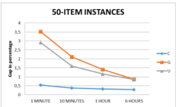
Furthermore, we monitored the percentage gap provided by the solver after one minute, 10 minutes, one hour, and six
hours of computation. The results of these initial tests are summarized in Figure B.1, where we show the gaps in mean
percentage between test instances, grouped by the number of items and type of instances. In particular, C denotes the
original instances of GBPP, G stands for the Gumbel instances of GBPPI, and U represents the uniform instances of
a) Comparisons with 25-item instances b) Comparisons with 50-item instances
c) Comparisons with 100-item instances d) Comparisons with 200-item instances
e) Comparisons with 500-item instances
Figure B.1: Comparisons between the classical GBPP and the new GBPPI. Thex-axis represents time and they-axis gaps in percentage. C denotes classical GBPP instances, G indicates Gumbel-GBPPI instances, and U denotes uniform-GBPPI instances.
From Figure B.1, we can see that the gaps provided by the solver for the GBPPI instances (both Gumbel and uniform) are clearly higher than those of the original GBPP. For example, the gap in mean percentage of the
500-item-GBPP instances is 0.43%, whereas the gap in mean percentage of the corresponding GBPPI instances is 2.50%
for the Gumbel instances and 2.72% for the uniform instances. This suggests that the introduction of the dependence
of item profits on bins involves greater computational effort.
It is worth remarking on the trend in gaps with respect to the range of the minutes. This interval is crucial in
city-logistics settings, where decisions need to be made quickly [51]. It was not possible to report the percentage
gaps for the 500-item instances after one minute of computation because the solver was unable to determine an
initial solution (i.e., the percentage gap was arbitrarily large). The percentage gaps provided by the solver after 10
minutes for the GBPPI instances were acceptable for the 25-item instances only. As the number of items increased
to 50, the gaps increased to 2.12% for Gumbel instances and to 1.60% for uniform instances. The percentage gaps tended to increase as the number of items increased. This trend became considerably more evident for the 500-item
instances, with the GBPP instances having a mean percentage gap of 1.43 and the GBPPI having gaps of 38.19% and
20.57%, respectively, for the Gumbel and uniform instances. These gaps were clearly prohibitive. Moreover, for some
instances the solver was unable to find an initial solution after 10 minutes of computation. All these considerations
indicate that the solver alone is not appropriate to address GBPPI in a city-logistics environment where decisions are