Using and developing declarative languages for machine learning and data mining

(1)

Declarative Languages for Machine

Learning and Data Mining

Luc De Raedt

ICLP, 2015

with slides from

Angelika Kimmig, Davide Nitti, Siegfried Nijssen, Tias Guns, Paolo Frasconi, Francesco Orsini

(2)

Inductive Logic

Programming

•

In 1995 :

•

focus on symbolic data and methods

•

focus on using and producing knowledge

•

learning programs typically written in Prolog

(3)

Inductive Logic

Programming

[Srinivasan et al. AIJ 96]

Data = Set of Small Graphs

General Purpose

Logic Learning System

Uses and Produces

(4)

Learning from entailment

Learning from entailment -- the setting

Given

mutagenic(225), ...

Find

background

examples

rules

covers(H,e) iff H |= e or B

∪

H

⊧

e

(5)

Machine learning and

data mining

•

Today

•

Big data — a lot more data available

•

Low-level and high-level features

•

focus on performance and scalability, less on

understandability

•

kernels, probabilistic methods, constrained

(6)

Declarative methods

•

There has been a paradigm shift in the field of AI from

programming

to

solving

(Hector Geffner at ECAI 2012)

•

Use of solvers and declarative languages is common in AI

•

SAT, MAX-SAT, CSP, ASP, MDPs, ILP, MP, …

•

Two sources of inspiration for this talk

•

Statistical learning (convex optimization) — Stephen Boyd

(7)

Role of Declarative Methods in

ML and DM ?

(8)

ML and DM ?

(9)

Role of Declarative Methods in

ML and DM ?

This talk:

(10)

This talk

•

Using and developing declarative languages for ML/DM — a

survey

•

inductive query languages (database perspective)

•

modelling languages for ML/DM (constraint / answer set

programming)

•

programming languages for ML/DM (programming language

perspective)

•

probabilistic

(11)

(12)

Data Mining

Given

•

a database containing instances or transactions D

•

the set of instances

•

a hypothesis space or pattern language L

•

a selection predicate, query or set of constraints Q

Find Th(Q,L,D) = { h

∈

L | Q(h,D) = true }

(13)

Pattern Mining

Find

patterns that are frequent in mutagenic,

infrequent in clean data.

(14)

Imielinski and Mannila (1995)

The concept of data mining as

a querying process.

•

Make first class citizens of patterns.

•

Query not only the data but also the patterns.

•

Tightly integrate databases and data mining.

•

Search for the equivalent of Codd’s relational algebra for data

mining

“From the user perspective, there is no such thing as a real

discovery, just a matter of

the expressive power of the query

language.”

(15)

An inductive database example

Virtual Mining Views (Blockeel et al. 12)

Beer

Brand

Color

Alcohol%

1

Westmalle Tripel

Blonde

9.5

2

Orval

Dark

6.2

3

Stra

↵

e Hendrik

Gold

9

4

Stra

↵

e Hendrik

Dark

11

....

...

Cid

Brand

Color

Alcohol%

c1

Westmalle Tripel

?

c2

Westmalle Tripel

Blonde

?

c3

?

Blonde

?

c4

?

Blonde

9.5

c5

Stra↵e Hendrik

?

....

...

cid

frequency

size

c5

2

1

...

Beer

Brand

Color

Alcohol%

1

Westmalle Tripel

Blonde

9.5

2

Orval

Dark

6.2

3

Stra

↵

e Hendrik

Gold

9

4

Stra

↵

e Hendrik

Dark

11

(16)

Beer

Brand

Color

Alcohol%

1

Westmalle Tripel

Blonde

9.5

2

Orval

Dark

6.2

3

Stra

↵

e Hendrik

Gold

9

4

Stra

↵

e Hendrik

Dark

11

....

...

Cid

Brand

Color

Alcohol%

c1

Westmalle Tripel

?

c2

Westmalle Tripel

Blonde

?

c3

?

Blonde

?

c4

?

Blonde

9.5

c5

Stra↵e Hendrik

?

....

...

Beer

Brand

Color

Alcohol%

1

Westmalle Tripel

Blonde

9.5

2

Orval

Dark

6.2

3

Stra

↵

e Hendrik

Gold

9

4

Stra

↵

e Hendrik

Dark

11

....

...

Cid

Brand

Color

Alcohol%

c1

Westmalle Tripel

?

c2

Westmalle Tripel

Blonde

?

c3

?

Blonde

?

c4

?

Blonde

9.5

c5

Stra

↵

e Hendrik

?

....

...

cid

frequency

size

c5

2

1

...

(17)

Beer

Brand

Color

Alcohol%

1

Westmalle Tripel

Blonde

9.5

2

Orval

Dark

6.2

3

Stra

↵

e Hendrik

Gold

9

4

Stra

↵

e Hendrik

Dark

11

....

...

Cid

Brand

Color

Alcohol%

c1

Westmalle Tripel

?

c2

Westmalle Tripel

Blonde

?

c3

?

Blonde

?

c4

?

Blonde

9.5

c5

Stra↵e Hendrik

?

....

...

Cid

Brand

Color

Alcohol%

c1

Westmalle Tripel

?

c2

Westmalle Tripel

Blonde

?

c3

?

Blonde

?

c4

?

Blonde

9.5

c5

Stra

↵

e Hendrik

?

....

...

cid

frequency

size

c5

2

1

...

SELECT C.*, S.supp, S.sz,

S.supp * S.sz AS area

FROM BeerConcepts C, BeerSets S

WHERE (C.cid = S.cid AND (S.freq * S.sz > 60))

OR (S.freq > 10)

BeerConcepts

(18)

Understanding city access patterns

•

How do people get into town? What is the

map of their trips in space and time?

Slides courtesy

Dino Pedreschi

(19)

•

How do people get into town? What is the

Slides courtesy

Dino Pedreschi

(20)

A12 Sud

Cascina

Marina di Pisa/Tirrenia Lucca

•

How do people get into town? What is the

Slides courtesy

Dino Pedreschi

(21)

Marina di Pisa/Tirrenia A12 Sud

1,50

%

2,90

%

Slides courtesy

Dino Pedreschi

(22)

M-Atlas kdd.isti.cnr.it

F. Giannotti, M. Nanni, D. Pedreschi, F. Pinelli, C. Renso, S. Rinzivillo, R, Trasarti.

Unveiling the complexity of human mobility by querying and mining massive trajectory data.

VLDB J., 2011

Slides courtesy

Dino Pedreschi

(23)

DMQL EXPRESSIVENESS:

How do people leave the city toward suburban areas?

CREATE MODEL MilanODMatrix AS MINE ODMATRIX FROM (SELECT t.id, t.trajectory FROM TrajectoryTable t), (SELECT orig.id, orig.area FROM MunicipalityTable orig), (SELECT dest.id, dest.area FROM MunicipalityTable dest)

CREATE RELATION CenterToNESuburbTrajectories USING ENTAIL

FROM (SELECT t.id, t.trajectory FROM TrajectoryTable t, MilanODMatrix m WHERE m.origin = Milan AND

m.destination IN (Monza, ..., Brugherio))

CREATE MODEL ClusteringTable AS MINE T-CLUSTERING

FROM (Select t.id, t.trajectory from CenterToNESuburbTrajectories t) SET T-CLUSTERING.FUNCTION = ROUTE_SIMILARITY AND

T-CLUSTERING.EPS = 400 AND T-CLUSTERING.MIN_PTS = 5

M-ATLAS --

Gianotti et al. VLDB J. 11

Mobility mining

(24)

Inductive databases

•

Many inductive query languages have been developed (supporting decision trees,

complex pattern mining, clustering, geographical information systems …), e.g.

MineRule (Meo), MSQL (Iemielinski), DMQL (Han), IQL (Nijssen), LDL ...

•

How does it work :

•

integration in database system + query optimization + specific type of pattern;

•

usually: a call to an external “procedural” solver

•

Challenges :

•

different implementations needed for different pattern types, no “universal”

algebra for data mining known; the quest remains open

•

loose integration among different pattern types, sometimes more a toolbox

•

limited expressiveness (e.g. user-defined constraints absent)

(25)

Constraint-Based Pattern Mining

(26)

Pattern Mining

•

which patterns are frequent ?

•

which patterns are significant w.r.t. classes ? all patterns ? k-best

patterns ?

•

which pattern

set

is the

best

concept-description for the actives ? for

the inactives ?

C. pattern set mining

A. frequent pattern

T h

(

L

, Q,

D

) =

{

p

L|

Q

(

p,

D

) =

true

}

B. Correlated pattern mining = subgroup discovery

T h

(

L

, Q,

D

) = arg

p

L

max

k

(

p,

D

)

(27)

Constraint-Based Mining

•

Numerous constraints have been used

•

Numerous systems have been developed

•

And yet,

•

new constraints often require new

implementations

(28)

Constraint and Answer Set

Programming

•

Exists since about 20 ? years

•

A general and generic methodology for dealing with constraints

across different domains

•

Efficient, extendable general-purpose systems exist, and key

principles have been identified

•

Surprisingly CP & ASP had not been used for data mining ?

•

CP and ASP systems often more elegant, more flexible and

more efficient than special purpose systems

(29)

Itemset mining

Frequent patterns

4

2

3

Data

(30)

(31)

Frequent Itemset Mining

Find

:

all sets of items appearing frequently

cover( , ) = { , }

frequency( , ) = | { , } | = 2

(32)

Given

• I

=

{

1

,

· · ·

, N rI

}

set of items

• T

=

{

1

,

· · ·

, N rT

}

set of transactions

• D

=

{

(

t, I

)

|

t

2

T

, I

✓

I}

dataset

•

Items

✓

I

and

T rans

✓

T

Find

Items

such that

|

covers

(

Items,

D

)

|

> f req

where

covers

(

Items,

D

) =

(33)

int

: Freq;

int

: NrI;

int

: NrT;

array

[1..NrT]

of set of

1..NrI: D;

var set of

1..NrI: Item;

var set of

1..NrT: Trans;

constraint

card(Trans) > Freq;

constraint

Trans = covers(Item, D);

solve satisfy

;

function var set of int: cover(Item, D) =

let {

var set of int: Trans,

constraint forall (t in ub(Trans))

(t in Trans

↔

Item subset D[t]) } in Trans;

int

: Freq;

int

: NrI;

int

: NrT;

array

[1..NrT]

of set of

1..NrI: D;

var set of

1..NrI: Items;

var set of

1..NrT: Trans;

constraint

card(Trans) > Freq;

constraint

Trans = covers(Items, D);

solve satisfy

;

function var set of int: cover(Items, D) =

let {

(t in Trans

↔

Items subset D[t]) } in Trans;

Given

• I

=

{

1

,

· · ·

, N rI

}

set of items

• T

=

{

1

,

· · ·

, N rT

}

set of transactions identifiers

• D

=

{

(

t, I

)

|

t

T

, I

I}

Dataset

•

Items

I

and

T rans

T

Find

Items

such that

|

covers

(

Items,

D

)

|

> f req

where

covers

(

Items,

D

) =

{

t

T |

(

t, I

)

D

and

Items

I

}

MiningZinc [Guns et al IJCAI 13, ICDM 13]

Given

• I

=

{

1

,

· · ·

, N rI

}

set of items

• T

=

{

1

,

· · ·

, N rT

}

set of transactions

• D

=

{

(

t, I

)

|

t

2

T

, I

✓

I}

dataset

•

Items

✓

I

and

T rans

✓

T

Find

Items

such that

|

covers

(

Items,

D

)

|

> f req

where

covers

(

Items,

D

) =

(34)

Declarative Modeling

•

Language goals:

•

high-level notation (similar to paper definitions)

•

solver-independent

•

user-defined abstractions

•

- mathematical-like language (Zinc)

•

- many solvers

•

- can define custom predicates

and functions

[T. Guns, A. Dries, S. Nijssen, G. Tack, L. De Raedt, IJCAI 2013]

(35)

Frequent Itemset Mining

vocabulary FrequentItemsetMiningVoc {

type Transaction

type Item

Freq: int

Includes(Transaction,Item)

FrequentItemset(Item)

}

theory FrequentItemsetMiningTh: FrequentItemsetMiningVoc {

#{t: !i: FrequentItemset(i) => Includes(t,i) } >= Freq.

}

structure Input : FrequentItemsetMiningVoc {

Freq = 7 // threshold for frequent itemsets

Transaction = { t1; ... ; tn } // n transactions

Item = {i1 ; ... ; im } // m items

Includes = {t1,i2; t1,i7; ...} // items of transactions

}

FrequentItemset represents a

set of items

FreqItemset must fulfill

#{t: FreqItemset

⊆

t} >= Freq.

in ASP — See Järvisalo, LPNMR 11

(36)

Closed Itemset Mining

int

: Freq;

int

: NrI;

int

: NrT;

array

[1..NrT]

of set of

1..NrI: D;

var set of

1..NrI: Items;

var set of

1..NrT: Trans;

constraint

card(Trans) > Freq;

constraint

Trans = covers(Items, D);

constraint

Items = cover_inv(Trans, D);

solve satisfy

;

function var set of int: cover(Items, D) =

let {

(t in Trans

↔

Items subset D[t] ) } in Trans;

function var set of int: cover_inv(Trans,D)= let {

var set of int: Items,

constraint forall (i in ub(Items))

(i in Items

↔

Trans subset D’[i] )

} in Items;

(37)

Generality

(38)

Manual Encoding in Zinc

⇤

t

:

T

t

= 1

⇥

i

I

i

(1

D

ti

) = 0

t

T

t

minsup

⇤

i

:

I

i

= 1

⇥

t

T

t

D

ti

minsup

iff

Text

int: Freq;

int: NrI; int: NrT;

array [1..NrT] of set of int: D;

array [1..NrI] of var bool: Items;

array [1..NrT] of var bool: Trans;

constraint % encode D: every Trans complement has no supported Items

forall(t in 1..NrT) (

Trans[t] <-> sum(i in 1..NrI) ( Items[i]*(1 - (i in D[t])) ) <= 0

);

constraint % frequency: every Item is supported by sufficently many Trans

forall(i in 1..NrI) (

Items[i] -> sum(t in 1..NrT) ( Trans[t]*(i in D[t]) ) >= Freq

);

(39)

Resulting Search Strategy akin

to Zaki’s Eclat [KDD 97]

see

(40)

Discriminative Pattern Mining

Alternative opt. functions, for example:

with:

int

: NrI;

int

: NrT;

int

: Freq;

array

[1..NrT]

of set of

int

: D;

set of int

: pos;

set of int

: neg;

var set of

1..NrI: Items;

var set of

1..NrT: Trans;

constraint

Trans = cover(Items, D);

solve maximize

card(Trans

intersect

pos) – card(Trans

intersect

neg

)

neg);

solve maximize

chi2(Trans, pos, neg);

function float

: chi2(Trans, pos, neg)

(41)

Correlation function

Projection on PN-space

Nijssen KDID

(42)

Declarative Modeling

•

Language goals:

•

high-level notation (similar to paper definitions)

•

solver-independent

•

user-defined abstractions

•

- mathematical-like language (Zinc)

•

- many solvers

•

- can define custom predicates

and functions

[T. Guns, A. Dries, S. Nijssen, G. Tack, L. De Raedt, IJCAI 2013]

(43)

Toolchain

1)

Normalize to FlatZinc

(do not flatten lib_itemsetmining.mzn yet)

2)

Apply rewrite rules to:

1)

add redundant constraints

2)

detect (partial) applicability of specialised algorithms

3)

tailor to constraint solvers

3)

Collect all feasible rewrite combinations = execution plans

4)

Heuristically rank + execute a plan

(44)

Three categories of execution plans:

A) Specialised algorithms only

−

Eclat-maxfreq(TDB, 20, 40)

−

LCMv2(TDB, 20) + maxcover(Items, TDB, 40)

B) Hybrid decomposition

−

LCMv2(TDB, 20) + gecode(

card(cover(Items, TDB)) =< 40

)

−

LCMv2(TDB, 20) + frequency(Items, TDB, S) + gecode(

S =< 40

)

C) Generic solvers only

−

gecode(...)

−

gecode-bool(...)

−

gecode-bool(...

+ redundant

)

−

or-tools-bool(...)

var set of

1..NrI: Items;

array

[int]

of set of

int

: TDB;

constraint

card(cover(Items, TDB)) >= 20;

constraint

card(cover(Items, TDB)) =< 40;

(45)

Experiments, hybrid solving

frequent itemset mining, with minimum size and closure constraint

(46)

cis

-regulatory module detection

regulators

Genomic sequences

AGTGAGATAAAAAAAAGTATTGACATGAATTAAAAAACCCAGAAAGCACACTAGGGTGCATCAGTGAGTAGCCTCACAGTCTAAGGGTTTACA GACTTTCTAAACATTCAGA Seq_1 (1,10) (65,74) (12,20) (80,88) (43,51) (53,61) (90,98) (72,78) Seq_2 (33,42) (85,94) (49,57) (56,64) (91,99) (50,56) (52,58) Seq_3 (1,10) (82,91) (45,53) (58,66) (75,83) (90,88) (24,32) (72,80) (89,97)

with CP: add domain-specific

constraints

(47)

Declarative Pattern Mining

•

Quite some work on data mining and CP

•

pattern mining : P. Boizumault, B. Cremilleux, L. De Raedt, T. Guns,

S. Jabbour, M. Jarvisalo, S. Loudni, S. Nijssen, B. O'Sullivan, W.

Ugarte, A. Kemmar, ….

•

clustering : B. Babaki, I. Davidson, T.B.H. Dao, O. du Merle, S.

Gilpin, P. Hansen, S. Nijssen, C. Vrain, …

•

Several papers at CP 15

•

Still many limitations and challenges

•

Expressive power of modeling tools

•

Efficient execution / compilation

(48)

Mining graphs

• Three problems

• subgraph isomorphism — NP-complete subproblem • enumeration of subgraphs

• _{requires lower bound}

• canonical form (do not generate the same graph more than once)

• independent subproblems reusing previous results;

• Some emerging approaches :

• sequences [Negrevergne, CPAIOR 15],[Kemmar, CP 15], • _{graphs : [Paramonov, ILP15]}

(49)

Second-Order Model: Multiple Graphs

Multiple Graph Homomorphism Check:

homo

(

g

)

≈∆ ÷

◊

:

!

bedge

(

x

,

y

)

·

inq

(

x

)

·

inq

(

y

) =

∆

edge

(

g

,

◊

(

x

)

,

◊

(

y

))

.

inq

(

x

)

·

blabel

(

x

) =

y

=

∆

label

(

g

,

◊

(

x

)) =

y

.

x

”

=

y

=

∆

◊

(

x

)

”

=

◊

(

y

)

"

.

Frequency Constraint:

#

{

graph

:

homo

(

graph

)

}

Ø

t

.

13 / 25

Mining graphs

(50)

(51)

Programming Languages for Machine

Learning

(52)

Learning

Probabilistic Programming

(53)

Tom Mitchell

Can we design programming languages containing

machine learning primitives?

Can a new generation of computer programming

languages directly support writing programs that learn?

Why not design a new computer programming language that

supports writing programs in which some subroutines are

hand-coded while others are specified as “to be learned.” Such a

programming language could allow the programmer to declare the

inputs and outputs of each “to be learned” subroutine, then select a

learning algorithm from the primitives provided by the programming

language.

(54)

Tom Mitchell

Can we design programming languages containing

machine learning primitives?

Can a new generation of computer programming

languages directly support writing programs that learn?

Why not design a new computer programming language that

supports writing programs in which some subroutines are

hand-coded while others are specified as “to be learned.” Such a

programming language could allow the programmer

to declare

the

inputs and outputs

of each “to be learned” subroutine,

then select a

learning algorithm

from the primitives provided by the programming

language.

(55)

Probabilistic Prologs

CP-Logic & ProbLog

52

[Vennekens et al, ICLP 04]

throws(john).

0.5::throws(mary).

0.8 :: break :- throws(mary).

0.6 :: break :- throws(john).

probabilistic causal laws

John throws

Window breaks

doesn’t break

Mary throws

doesn’t throw

1.0

0.6

0.4

0.5

0.8

0.2

P(break)=0.6

×

0.5

×

0.8+0.6

×

0.5

×

0.2+0.6

×

0.5+0.4

×

0.5

×

0.8

(56)

Semantics

(

Broken(G)

:

0.3

)

∨

(

Miss

:

0.7

)

←

ThrowAt(G)

.

I

{

M iss

}

Probability tree is an execution model of theory

iff:

•

Each tree-transition

matches

causal law

•

The tree cannot be extended

Each execution model defines the same

probability distribution over final states

Slides CP-logic courtesy Joost Vennekens

I

[

{

M iss

}

I

[

{

Broken

(

G

)

}

•

0

.

3

0

.

7

•

I

|

=

T hrowAt

(

G

)

(57)

Discrete- and continuous-valued random variables

Distributional Clauses (DC)

[Gutmann et al, TPLP 11; Nitti et al, IROS 13]

54

(58)

Distributional Clauses (DC)

length(Obj) ~ gaussian(6.0,0.45) :- type(Obj,glass).

random variable

with Gaussian distribution

54

(59)

stackable(OBot,OTop) :-

≃

length(OBot)

≥

≃

length(OTop),

≃

width(OBot)

≥

≃

width(OTop).

comparing

values of

random variables

54

(60)

Discrete- and continuous-valued random variables

≃

length(OBot)

≥

≃

length(OTop),

≃

width(OBot)

≥

≃

width(OTop).

ontype(Obj,plate) ~ finite([0 : glass, 0.0024 : cup,

0 : pitcher, 0.8676 : plate,

0.0284 : bowl, 0 : serving,

0.1016 : none])

:- obj(Obj), on(Obj,O2), type(O2,plate).

random variable

with

discrete distribution

54

(61)

length(Obj) ~ gaussian(6.0,0.45) :- type(Obj,glass).

≃

length(OBot)

≥

≃

length(OTop),

≃

width(OBot)

≥

≃

width(OTop).

ontype(Obj,plate) ~ finite([0 : glass, 0.0024 : cup,

0 : pitcher, 0.8676 : plate,

0.0284 : bowl, 0 : serving,

0.1016 : none])

:- obj(Obj), on(Obj,O2), type(O2,plate).

54

(62)

•

Defines a generative process (as for CP-logic)

•

Tree can become infinitely wide, so exact inference infeasible and

sampling

needed; likelihood weighting or MCMC …

•

Well-defined under reasonable assumptions; see Gutmann et al., TPLP

11; Nitti et al., IROS 13, ICRA 14;

•

Typical inference tasks :

•

marginal probability of a query P(query)

•

conditional probability P(query | evidence )

(63)

Inference in PLP

•

As in Prolog and logic programming

•

proof

-based, using knowledge compilation

•

As in Answer Set Programming

•

model

based, using knowledge compilation

•

As in Probabilistic Programming

(64)

Learning relational affordances

Learn probabilistic model

From two object interactions

Generalize to N

Shelf

push

Shelf

tap

Shelf

grasp

(65)

Learning relational affordances

Learn probabilistic model

From two object interactions

Generalize to N

Shelf

push

Shelf

tap

Shelf

grasp

(66)

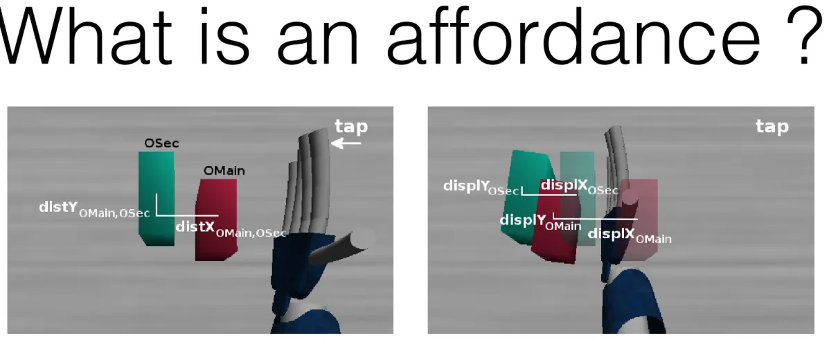
What is an affordance ?

(a) Disparity image (b) Segmented image with landmark points

Clip 7: Illustration of the object size computation. Left-hand image shows the disparity map of the example shown in Figure 5. The orange points in the right-hand image show the points that intersect with the ellipse’s major axis. The orange points are mapped onto 3D using their associated disparity value, and the 3D distance between each pair is defined as the object size.

To learn an a

↵

ordance model, the robot first performs a behavioural babbling

stage, in which it explores the e

↵

ect of its actions on the environment. For

this behavioural babbling stage, for the single-arm actions the robot uses its

right-arm only. For these actions a model of the left-arm will be later built by

exploiting symmetry as in [3]. We include the simultaneous two-arm

push

on

the same object in the babbling phase, allowing for a more accurate modelling

of action e

↵

ects for the iCub.

4

The babbling phase consists of placing pairs of objects in front of the robot

at various positions. The robot executes one of its actions

A

described above on

one object (named: main object,

O

_{M ain}

).

O

_{M ain}

may interact with the other

object (secondary object,

O

Sec

) causing it to also move. Figure 8 shows such

a setting, with the objects’ position before (l) and after (r) a right-arm action

(

tap

(10)) execution.

Clip 8: Relational O before (l), and E after the action execution (r).

4_{As opposed to the two-arm a}_↵_{ordance modelling in [3], we also include in the babbling}

phase the two-arm simultaneous actions whose e↵ects might not always be well modelled by the sum of the individual single-arm actions.

15

•

Formalism — related to STRIPS but models delta

•

but also joint probability model over A, E, O

During this behavioural babbling stage, data for O, A and E are collected for each of the robot’s exploratory actions. The robot executed 150 such exploratory actions. One example of collected data during such an action is shown in Table 1. Note that these values are obtained by the robot from its perception, which naturally introduces uncertainty, which the relational a↵ordance model takes into account (e.g., the displacement of O_{M ain} is observed to be a bit more than 10cm).

Table 1: Example collected O, A, E data for action in Figure 8

Object Properties Action E↵ects

shape_O_{M ain} : sprism shape_O_Sec : sprism distX_O_{M ain}_,O_Sec : 6.94cm

distY_O_{M ain}_,O_Sec : 1.90cm

tap(10)

displX_O_{M ain} : 10.33cm displY_O_{M ain} : 0.68cm

displX_O_Sec : 7.43cm displY_O_Sec : 1.31cm

During the babbling phase, we also learn the action space of each action. As the iCub is not mobile, and each arm has a specific action range, each a_i ₂ A

can be performed when an object is located in a specific action space. An object can be acted upon by both arms, by one arm but not the other, or it can be completely out of the reach of the robot. If the exploratory arm action on an object fails because no inverse kinematics solution was found, then that object is not in that arm’s action space. We will show later how any spatial constraints, such as action space, can be modelled with logical rules.

5.2. Learning the Model

The model will be learnt from the data collected during the robot’s 150 exploratory actions, one instance of such data as illustrated in Table 1. We will model the (relational) object properties: distX, distY (the x and y-axis distance between the centroids of the two objects), and the e↵ects: displX and

displY (the x and y-axis displacement of an object) with continuous distribution random variables. We will start by learning a Linear Conditional Gaussian (LCG) Bayesian Network [26]. An LCG BN specifies a distribution over a mixture of discrete and continuous variables. In an LCG, a discrete random variable may have only discrete parents, while a continuous random variable may have both discrete and continuous parents. A continuous random variable (X) will have a single Gaussian distribution function whose mean depends linearly on the state of its continuous parent variables (Y ) for each configuration of its discrete parent variables (U) [26]. This LCG distribution can be represented as: P(X = x_|Y = y, U = u) = _N(x_|M(u) + W(u)Ty, 2(u)), with M a table of mean values, W a table of regression (weight) coefficient vectors, and a table of variances (independent of Y ). [26]

To learn an LCG BN for our setting, we will approximate displX, displY , and distX and distY by conditional Gaussian distributions over the short dis-tances over which objects interact. These disdis-tances will be enforced by adding logical rules.

(67)

(68)

(69)

(70)

Probabilistic Programs

•

Distributional clauses similar in spirit to probabilistic

functional

languages such as

•

BLOG [Russell et al.], ... but embedded in existing logic and

programming language

•

Church [Goodmann et al.] but use of logic instead of functional

programming ...

•

Probabilistic Logic Programming (survey: De Raedt & Kimmig, MLJ

15):

•

natural

possible world semantics

and link with prob. databases.

•

somewhat harder to do

meta-programming

(71)

Probabilistic Programming

Key idea :

• modeling / programming language

• extend with probabilistic primitives to define probability distribution over possible

worlds or execution traces

• extend with solvers / execution strategies to answer probabilistic queries (marginal,

conditional probabilities, MAP and MPE)

• extend with learning strategies (EM or Bayesian inference) to estimate parameters

and/or learn structure

Many other probabilistic programming languages including

•

PRISM (Sato), Pita (Riguzzi), Blog (Russell), Figaro (Pfeffer), Church

(72)

Learning

Kernel Programming

(73)

Machine learning

Given

•

an unknown target function f: X

→

Y

•

a hypothesis space L containing functions X

→

Y

•

a dataset of examples E = { (x,

f(x)

) | x

∈

X }

•

a loss function loss(h,E)

→

ℝ

(74)

Kernels and SVMs

•

A kernel is a

similarity

measure between two

“observations”, a

dot product

in a feature space

•

Kernels are used by

SVMs

to efficiently compute a

linear separator

65

φ

( )

φ

( )

φ

( )

φ

( )

φ

( )

φ

( )

φ

( )

φ

( )

φ

(.)

φ

( )

φ

( )

φ

( )

φ

( )

φ

( )

φ

( )

φ

( )

φ

( )

φ

( )

φ

( )

Feature space

Input space

k

(

x, x

0

) =

<

(

x

)

,

(

x

0

)

>

(75)

Inductive Logic

Programming

[Srinivasan et al. AIJ 96]

Data = Set of Small Graphs

General Purpose

Logic Learning System

Uses and Produces

(76)

Learning from entailment

Given

mutagenic(225), ...

background

examples

covers(H,e) iff H |= e or B

∪

H

⊧

e

how to define a kernel between relational examples ?

how to do that declaratively ?

(77)

kLOG [Frasconi et al AIJ 14]

Input

Database

Graphicalize

Graphs

Feature

Generation

Graph

Kernel

Feature Vectors

Kernel Matrix

Classifier

Statistical

Learner

(78)

Surgical excision of CNV may allow stabilisation or improvement of vision .

(79)

E/R-MODEL

w depHead next wordID depRel lemma POS-tag chunktag wordString NEGenia NEUMLS sentence hasWord class sentID hasCategory nextS

(80)

s0 s1 s2 s3 next next next s4 s5 s6 s7 s8 s9 title title

Surgical excision of CNV may allow stabilisation or improvement of vision.

background next next dh(nmod) dh(sub) dh(pmod) hasWord

Graphicalization

sentence(s4,4). hasCategory(s4,'background'). w(w4_1,'Surgical','Surgical',b-np,jj,'O','O'). hasWord(s4,w4_1). dh(w4_1,w4_2,nmod). nextW(w4_2,w4_1). w(w4_2,'excision','excision',i-np,nn,'O','O'). hasWord(s4,w4_2). dh(w4_2,w4_5,sub). nextW(w4_3,w4_2). w(w4_3,'of','of',b-pp,in,'O','O'). hasWord(s4,w4_3). dh(w4_3,w4_2,nmod). nextW(w4_4,w4_3). w(w4_4,'CNV','CNV',b-np,nn,'B-protein','O'). hasWord(s4,w4_4). dh(w4_4,w4_3,pmod). nextW(w4_5,w4_4). w(w4_5,'may','may',b-vp,md,'O','O'). hasWord(s4,w4_5). dh(w4_5,w4_0,root). nextW(w4_6,w4_5). ...

(81)

w(Surgical,Surgical,jj,O,O) w4_1 w(excision,excision,nn,O,O) w4_2 w(of,of,in,O,O) w4_3 w(CNV,CNV,nn,B-protein,O) w4_4 w(may,may,md,O,O) w4_5 w(allow,allow,vb,O,O) w4_6 w(stabilisation,stabilisation,nn,O,O) w4_7 w(or,or,cc,O,O) w4_8 w(improvement,improvement,nn,O,O) w4_9 w(of,of,in,O,O) w4_10 w(vision,vision,nn,O,O) w4_11 w(escpoint,escpoint,o,escpoint,O,O) w4_12 dh(nmod) nextW dh(sub) nextW dh(nmod) nextW dh(pmod) nextW dh(root) nextW dh(vc) nextW dh(nmod) nextW dh(nmod) nextW dh(obj) nextW dh(nmod) nextW dh(pmod) nextW dh(p) sentence[4] s4 word(may) hasCategory(background)

distance = 2

...

(82)

radius = 1

distance = 2

...

(83)

radius = 1

distance = 2

...

Extended feature space

(84)

radius = 1

distance = 2

...

Extended feature space

kernel computation ... NSPDK [Costa et al ICML 10]

Propositional learning setting

(85)

Graph Kernels

The decomposition kernel is defined by relations R

r,d

:

k((A,B),(A

′

,B

′

)) = 1 iff (A,B) and (A

′

,B

′

) are pairs of isomorphic

subgraphs — hard match kernel

k((A,B),(A

′

,B

′

)): multinomial distribution of labels in (A,B) or

(A’,B’) — soft match kernel

K(G,G’) =

∑

k((A,B),(A

′

,B

′

)).

A,B: Rr,d-1(A,B,G)

A',B': Rr,d-1(A’,B',G')

r=0 d=0

(86)

(87)

Graph

kernels

domain

representation

machine

learning

prolog facts

&

rules

knowledge base

graph

kernel

. . .

algebraic labels

meta-functions

. . .

learning with

linear separators feature vectors

polynomials

for feature extraction

kProlog

vs

(88)

Tensor operations

76

A

=



1

2

0

3

B

=



2

1

5

1

:- declare(a/2, int).

1::a(0,0).

2::a(0,1).

3::a(1,1).

:- declare(b/2, int).

2::b(0,0).

1::b(0,1).

5::b(1,0).

1::b(1,1).

transpose

A

t

addition

A

+

B

matrix product

AB

c(

I

,

J

a(

J

,

I

).

c(

I

,

J

):- a(

I

,

J

).

c(

I

,

J

):- b(

I

,

J

).

c(

I

,

J

a(

I

,

K

), b(

K

,

J

).

and more…

semi-rings ! cf. Dyna [Eisner]

(89)

sum

L

compress

@

id

dot product

@

dot

some relevant operations

77

kProlog

S

[

x

]

(90)

semiring sum

=

feature addition

78

M

2

⇤

x

_green

+

3

⇤

x

_magenta

2

⇤

x

_sky

+

2

⇤

x

_cyan

+

x

orange

2

⇤

x

_green

+

3

⇤

x

_magenta

+

2

⇤

x

_sky

+

2

⇤

x

_cyan

+

x

orange

kProlog

S

[

x

]

(91)

2

⇤

x

magenta

@id

2

⇤

x

orange

1

⇤

x

cyan

1

⇤

x

magenta

+

1

⇤

x

green

@id

1

⇤

x

magenta

@id

1

⇤

x

sky

2

⇤

x

gray

@id

1

⇤

x

magenta

1

⇤

x

gray

@id

1

⇤

x

green

@id function

=

feature compression

analogous of the

f

function in [Shervashidze et al. (2011)]

79

(92)

1

⇤

x

magenta

+

1

⇤

x

green

2

⇤

x

magenta

@dot

1

x

0

+

1

x

2

= 2

h

P

(

x

)

,

Q

(

x

)

i

=

X

(p

,

e

)

2

P

X

(q

,

e

)

2

Q

pq

@dot

product

example

80

kProlog

S

[

x

]

(93)

L

h

(v

) =

⇢

`(v

)

if

h

= 0

f

(

{L

h

1

(w

)

|

w

2

N

(v

)

}

)

if

h >

0

Recoloring step New colors Recoloring step New colors

Weisfeiler-Lehman algorithm

(a.k.a. color refinement)

Can also be used to initialise GI-testing _algorithms.

(94)

Weisfeiler-Lehman graph kernel

polynomials to represent graph labels 82

WL base

features

WL

feature

| {z } phi(1, graph_a) | {z } " phi(2, graph_a) |{z} " phi(0, graph_a) : declare ( v e r t e x / 2 , polynomial ( i n t ) ) . : declare ( edge asymm / 3 , boolean ) .

: declare ( edge / 3 , polynomial ( i n t ) ) . 1 _⇤ x ( gray ) : : v e r t e x ( graph a , 1 ) .

1 _⇤ x ( gray ) : : v e r t e x ( graph a , 2 ) . 1 _⇤ x ( gray ) : : v e r t e x ( graph a , 3 ) . 1 _⇤ x ( gray ) : : v e r t e x ( graph a , 4 ) . 1 _⇤ x ( gray ) : : v e r t e x ( graph a , 5 ) .

edge asymm ( graph a , 1 , 2 ) . edge asymm ( graph a , 2 , 3 ) . edge asymm ( graph a , 3 , 4 ) . edge asymm ( graph a , 4 , 5 ) .

1 . 0 : : edge ( Graph , A, B):

edge asymm ( Graph , A, B ) . 1 . 0 : : edge ( Graph , A, B):

(95)

polynomials represent multisets of labels @id meta-function for recoloring 83

WL base

features

WL

feature

| {z } phi(1, graph_a) | {z } " phi(2, graph_a) |{z} " phi(0, graph_a) : declare ( w l c o l o r / 3 , polynomial ( i n t ) ) . : declare ( w l c o l o r m u l t i s e t / 3 , polynomial ( i n t ) ) . w l c o l o r m u l t i s e t (H, Graph , V): edge ( Graph , V, W) , w l c o l o r (H, Graph , W) . w l c o l o r ( 0 , Graph , V): v e r t e x ( Graph , V ) . w l c o l o r (H, Graph , V): H > 0 , H1 i s H 1 , @id [ w l c o l o r m u l t i s e t (H1, Graph , V ) ] .

(96)

the base kernel H is the dot product between explicit feature

vector at iteration H

explicit feature vector at iteration H 84

WL base

features

WL

feature

| {z } phi(1, graph_a) | {z } " phi(2, graph_a) |{z} " phi(0, graph_a)

:

declare ( phi / 2 , r e a l ) .

phi (H, Graph):

w l c o l o r (H, Graph , V ) .

:

declare ( base kernel / 3 , r e a l ) .

base kernel (H, Graph , GraphPrime ):

@dot [ phi (H, Graph ) ,

(97)

accumulate base-kernels of successive iterations 85

WL base

features

WL

feature

| {z } phi(1, graph_a) | {z } " phi(2, graph_a) |{z} " phi(0, graph_a) : declare ( k e r n e l w l / 3 , r e a l ) . k e r n e l w l ( 0 , Graph , GraphPrime ):

base kernel ( 0 , Graph , GraphPrime ) .

k e r n e l w l (H, Graph , GraphPrime ):

H > 0 , H1 i s H 1 ,

k e r n e l w l (H1, Graph , GraphPrime ) . k e r n e l w l (H, Graph , GraphPrime ):

H > 0 ,

(98)

kProlog

•

Based on the idea of semi-rings (akin to Dyna

[Eisner] and aProbLog [Kimmig])

•

Combines several semi-rings, employs

meta-functions; semantics based on Tp-operator.

•

Can be used for declarative “kernel programming”

•

[Orsini ILP 15]

(99)

•

Two way interaction

•

Many opportunities for ML/DM

•

expressive power, ease of modeling, solver

independent

•

New challenges for Declarative Methods

•

Many open issues and opportunities for research

…

ML and DM ?

(100)