Forecasting Expected Shortfall: An Extreme Value Approach

(1)

Forecasting Expected Shortfall

An Extreme Value Approach

Benjamin Kjellson

Bachelor’s thesis 2013:K7

Faculty of Science

Centre for Mathematical Sciences

CENTR

UM

SCIENTIAR

UM

MA

THEMA

TICAR

UM

(2)

Abstract

We compare estimates of Value at Risk and Expected Shortfall from AR(1)-GARCH(1,1)-type models (standard GARCH, GJR-GARCH, Component GARCH), to estimates pro-duced using the Peak Over Threshold method on the residuals of these models. We find that the conditional volatility model matters less than the choice of distribution for the in-novations in the loss process, for which we compare the normal and thet-distribution. The Peak Over Threshold estimates are found to improve upon the estimates of the original models, particularly in the case of normally distributed innovations.

(3)

Acknowledgements

I sincerely thank my supervisor Nader Tajvidi for his patience and wise suggestions in my writing of this thesis, and for introducing me to Extreme value theory. I am also thankful for the education that I have received at the Centre for Mathematical Sciences at Lund University, and I express my gratitude to all the inspiring and passionate lecturers I have had during my stay in Lund.

(4)

List of Tables

1 List of data sets tested . . . 26

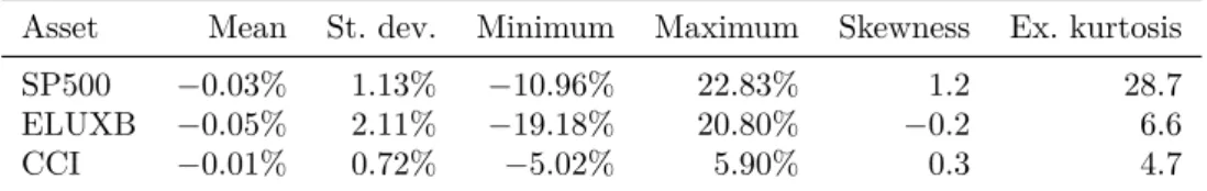
2 Data set Statics. . . 26

3 Parameter Choices . . . 26

4 VaR-breaks . . . 28

5 Unconditional Coverage Test . . . 29

6 Independence Test . . . 30

7 Conditional Coverage Test . . . 31

8 Bootstrap Test for Expected Shortfall . . . 32

9 V1 Test Statistics . . . 33 10 V2 Test Statistics . . . 33 11 V Test Statistics . . . 34

List of Figures

1 S&P 500 Index . . . 4 2 S&P 500 Losses . . . 4

3 S&P 500 Conditional Volatility . . . 5

4 ACF, PACF for Losses of the S&P 500 . . . 5

(a) S&P 500 Losses ACF . . . 5

(b) S&P 500 Losses PACF. . . 5

5 ACF, PACF for the Squared Losses of the S&P 500 . . . 6

(a) S&P 500 Squared Losses ACF . . . 6

(b) S&P 500 Squared Losses PACF . . . 6

6 ACF, PACF for the Squared Residuals . . . 6

(a) S&P 500 Square Residual ACF . . . 6

(b) S&P 500 Square Residual PACF . . . 6

7 Q-Q Plots of Losses and Residuals . . . 7

(a) Q-Q Plot of S&P 500 Losses . . . 7

(b) Q-Q Plot of Residuals . . . 7

8 S&P 500 Value at Risk. . . 31

(6)

1 Introduction

The recent financial crisis illustrated, to some extent, the inadequacy of traditional risk measures such as Value at Risk. Although the current and upcoming regulatory frame-work for supervision and risk management of the banking sector, Basel II and Basel III respectively, still cling to this measure, financial institutions and actors still need proper risk measures for internal use. In this thesis, we consider the risk measure expected short-fall as calculated through variations of the popular AR(1)-GARCH(1,1) model, combined with the Peak Over Threshold model from Extreme value theory to better capture heavy-tail risks. We begin with a short qualitative description of risk management and what the purpose of a risk measure is, what problems are associated with financial data, and how the suggested method for estimating expected shortfall can overcome some of these problems.

1.1 Risk Management, Risk Measures, and Financial Data

Risk management, in its broadest scope, is a systematic approach to identifying, measur-ing, and controlling risks, whatever they may be (Jorion,2001, p. 3). In this thesis though, we limit ourselves to financial risks on the asset level. The most frequently used risk mea-sure for asset or portfolio risk, and indeed the meamea-sure banks and financial institutions must use according to the Basel framework, is Value at Risk (VaR).

VaR is simply a quantile of the loss distribution, telling us, for example, what our worst loss 95 days out of a hundred is expected to be. VaR is thus easy to interpret, and it further lends itself to parametric modelling and backtesting1. However, there are also downsides to VaR as a risk measure, particularly from a mathematical and statistical standpoint. An often-cited paper byArtzner et al. (1999) identifies a few properties that a risk measure ought to have. One of these properties is subadditivity, which for a real valued function f:A →B and elementsa, b∈ A meansf(a+b)≤f(a) +f(b). VaR does not have this property, as the VaR of a portfolio may sometimes be larger than the sum of the VaR for the individual assets in the portfolio (McNeil et al.,2005, p. 40).

An additional downside to VaR is that it does not tell us what the losses look like when VaR is exceeded. An alternative risk measure that solves exactly this problem is expected shortfall (ES), which is the average of the losses beyond a certain quantile of the loss distribution2. That is, ES does not only tell us about the probability of large losses occurring, but also informs us about the likely magnitude of these losses. ES has not only the previously mentioned subadditivity property, but also fulfills the other conditions of a “coherent” risk measure as outlined inArtzner et al.(1999). However, ES also has some downsides which may explain why it is used less often than VaR.Yamai & Yoshiba(2002) showed that the ES measure requires a much larger sample to achieve the same accuracy in backtesting than VaR, which is not strange considering the fact that ES relies on first estimating the VaR, and then adding additional estimates to that. Furthermore, VaR backtests have a much stronger theoretical underpinning than do ES backtests.

1

Testing the measure on historical data without (intentional) look-ahead bias.

(7)

There are a few stylized facts of financial returns that must at least be considered in selecting a risk measure. In this paper, we will pay particular attention to three of these commonly observed phenomena. Volatility clustering is the term used to describe the fact that that large changes in asset prices tend to be followed by further large changes, and that small changes are similarly often followed by small changes (Brooks, 2008, p. 386– 387). A proper risk measure ought then to take account of a sudden spike in volatility in estimating the risk for the following days, and not treat the spike as a one-off event. Another well-known fact is that financial data seem to be generated from distributions with fat tails, meaning that using a normal distribution to model returns may underestimate the frequency of large losses or gains. Therefore, the analytic simplicity of the normal distribution may need to be sacrificed for a distribution or simulation technique that better models reality, so as not to underestimate risks. A third observation about financial data is the so called leverage effect, noted e.g. byBlack(1976). This effect, somewhat improperly named, describes the assymmetry in the influence of past shocks on current volatility, in the sense that a large loss in the past is associated with higher current volatility than is a equally large gain. These three stylized facts form the starting point of this paper.

1.2 Goal

This thesis aims to show how the risk measures Value at Risk and Expected shortfall can be estimated by augmenting variations of the popular AR(1)-GARCH(1,1) model with the Peak Over Threshold model from Extreme value theory. The performance of each model, with or without this augmentation, will be evaluated though backtesting the estimates on a few financial data sets. This will allow for a comparison of the different models. To be specific, the “base” models from time series analysis that we will use will all include an autoregressive component of order one for the return, and the conditional variance models that will be used are

• The GARCH(1,1) model introduced by Bollerslev (1986), which allows us to take into account volatility clustering in our ES estimates.

• The GJR-GARCH(1,1) model by Glosten et al. (1993), which can also account for the leverage effect.

• The Component GARCH(1,1) model ofLee & Engle(1999), in which the conditional variance is decomposed into two parts corresponding to transitory and permanent effects, so that both long-run and short-run movements in volatility are accounted for.

For each such combination of an AR(1) process and a GARCH(1,1) type process, the distribution of the error terms must be decided. For reasons of parsimony, we have used the normal distribution and the Student’s t distribution with four degrees of freedom in estimation—the former to see if it is indeed inadequate and will lead to underestimation of risk, and the latter both of its simplicity in use, and for its fat tails. With these models, we extend the research byMcNeil & Frey(2000), who covered and tested expected shortfall only for the AR(1)-GARCH(1,1) model with normal andt-distributions, and the corresponding POT models fitted to the residuals. In addition, we implement the double bootstrap algorithm by Danielsson et al. (2001) for selection of threshold in the POT models, instead of the more subjective plot-inspection approach byMcNeil & Frey(2000).

(8)

1.3 Caveats

In producing this paper, some choices had to be made that were either somewhat arbitrary or just followed convention when no theoretical basis existed. These choices, and their motivation, include

• Backtesting window length: the length of 1000 observations was chosen because it was the length used in the paper by McNeil & Frey (2000). With about 250 trading days in a year, 1000 observations correspond to around 4 years of data, which admittedly may exclude extreme observations prior to calm stretches of time such as that ending in 2007.

• Data sets: we have chosen to test the models on three data sets, each from a different asset class. More data sets could of course have been included, but there is a trade-off in the amount of time it takes to run a backtest and how much information an additional data set will give us.

• Choice of forecast horizon: we limit ourselves to 1-day forecasts, while multiple-day forecasts may actually be more common in practice. This is again motivated by what the convention seems to be in the articles we have based this paper on.

• Univariate approach: we make our VAR and ES estimates on an asset-by-asset basis rather than on a portfolio of assets, which would be more realistic. For expected shortfall, this can be motivated by the subadditivity property discussed above.

1.4 Previous Research

Value at Risk and Extreme value theory is covered well in most books on risk management and VaR in particular, see for exampleHull(2006),Jorion(2001),McNeil et al.(2005), and Dowd(2005). Vice versa, VaR is treated in some Extreme value theory literature, such as Embrechts et al.(1997) andColes(2001). Expected shortfall is covered in practically every book on risk management as well, although to a much lesser extent than VaR. Instead, we look to the paper byMcNeil & Frey (2000) as inspiration for this thesis; a paper that has generated many follow-up studies, such as those by Byström (2004), Gilli & Këllezi (2006), andTolikas et al.(2007). Newer papers on expected shortfall in combination with conditional volatility models or Extreme value theory often use Bayesian methods; see for example the papers byHoogerheide & van Dijk(2010) andGerlach et al. (2012).

(9)

2 A Look at Some Financial Data

To gain some better intuition about the supposed fat-tailedness and dependence in finan-cial data, we will take a look at one of the data sets used later on. We won’t delve into the theory here—that is done in the next section—but rather just make a few short comments about what we can see. We will have a look at data from the S&P500 index, which is a market cap-weighted index of 500 prominent companies publicly traded in the US stock market. We look at the full data set used for our backtests later on; the models we will use later were decided beforehand, so this poses no problem in terms of a look-ahead bias. We begin by plotting the index series:

400 800 1200 1600 1980 1985 1990 1995 2000 2005 2010 Year Inde x

Figure 1: The S&P 500 index, with data between 1980 and 2011.

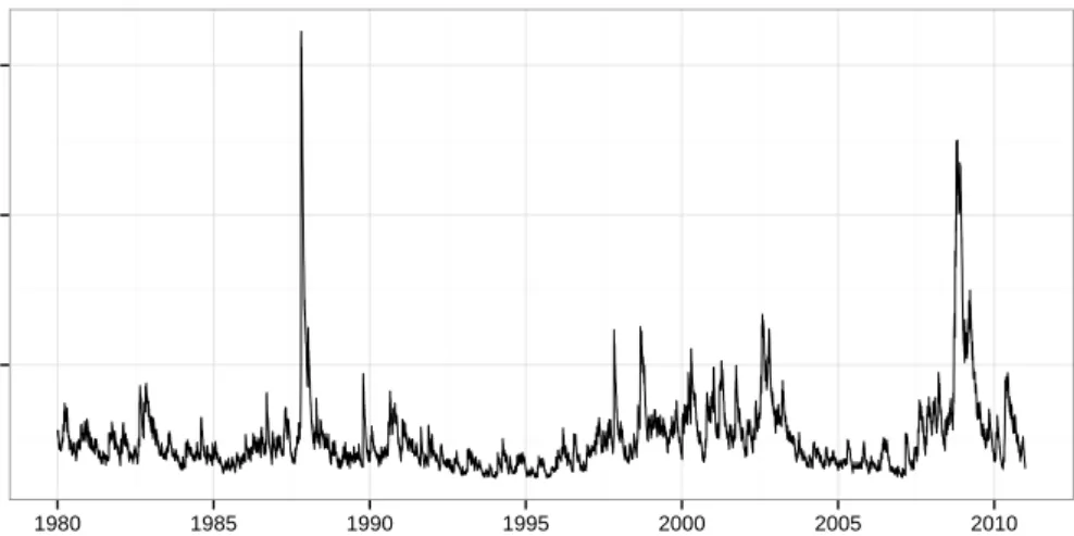
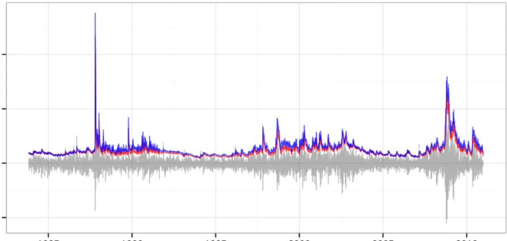
Here we see the long upward trend until the dot-com bubble and the recession in the early 2000s; the recovery in the years after, and then the financial crisis. Next, we look at the losses of the index, keeping an eye out for any trends or clusters in the volatility:

October 19, 1987: Black Monday

−0.1 0.0 0.1 0.2 1980 1985 1990 1995 2000 2005 2010 Year Loss

Figure 2: Losses of the S&P 500 index in the years 1980–2011.

(10)

has been high or low for longer, indicating that it may be dependent on its past. To investigate dependence, we fit one of the models for the losses that we also use later on: an AR(1)-GARCH(1,1) process with normally distributed innovations. Looking at the conditional volatility below, it seems as if there are both short spikes in volatility, and trends that hold for longer.

0.02 0.04 0.06 1980 1985 1990 1995 2000 2005 2010 Year Conditional v olatility

Figure 3: Conditional volatility of the S&P 500, from a fitted AR(1)-GARCH(1,1) model with normally distributed innovations.

To investigate correlations between losses at different times, we take a look at the auto-correlation and partial autoauto-correlation functions for the losses and for the squared losses below. 0.00 0.25 0.50 0.75 1.00 0 5 10 15 20 Lags A CF

(a) ACF for S&P Losses

−0.025 0.000 0.025 0 5 10 15 20 Lags P ar tial A

CF Significant at the_{0.95 level}

False True

(b) PACF for S&P Losses

Figure 4: Autocorrelations and partial autocorrelations for the losses of the S&P 500.

The plot of the ACF indicates a nonexistent or at least low MA order for the losses, while the plot of the PACF indicates a low AR order (assuming the spike at lag 18 is spurious).

(11)

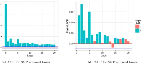
For the squared losses, seen in figure5 below, the dependence is clearer. As the squared returns (or equivalently losses) are usually taken as an approximation of the variance, this indicates that a model in which volatility is allowed to be dependent is suitable for our purposes. 0.00 0.25 0.50 0.75 1.00 0 5 10 15 20 Lags A CF

(a) ACF for S&P squared losses

0.00 0.05 0.10 0.15 0 5 10 15 20 Lags P ar tial A

False True

(b) PACF for S&P squared losses

Figure 5: Autocorrelations and partial autocorrelations for the squared losses of the S&P 500.

It is then interesting to look at the residuals of the fitted AR(1)-GARCH(1,1) model, to see if it has successfully removed dependence in the losses and in the volatility. As the dependence in the losses as they are is already low, we focus on the squares of the residuals, and plot the ACF and PACF for these.

0.00 0.25 0.50 0.75 1.00 0 5 10 15 20 Lags A CF

(a) ACF for the squared residuals

−0.02 −0.01 0.00 0.01 0.02 0 5 10 15 20 Lags P ar tial A

False True

(b) PACF for the squared residuals

Figure 6: Autocorrelations and partial autocorrelations for the squared residuals of the fitted AR(1)-GARCH(1,1) model.

Clearly, the autocorrelation in the squared residuals is smaller than that of the squared losses, which indicates that fitting an AR(1)-GARCH(1,1) model to the data may be a good way of obtaining independent residuals, on which we can then apply methods from

(12)

Extreme value theory to estimate VaR and ES.

To investigate fatness of tails, we can look at Q-Q plots, which show quantiles of the empirical distribution against the theoretical distribution, here chosen to be the normal distribution. We make such plots for both the standardized losses and the standardized residuals of the AR(1)-GARCH(1,1) model, to compare.

●● ● ●●●●● ● ●●●●●●●●●●●●●●●●●●●●●●●●●●●●●●●●●●●●●●●●●●●●●●●●●●●●●●●●●●●●●●●●●●●●●●●●●●●●●●●●●●●●●●●●●●●●●●●●●●●●●●●●●●●●●●●●●●●●●●●●●●●●●●●●●●●●●●●●●●●●●●●●●●●●●●●●●●●●●●●●●●●●●●●●●●●●●●●●●●●●●●●●●●●●●●●●●●●●●●●●●●●●●●●●●●●●●●●●●●●●●●●●●●●●●●●●●●●●●●●●●●●●●●●●●●●●●●●●●●●●●●●●●●●●●●●●●●●●●●●●●●●●●●●●●●●●●●●●●●●●●●●●●●●●●●●●●●●●●●●●●●●●●●●●●●●●●●●●●●●●●●●●●●●●●●●●●●●●●●●●●●●●●●●●●●●●●●●●●●●●●●●●●●●●●●●●●●●●●●●●●●●●●●●●●●●●●●●●●●●●●●●●●●●●●●●●●●●●●●●●●●●●●●●●●●●●●●●●●●●●●●●●●●●●●●●●●●●●●●●●●●●●●●●●●●●●●●●●●●●●●●●●●●●●●●●●●●●●●●●●●●●●●●●●●●●●●●●●●●●●●●●●●●●●●●●●●●●●●●●●●●●●●●●●●●●●●●●●●●●●●●●●●●●●●●●●●●●●●●●●●●●●●●●●●●●●●●●●●●●●●●●●●●●●●●●●●●●●●●●●●●●●●●●●●●●●●●●●●●●●●●●●●●●●●●●●●●●●●●●●●●●●●●●●●●●●●●●●●●●●●●●●●●●●●●●●●●●●●●●●●●●●●●●●●●●●●●●●●●●●●●●●●●●●●●●●●●●●●●●●●●●●●●●●●●●●●●●●●●●●●●●●●●●●●●●●●●●●●●●●●●●●●●●●●●●●●●●●●●●●●●●●●●●●●●●●●●●●●●●●●●●●●●●●●●●●●●●●●●●●●●●●●●●●●●●●●●●●●●●●●●●●●●●●●●●●●●●●●●●●●●●●●●●●●●●●●●●●●●●●●●●●●●●●●●●●●●●●●●●●●●●●●●●●●●●●●●●●●●●●●●●●●●●●●●●●●●●●●●●●●●●●●●●●●●●●●●●●●●●●●●●●●●●●●●●●●●●●●●●●●●●●●●●●●●●●●●●●●●●●●●●●●●●●●●●●●●●●●●●●●●●●●●●●●●●●●●●●●●●●●●●●●●●●●●●●●●●●●●●●●●●●●●●●●●●●●●●●●●●●●●●●●●●●●●●●●●●●●●●●●●●●●●●●●●●●●●●●●●●●●●●●●●●●●●●●●●●●●●●●●●●●●●●●●●●●●●●●●●●●●●●●●●●●●●●●●●●●●●●●●●●●●●●●●●●●●●●●●●●●●●●●●●●●●●●●●●●●●●●●●●●●●●●●●●●●●●●●●●●●●●●●●●●●●●●●●●●●●●●●●●●●●●●●●●●●●●●●●●●●●●●●●●●●●●●●●●●●●●●●●●●●●●●●●●●●●●●●●●●●●●●●●●●●●●●●●●●●●●●●●●●●●●●●●●●●●●●●●●●●●●●●●●●●●●●●●●●●●●●●●●●●●●●●●●●●●●●●●●●●●●●●●●●●●●●●●●●●●●●●●●●●●●●●●●●●●●●●●●●●●●●●●●●●●●●●●●●●●●●●●●●●●●●●●●●●●●●●●●●●●●●●●●●●●●●●●●●●●●●●●●●●●●●●●●●●●●●●●●●●●●●●●●●●●●●●●●●●●●●●●●●●●●●●●●●●●●●●●●●●●●●●●●●●●●●●●●●●●●●●●●●●●●●●●●●●●●●●●●●●●●●●●●●●●●●●●●●●●●●●●●●●●●●●●●●●●●●●●●●●●●●●●●●●●●●●●●●●●●●●●●●●●●●●●●●●●●●●●●●●●●●●●●●●●●●●●●●●●●●●●●●●●●●●●●●●●●●●●●●●●●●●●●●●●●●●●●●●●●●●●●●●●●●●●●●●●●●●●●●●●●●●●●●●●●●●●●●●●●●●●●●●●●●●●●●●●●●●●●●●●●●●●●●●●●●●●●●●●●●●●●●●●●●●●●●●●●●●●●●●●●●●●●●●●●●●●●●●●●●●●●●●●●●●●●●●●●●●●●●●●●●●●●●●●●●●●●●●●●●●●●●●●●●●●●●●●●●●●●●●●●●●●●●●●●●●●●●●●●●●●●●●●●●●●●●●●●●●●●●●●●●●●●●●●●●●●●●●●●●●●●●●●●●●●●●●●●●●●●●●●●●●●●●●●●●●●●●●●●●●●●●●●●●●●●●●●●●●●●●●●●●●●●●●●●●●●●●●●●●●●●●●●●●●●●●●●●●●●●●●●●●●●●●●●●●●●●●●●●●●●●●●●●●●●●●●●●●●●●●●●●●●●●●●●●●●●●●●●●●●●●●●●●●●●●●●●●●●●●●●●●●●●●●●●●●●●●●●●●●●●●●●●●●●●●●●●●●●●●●●●●●●●●●●●●●●●●●●●●●●●●●●●●●●●●●●●●●●●●●●●●●●●●●●●●●●●●●●●●●●●●●●●●●●●●●●●●●●●●●●●●●●●●●●●●●●●●●●●●●●●●●●●●●●●●●●●●●●●●●●●●●●●●●●●●●●●●●●●●●●●●●●●●●●●●●●●●●●●●●●●●●●●●●●●●●●●●●●●●●●●●●●●●●●●●●●●●●●●●●●●●●●●●●●●●●●●●●●●●●●●●●●●●●●●●●●●●●●●●●●●●●●●●●●●●●●●●●●●●●●●●●●●●●●●●●●●●●●●●●●●●●●●●●●●●●●●●●●●●●●●●●●●●●●●●●●●●●●●●●●●●●●●●●●●●●●●●●●●●●●●●●●●●●●●●●●●●●●●●●●●●●●●●●●●●●●●●●●●●●●●●●●●●●●●●●●●●●●●●●●●●●●●●●●●●●●●●●●●●●●●●●●●●●●●●●●●●●●●●●●●●●●●●●●●●●●●●●●●●●●●●●●●●●●●●●●●●●●●●●●●●●●●●●●●●●●●●●●●●●●●●●●●●●●●●●●●●●●●●●●●●●●●●●●●●●●●●●●●●●●●●●●●●●●●●●●●●●●●●●●●●●●●●●●●●●●●●●●●●●●●●●●●●●●●●●●●●●●●●●●●●●●●●●●●●●●●●●●●●●●●●●●●●●●●●●●●●●●●●●●●●●●●●●●●●●●●●●●●●●●●●●●●●●●●●●●●●●●●●●●●●●●●●●●●●●●●●●●●●●●●●●●●●●●●●●●●●●●●●●●●●●●●●●●●●●●●●●●●●●●●●●●●●●●●●●●●●●●●●●●●●●●●●●●●●●●●●●●●●●●●●●●●●●●●●●●●●●●●●●●●●●●●●●●●●●●●●●●●●●●●●●●●●●●●●●●●●●●●●●●●●●●●●●●●●●●●●●●●●●●●●●●●●●●●●●●●●●●●●●●●●●●●●●●●●●●●●●●●●●●●●●●●●●●●●●●●●●●●●●●●●●●●●●●●●●●●●●●●●●●●●●●●●●●●●●●●●●●●●●●●●●●●●●●●●●●●●●●●●●●●●●●●●●●●●●●●●●●●●●●●●●●●●●●●●●●●●●●●●●●●●●●●●●●●●●●●●●●●●●●●●●●●●●●●●●●●●●●●●●●●●●●●●●●●●●●●●●●●●●●●●●●●●●●●●●●●●●●●●●●●●●●●●●●●●●●●●●●●●●●●●●●●●●●●●●●●●●●●●●●●●●●●●●●●●●●●●●●●●●●●●●●●●●●●●●●●●●●●●●●●●●●●●●●●●●●●●●●●●●●●●●●●●●●●●●●●●●●●●●●●●●●●●●●●●●●●●●●●●●●●●●●●●●●●●●●●●●●●●●●●●●●●●●●●●●●●●●●●●●●●●●●●●●●●●●●●●●●●●●●●●●●●●●●●●●●●●●●●●●●●●●●●●●●●●●●●●●●●●●●●●●●●●●●●●●●●●●●●●●●●●●●●●●●●●●●●●●●●●●●●●●●●●●●●●●●●●●●●●●●●●●●●●●●●●●●●●●●●●●●●●●●●●●●●●●●●●●●●●●●●●●●●●●●●●●●●●●●●●●●●●●●●●●●●●●●●●●●●●●●●●●●●●●●●●●●●●●●●●●●●●●●●●●●●●●●●●●●●●●●●●●●●●●●●●●●●●●●●●●●●●●●●●●●●●●●●●●●●●●●●●●●●●●●●●●●●●●●●●●●●●●●●●●●●●●●●●●●●●●●●●●●●●●●●●●●●●●●●●●●●●●●●●●●●●●●●●●●●●●●●●●●●●●●●●●●●●●●●●●●●●●●●●●●●●●●●●●●●●●●●●●●●●●●●●●●●●●●●●●●●●●●●●●●●●●●●●●●●●●●●●●●●●●●●●●●●●●●●●●●●●●●●●●●●●●●●●●●●●●●●●●●●●●●●●●●●●●●●●●●●●●●●●●●●●●●●●●●●●●●●●●●●●●●●●●●●●●●●●●●●●●●●●●●●●●●●●●●●●●●●●●●●●●●●●●●●●●●●●●●●●●●●●●●●●●●●●●●●●●●●●●●●●●●●●●●●●●●●●●●●●●●●●●●●●●●●●●●●●●●●●●●●●●●●●●●●●●●●●●●●●●●●●●●●●●●●●●●●●●●●●●●●●●●●●●●●●●●●●●●●●●●●●●●●●●●●●●●●●●●●●●●●●●●●●●●●●●●●●●●●●●●●●●●●●●●●●●●●●●●●●●●●●●●●●●●●●●●●●●●●●●●●●●●●●●●●●●●●●●●●●●●●●●●●●●●●●●●●●●●●●●●●●●●●●●●●●●●●●●●●●●●●●●●●●●●●●●●●●●●●●●●●●●●●●●●●●●●●●●●●●●●●●●●●●●●●●●●●●●●●●●●●●●●●●●●●●●●●●●●●●●●●●●●●●●●●●●●●●●●●●●●●●●●●●●●●●●●●●●●●●●●●●●●●●●●●●●●●●●●●●●●●●●●●●●●●●●●●●●●●●●●●●●●●●●●●●●●●●●●●●●●●●●●●●●●●●●●●●●●●●●●●●●●●●●●●●●●●●●●●●●●●●●●●●●●●●●●●●●●●●●●●●●●●●●●●●●●●●●●●●●●●●●●●●●●●●●●●●●●●●●●●●●●●●●●●●●●●●●●●●●●●●●●●●●●●●●●●●●●●●●●●●●●●●●●●●●●●●●●●●●●●●●●●●●●●●●●●●●●●●●●●●●●●●●●●●●●●●●●●●●●●●●●●●●●●●●●●●●●●●●●●●●●●●●●●●●●●●●●●●●●●●●●●●●●●●●●●●●●●●●●●●●●●●●●●●●●●●●●●●●●●●●●●●●●●●●●●●●●●●●●●●●●●●●●●●●●●●●●●●●●●●●●●●●●●●●●●●●●●●●●●●●●●●●●●●●●●●●●●●●●●●●●●●●●●●●●●●●●●●●●●●●●●●●●●●●●●●●●●●●●●●●●●●●●●●●●●●●●●●●●●●●●●●●●●●●●●●●●●●●●●●●●●●●●●●●●●●●●●●●●●●●●●●●●●●●●●●●●●●●●●●●●●●●●●●●●●●●●●●●●●●●●●●●●●●●●●●●●●●●●●●●●●●●●●●●●●●●●●●●●●●●●●●●●●●●●●●●●●●●●●●●●●●●●●●●●●●●●●●●●●●●●●●●●●●●●●●●●●●●●●●●●●●●●●●●●●●●●●●●●●●●●●●●●●●●●●●●●●●●●●●●●●●●●●●●●●●●●●●●●●●●●●●●●●●●●●●●●●●●●●●●●●●●●●●●●●●●●●●●●●●●●●●●●●●●●●●●●●●●●●●●●●●●●●●●●●●●●●●●●●●●●●●●●●●●●●●●●●●●●●●●●●●●●●●●●●●●●●●●●●●●●●●●●●●●●●●●●●●●●●●●●●●●●●●●●●●●●●●●●●●●●●●●●●●●●●●●●●●●●●●●●●●●●●●●●●●●●●●●●●●●●●●●●●●●●●●●●●●●●●●●●●●●●●●●●●●●●●●●●●●●●●●●●●●●●●●●●●●●●●●●●●●●●●●●●●●●●●●●●●●●●●●●●●●●●●●●●●●●●●●●●●●●●●●●●●●●●●●●●●●●●●●●●●●●●●●●●●●●●●●●●●●●●●●●●●●●●●●●●●●●●●●●●●●●●●●●●●●●●●●●●●●●●●●●●●●●●●●●●●●●●●●●●●●●●●●●●●●●●●●●●●●●●●●●●●●●●●●●●●●●●●●●●●●●●●●●●●●●●●●●●●●●●●●●●●●●●●●●●●●●●●●●●●●●●●●●●●●●●●●●●●●●●●●●●●●●●●●●●●●●●●●●●●●●●●●●●●●●●●●●●●●●●●●●●●●●●●●●●●●●●●●●●●●●●●●●●●●●●●●●●●●●●●●●●●●●●●●●●●●●●●●●●●●●●●●●●●●●●●●●●●●●●●●●●●●●●●●●●●●●●●●●●●●●●●●●●●●●●●●●●●●●●●●●●●●●●●●●●●●●●●●●●●●●●●●●●●●●●●●●●●●●●●●●●●●●●●●●●●●●●●●●●●●●●●●●●●●●●●●●●●●●●●●●●●●●●●●●●●●●●●●●●●●●●●●●●●●●●●●●●●●●●●●●●●●●●●●●●●●●●●●●●●●●●●●●●●●●●●●●●●●●●●●●●●●●●●●●●●●●●●●●●●●●●●●●●●●●●●●●●●●●●●●●●●●●●●●●●●●●●●●●●●●●●●●●●●●●●●●●●●●●●●●●●●●●●●●●●●●●●●●●●●●●●●●●●●●●●●●●●●●●●●●●●●●●●●●●●●●●●●●●●●●●●●●●●●●●●●●●●●●●●●●●●●●●●●●●●●●●●●●●●●●●●●●●●●●●●●●●●●●●●●●●●●●●●●●●●●●●●●●●●●●●●●●●●●●●●●●●●●●●●●●●●●●●●●●●●●●●●●●●●●●●●●●●●●●●●●●●●●●●●●●●●●●●●●●●●●●●●●●●●●●●●●●●●●●●●●●●●●●●●●●●●●●●●●●●●●●●●●●●●●●●●●●●●●●●●●●●●●●●●●●●●●●●●●●●●●●●●●●●●●●●●●●●●●●●●●●●●●●●●●●●●●●●●●●●●●●●●●●●●●●●●●●●●●●●●●●●●●●●●●●●●●●●●●●●●●●●●●●●●●●●●●●●●●●●●●●●●●●●●●●●●●●●●●●●●●●●●●●●●●●●●●●●●●●●●●●●●●●●●●●●●●●●●●●●●●●●●●●●●●●●●●●●●●●●●●●●●●●●●●●●●●●●●●●●●●●●●●●●●●●●●●●●●●●●●●●●●●●●●●●●●●●●●●●●●●●●●●●●●●●●●●●●●●●●●●●●●●●●●●●●●●●●●●●●●●●●●●●●●●●●●●●●●●●●●●●●●●●●●●●●●●●●●●●●●●●●●●●●●●●●●●●●●●●●●●●●●●●●●●●●●●●●●●●●●●●●●●●●●●●●●●●●●●●●●●●●●●●●●●●●●●●●●●●●●●●●●●●●●●●●●●●●●●●●●●●●●●●●●●●●●●●●●●●●●●●●●●●●●●●●●●●●●●●●●●●●●●●●●●●●●●●●●●●●●●●●●●●●●●●●●●●●●●●●●●●●●●●●●●●●●●●●●●●●●●●●●●●●●●●●●●●●●●●●●●●●●●●●●●●●●●●●●●●●●●●●●●●●●●●●●●●●●●●●●●●●●●●●●●●●●●●●●●●●●●●●●●●●●●●●●●●●●●●●●●●●●●●●●●●●●●●●●●●●●●●●●●●●●●●●●●●●●●●●●●●●●●●●●●●●●●●●●●●●●●●●●●●●●●●●●●●●●●●●●●●●●●●●●●●●●●●●●●●●●●●●●●●●●●●●●●●●●●●●●●●●●●●●●●●●●●●●●●●●●●●●●●●●●●●●●●●●●●●●●●●●●●●●●●●●●●●●●●●●●●●●●●●●●●●●●●●●●●●●●●●●●●●●●●●●●●●●●●●●●●●●●●●●●●●●●●●●●●●●●●●●●●●●●●●●●●●●●●●●●●●●●●●●●●●●●●●●●●●●●●●●●●●●●●●●●●●●●●●●●●●●●●●●●●●●●●●●●●●●●●●●●●●●●●●●●●●●●●●●●●●●●●●●●●●●●●●●●●●●●●●●●●●●●●●●●●●●●●●●●●●●●●●●●●●●●●●●●●●●●●●●●●●●●●●●●●●●●●●●●●●●●●●●●●●●●●●●●●●●●●●●●●●●●●●●●●●●●●●●●●●●●●●●●●●●●●●●●●●●●●●●●●●●●●●●●●●●●●●●●●●●●●●●●●●●●●●●●●●●●●●●●●●●●●●●●●●●●●●●●●●●●●●●●●●●●●●●●●●●●●●●●●●●●●●●●●●●●●●●●●●●●●●●●●●●●●●●●●●●●●●●●●●●●●●●●●●●●●●●●●●●●●●●●●●●●●●●●●●●●●●●●●●●●●●●●●●●●●●●●●●●●●●●●●●●●●●●●●●●●●●●●●●●●●●●●●●●●●●●●●●●●●●●●●●●●●●●●●●●●●●●●●●●●●●●●●●●●●●●●●●●●●●●●●●●●●●●●●●●●●●●●●●●●●●●●●●●●●●●●●●●●●●●●●●●●●●●●●●●●●●●●●●●●●●●●●●●●●●●●●●●●●●●●●●●●●●●●●●●●●●●●●●●●●●●●●●●●●●●●●●●●●●●●●●●●●●●●●●●●●●●●●●●●●●●●●●●●●●●●●●●●●●●●●●●●●●●●●●●●●●●●●●●●●●●●●●●●●●●●●●●●●●●●●●●●●●●●●●●●●●●●●●●●●●●●●●●●●●●●●●●●●●●●●●●●●●●●●●●●●●●●●●●●●●●●●●●●●●●●●●●●●●●●●●●●●●●●●●●●●●●●●●●●● ●● ●●● ● −10 0 10 20 −4 −2 0 2 4 Theoretical Quantiles Sample Quantiles Standardized Losses

(a) Q-Q plot of S&P 500 losses

● ●●● ●●●●●●●●●●●●●●●●●●●●●●●●●●●●●●●●●●●●●●●●●●●●●●●●●●●●●●●●●●●●●●●●●●●●●●●●●●●●●●●●●●●●●●●●●●●●●●●●●●●●●●●●●●●●●●●●●●●●●●●●●●●●●●●●●●●●●●●●●●●●●●●●●●●●●●●●●●●●●●●●●●●●●●●●●●●●●●●●●●●●●●●●●●●●●●●●●●●●●●●●●●●●●●●●●●●●●●●●●●●●●●●●●●●●●●●●●●●●●●●●●●●●●●●●●●●●●●●●●●●●●●●●●●●●●●●●●●●●●●●●●●●●●●●●●●●●●●●●●●●●●●●●●●●●●●●●●●●●●●●●●●●●●●●●●●●●●●●●●●●●●●●●●●●●●●●●●●●●●●●●●●●●●●●●●●●●●●●●●●●●●●●●●●●●●●●●●●●●●●●●●●●●●●●●●●●●●●●●●●●●●●●●●●●●●●●●●●●●●●●●●●●●●●●●●●●●●●●●●●●●●●●●●●●●●●●●●●●●●●●●●●●●●●●●●●●●●●●●●●●●●●●●●●●●●●●●●●●●●●●●●●●●●●●●●●●●●●●●●●●●●●●●●●●●●●●●●●●●●●●●●●●●●●●●●●●●●●●●●●●●●●●●●●●●●●●●●●●●●●●●●●●●●●●●●●●●●●●●●●●●●●●●●●●●●●●●●●●●●●●●●●●●●●●●●●●●●●●●●●●●●●●●●●●●●●●●●●●●●●●●●●●●●●●●●●●●●●●●●●●●●●●●●●●●●●●●●●●●●●●●●●●●●●●●●●●●●●●●●●●●●●●●●●●●●●●●●●●●●●●●●●●●●●●●●●●●●●●●●●●●●●●●●●●●●●●●●●●●●●●●●●●●●●●●●●●●●●●●●●●●●●●●●●●●●●●●●●●●●●●●●●●●●●●●●●●●●●●●●●●●●●●●●●●●●●●●●●●●●●●●●●●●●●●●●●●●●●●●●●●●●●●●●●●●●●●●●●●●●●●●●●●●●●●●●●●●●●●●●●●●●●●●●●●●●●●●●●●●●●●●●●●●●●●●●●●●●●●●●●●●●●●●●●●●●●●●●●●●●●●●●●●●●●●●●●●●●●●●●●●●●●●●●●●●●●●●●●●●●●●●●●●●●●●●●●●●●●●●●●●●●●●●●●●●●●●●●●●●●●●●●●●●●●●●●●●●●●●●●●●●●●●●●●●●●●●●●●●●●●●●●●●●●●●●●●●●●●●●●●●●●●●●●●●●●●●●●●●●●●●●●●●●●●●●●●●●●●●●●●●●●●●●●●●●●●●●●●●●●●●●●●●●●●●●●●●●●●●●●●●●●●●●●●●●●●●●●●●●●●●●●●●●●●●●●●●●●●●●●●●●●●●●●●●●●●●●●●●●●●●●●●●●●●●●●●●●●●●●●●●●●●●●●●●●●●●●●●●●●●●●●●●●●●●●●●●●●●●●●●●●●●●●●●●●●●●●●●●●●●●●●●●●●●●●●●●●●●●●●●●●●●●●●●●●●●●●●●●●●●●●●●●●●●●●●●●●●●●●●●●●●●●●●●●●●●●●●●●●●●●●●●●●●●●●●●●●●●●●●●●●●●●●●●●●●●●●●●●●●●●●●●●●●●●●●●●●●●●●●●●●●●●●●●●●●●●●●●●●●●●●●●●●●●●●●●●●●●●●●●●●●●●●●●●●●●●●●●●●●●●●●●●●●●●●●●●●●●●●●●●●●●●●●●●●●●●●●●●●●●●●●●●●●●●●●●●●●●●●●●●●●●●●●●●●●●●●●●●●●●●●●●●●●●●●●●●●●●●●●●●●●●●●●●●●●●●●●●●●●●●●●●●●●●●●●●●●●●●●●●●●●●●●●●●●●●●●●●●●●●●●●●●●●●●●●●●●●●●●●●●●●●●●●●●●●●●●●●●●●●●●●●●●●●●●●●●●●●●●●●●●●●●●●●●●●●●●●●●●●●●●●●●●●●●●●●●●●●●●●●●●●●●●●●●●●●●●●●●●●●●●●●●●●●●●●●●●●●●●●●●●●●●●●●●●●●●●●●●●●●●●●●●●●●●●●●●●●●●●●●●●●●●●●●●●●●●●●●●●●●●●●●●●●●●●●●●●●●●●●●●●●●●●●●●●●●●●●●●●●●●●●●●●●●●●●●●●●●●●●●●●●●●●●●●●●●●●●●●●●●●●●●●●●●●●●●●●●●●●●●●●●●●●●●●●●●●●●●●●●●●●●●●●●●●●●●●●●●●●●●●●●●●●●●●●●●●●●●●●●●●●●●●●●●●●●●●●●●●●●●●●●●●●●●●●●●●●●●●●●●●●●●●●●●●●●●●●●●●●●●●●●●●●●●●●●●●●●●●●●●●●●●●●●●●●●●●●●●●●●●●●●●●●●●●●●●●●●●●●●●●●●●●●●●●●●●●●●●●●●●●●●●●●●●●●●●●●●●●●●●●●●●●●●●●●●●●●●●●●●●●●●●●●●●●●●●●●●●●●●●●●●●●●●●●●●●●●●●●●●●●●●●●●●●●●●●●●●●●●●●●●●●●●●●●●●●●●●●●●●●●●●●●●●●●●●●●●●●●●●●●●●●●●●●●●●●●●●●●●●●●●●●●●●●●●●●●●●●●●●●●●●●●●●●●●●●●●●●●●●●●●●●●●●●●●●●●●●●●●●●●●●●●●●●●●●●●●●●●●●●●●●●●●●●●●●●●●●●●●●●●●●●●●●●●●●●●●●●●●●●●●●●●●●●●●●●●●●●●●●●●●●●●●●●●●●●●●●●●●●●●●●●●●●●●●●●●●●●●●●●●●●●●●●●●●●●●●●●●●●●●●●●●●●●●●●●●●●●●●●●●●●●●●●●●●●●●●●●●●●●●●●●●●●●●●●●●●●●●●●●●●●●●●●●●●●●●●●●●●●●●●●●●●●●●●●●●●●●●●●●●●●●●●●●●●●●●●●●●●●●●●●●●●●●●●●●●●●●●●●●●●●●●●●●●●●●●●●●●●●●●●●●●●●●●●●●●●●●●●●●●●●●●●●●●●●●●●●●●●●●●●●●●●●●●●●●●●●●●●●●●●●●●●●●●●●●●●●●●●●●●●●●●●●●●●●●●●●●●●●●●●●●●●●●●●●●●●●●●●●●●●●●●●●●●●●●●●●●●●●●●●●●●●●●●●●●●●●●●●●●●●●●●●●●●●●●●●●●●●●●●●●●●●●●●●●●●●●●●●●●●●●●●●●●●●●●●●●●●●●●●●●●●●●●●●●●●●●●●●●●●●●●●●●●●●●●●●●●●●●●●●●●●●●●●●●●●●●●●●●●●●●●●●●●●●●●●●●●●●●●●●●●●●●●●●●●●●●●●●●●●●●●●●●●●●●●●●●●●●●●●●●●●●●●●●●●●●●●●●●●●●●●●●●●●●●●●●●●●●●●●●●●●●●●●●●●●●●●●●●●●●●●●●●●●●●●●●●●●●●●●●●●●●●●●●●●●●●●●●●●●●●●●●●●●●●●●●●●●●●●●●●●●●●●●●●●●●●●●●●●●●●●●●●●●●●●●●●●●●●●●●●●●●●●●●●●●●●●●●●●●●●●●●●●●●●●●●●●●●●●●●●●●●●●●●●●●●●●●●●●●●●●●●●●●●●●●●●●●●●●●●●●●●●●●●●●●●●●●●●●●●●●●●●●●●●●●●●●●●●●●●●●●●●●●●●●●●●●●●●●●●●●●●●●●●●●●●●●●●●●●●●●●●●●●●●●●●●●●●●●●●●●●●●●●●●●●●●●●●●●●●●●●●●●●●●●●●●●●●●●●●●●●●●●●●●●●●●●●●●●●●●●●●●●●●●●●●●●●●●●●●●●●●●●●●●●●●●●●●●●●●●●●●●●●●●●●●●●●●●●●●●●●●●●●●●●●●●●●●●●●●●●●●●●●●●●●●●●●●●●●●●●●●●●●●●●●●●●●●●●●●●●●●●●●●●●●●●●●●●●●●●●●●●●●●●●●●●●●●●●●●●●●●●●●●●●●●●●●●●●●●●●●●●●●●●●●●●●●●●●●●●●●●●●●●●●●●●●●●●●●●●●●●●●●●●●●●●●●●●●●●●●●●●●●●●●●●●●●●●●●●●●●●●●●●●●●●●●●●●●●●●●●●●●●●●●●●●●●●●●●●●●●●●●●●●●●●●●●●●●●●●●●●●●●●●●●●●●●●●●●●●●●●●●●●●●●●●●●●●●●●●●●●●●●●●●●●●●●●●●●●●●●●●●●●●●●●●●●●●●●●●●●●●●●●●●●●●●●●●●●●●●●●●●●●●●●●●●●●●●●●●●●●●●●●●●●●●●●●●●●●●●●●●●●●●●●●●●●●●●●●●●●●●●●●●●●●●●●●●●●●●●●●●●●●●●●●●●●●●●●●●●●●●●●●●●●●●●●●●●●●●●●●●●●●●●●●●●●●●●●●●●●●●●●●●●●●●●●●●●●●●●●●●●●●●●●●●●●●●●●●●●●●●●●●●●●●●●●●●●●●●●●●●●●●●●●●●●●●●●●●●●●●●●●●●●●●●●●●●●●●●●●●●●●●●●●●●●●●●●●●●●●●●●●●●●●●●●●●●●●●●●●●●●●●●●●●●●●●●●●●●●●●●●●●●●●●●●●●●●●●●●●●●●●●●●●●●●●●●●●●●●●●●●●●●●●●●●●●●●●●●●●●●●●●●●●●●●●●●●●●●●●●●●●●●●●●●●●●●●●●●●●●●●●●●●●●●●●●●●●●●●●●●●●●●●●●●●●●●●●●●●●●●●●●●●●●●●●●●●●●●●●●●●●●●●●●●●●●●●●●●●●●●●●●●●●●●●●●●●●●●●●●●●●●●●●●●●●●●●●●●●●●●●●●●●●●●●●●●●●●●●●●●●●●●●●●●●●●●●●●●●●●●●●●●●●●●●●●●●●●●●●●●●●●●●●●●●●●●●●●●●●●●●●●●●●●●●●●●●●●●●●●●●●●●●●●●●●●●●●●●●●●●●●●●●●●●●●●●●●●●●●●●●●●●●●●●●●●●●●●●●●●●●●●●●●●●●●●●●●●●●●●●●●●●●●●●●●●●●●●●●●●●●●●●●●●●●●●●●●●●●●●●●●●●●●●●●●●●●●●●●●●●●●●●●●●●●●●●●●●●●●●●●●●●●●●●●●●●●●●●●●●●●●●●●●●●●●●●●●●●●●●●●●●●●●●●●●●●●●●●●●●●●●●●●●●●●●●●●●●●●●●●●●●●●●●●●●●●●●●●●●●●●●●●●●●●●●●●●●●●●●●●●●●●●●●●●●●●●●●●●●●●●●●●●●●●●●●●●●●●●●●●●●●●●●●●●●●●●●●●●●●●●●●●●●●●●●●●●●●●●●●●●●●●●●●●●●●●●●●●●●●●●●●●●●●●●●●●●●●●●●●●●●●●●●●●●●●●●●●●●●●●●●●●●●●●●●●●●●●●●●●●●●●●●●●●●●●●●●●●●●●●●●●●●●●●●●●●●●●●●●●●●●●●●●●●●●●●●●●●●●●●●●●●●●●●●●●●●●●●●●●●●●●●●●●●●●●●●●●●●●●●●●●●●●●●●●●●●●●●●●●●●●●●●●●●●●●●●●●●●●●●●●●●●●●●●●●●●●●●●●●●●●●●●●●●●●●●●●●●●●●●●●●●●●●●●●●●●●●●●●●●●●●●●●●●●●●●●●●●●●●●●●●●●●●●●●●●●●●●●●●●●●●●●●●●●●●●●●●●●●●●●●●●●●●●●●●●●●●●●●●●●●●●●●●●●●●●●●●●●●●●●●●●●●●●●●●●●●●●●●●●●●●●●●●●●●●●●●●●●●●●●●●●●●●●●●●●●●●●●●●●●●●●●●●●●●●●●●●●●●●●●●●●●●●●●●●●●●●●●●●●●●●●●●●●●●●●●●●●●●●●●●●●●●●●●●●●●●●●●●●●●●●●●●●●●●●●●●●●●●●●●●●●●●●●●●●●●●●●●●●●●●●●●●●●●●●●●●●●●●●●●●●●●●●●●●●●●●●●●●●●●●●●●●●●●●●●●●●●●●●●●●●●●●●●●●●●●●●●●●●●●●●●●●●●●●●●●●●●●●●●●●●●●●●●●●●●●●●●●●●●●●●●●●●●●●●●●●●●●●●●●●●●●●●●●●●●●●●●●●●●●●●●●●●●●●●●●●●●●●●●●●●●●●●●●●●●●●●●●●●●●●●●●●●●●●●●●●●●●●●●●●●●●●●●●●●●●●●●●●●●●●●●●●●●●●●●●●●●●●●●●●●●●●●●●●●●●●●●●●●●●●●●●●●●●●●●●●●●●●●●●●●●●●●●●●●●●●●●●●●●●●●●●●●●●●●●●●●●●●●●●●●●●●●●●●●●●●●●●●●●●●●●●●●●●●●●●●●●●●●●●●●●●●●●●●●●●●●●●●●●●●●●●●●●●●●●●●●●●●●●●●●●●●●●●●●●●●●●●●●●●●●●●●●●●●●●●●●●●●●●●●●●●●●●●●●●●●●●●●●●●●●●●●●●●●●●●●●●●●●●●●●●●●●●●●●●●●●●●●●●●●●●●●●●●●●●●●●●●●●●●●●●●●●●●●●●●●●●●●●●●●●●●●●●●●●●●●●●●●●●●●●●●●●●●●●●●●●●●●●●●●●●●●●●●●●●●●●●●●●●●●●●●●●●●●●●●●●●●●●●●●●●●●●●●●●●●●●●●●●●●●●●●●●●●●●●●●●●●●●●●●●●●●●●●●●●●●●●●●●●●●●●●●●●●●●●●●●●●●●●●●●●●●●●●●●●●●●●●●●●●●●●●●●●●●●●●●●●●●●●●●●●●●●●●●●●●●●●●●●●●●●●●●●●●●●●●●●●●●●●●●●●●●●●●●●●●●●●●●●●●●●●●●●●●●●●●●●●●●●●●●●●●●●●●●●●●●●●●●●●●●●●●●●●●●●●●●●●●●●●●●●●●●●●●●●●●●●●●●●●●●●●●●●●●●●●●●●●●●●●●●●●●●●●●●●●●●●●●●●●●●●●●●●●●●●●●●●●●●●●●●●●●●●●●●●●●●●●●●●●●●●●●●●●●●●●●●●●●●●●●●●●●●●●●●●●●●●●●●●●●●●●●●●●●●●●●●●●●●●●●●●●●●●●●●●●●●●●●●●●●●●●●●●●●●●●●●●●●●●●●●●●●●●●●●●●●●●●●●●●●●●●●●●●●●●●●●●●●●●●●●●●●●●●●●●●●●●●●●●●●●●●●●●●●●●●●●●●●●●●●●●●●●●●●●●●●●●●●●●●●●●●●●●●●●●●●●●●●●●●●●●●●●●●●●●●●●●●●●●●●●●●●●●●●●●●●●●●●●●●●●●●●●●●●●●●●●●●●●●●●●●●●●●●●●●●●●●●●●●●●●●●●●●●●●●●●●●●●●●●●●●●●●●●●●●●●●●●●●●●●●●●●●●●●●●●●●●●●●●●●●●●●●●●●●●●●●●●●●●●●●●●●●●●●●●●●●●●●●●●●●●●●●●●●●●●●●●●●●●●●●●●●●●●●●●●●●●●●●●●●●●●●●●●●●●●●●●●●●●●●●●●●●●●●●●●●●●●●●●●●●●●●●●●●●●●●●●●●●●●●●●●●●●●●●●●●●●●●●●●●●●●●●●●●●●●●●●●●●●●●●●●●●●●●●●●●●●●●●●●●●●●●●●●●●●●●●●●●●●●●●●●●●●●●●●●●●●●●●●●●●●●●●●●●●●●●●●●●●●●●●●●●●●●●●●●●●●●●●●●●●●●●●●●●●●●●●●●●●●●●●●●●●●●●●●●●●●●●●●●●●●●●●●●●●●●●●●●●●●●●●●●●●●●●●●●●●●●●●●●●●●●●●●●●●●●●●●●●●●●●●●●●●●●●●●●●●●●●●●●●●●●●●●●●●●●●●●●●●●●●●●●●●●●●●●●●●●●●●●●●●●●●●●●●●●●●●●●●●●●●●●●●●●●●●●●●●●●●●●●●●●●●●●●●●●●●●●●●●●●●●●●●●●●●●●●●●●●●●●●●●●●●●●●●●●●●●●●●●●●●●●●●●●●●●●●●●●●●●●●●●●●●●●●●●●●●●●●●●●●●●●●●●●●●●●●●●●●●●●●●●●●●●●●●●●●●●●●●●●●●●●●●●●●●●●●●●●●●●●●●●●●●●●●●●●●●●●●●●●●●●●●●●●●●●●●●●●●●●●●●●●●●●●●●●●●●●●●●●●●●●●●●●●●●●●●●●●●●●●●●●●●●●●●●●●●●●●●●●●●●●●●●●●●●●●●●●●●●●●●●●●●●●●●●●●●●●●●●●●●●●●●●●●●●●●●●●●●●●●●●●●●●●●●●●●●●●●●●●●●●●●●●●●●●●●●●●●●●●●●●●●●●●●●●●●●●●●●●●●●●●●●●●●●●●●●●●●●●●●●●●●●●●●●●●●●●●●●●●●●●●●●●●●●●●●●●●●●●●●●●●●●●●●●●●●●●●●●●●●●●●●●●●●●●●●●●●●●●●●●●●●●●●●●●●●●●●●●●●●●●●●●●●●●●●●●●●●●●●●●●●●●●●●●●●●●●●●●●●●●●●●●●●●●●●●●●●●●●●●●●●●●●●●●●●●●●●●●●●●●●●●●●●●●●●●●●●●●●●●●●●●●●●●●●●●●●●●●●●●●●●●●●●●●●●●●●●●●●●●●●●●●●●●●●●●●●●●●●●●●●●●●●●●●●●●●●●●●●●●●●●●●●●●●●●●●●●●●●●●●●●●●●●●●●●●●●●●●●●●●●●●●●●●●●●●●●●●●●●●●●●●●●●●●●●●●●●●●●●●●●●●●●●●●●●●●●●●●●●●●●●●●●●●●●●●●●●●●●●●●●●●●●●●●●●● ●●● ● ●● ● ● −5 0 5 10 −4 −2 0 2 4 Theoretical Quantiles Sample Quantiles Standardized Residuals (b) Q-Q plot of residuals

Figure 7: Q-Q plots for the standardized losses and the standardized residuals of the fitted AR(1)-GARCH(1,1) model, for the S&P 500.

As seen in the Q-Q plots above, the data shows signs of fatter tails than what would be the case had losses been normally distributed. Even though the conditional model makes the situation slightly better, the signs of fat tails are still evident. This speaks for fitting a Generalized Pareto distribution to the tails, in order to estimate value at risk and expected shortfall more accurately.

(13)

3 Theoretical Background

In this section, we present the mathematical details of the risk measures and models mentioned. The aim is to give an outline of the theory behind our estimator for expected shortfall, without delving too deep into the general theories. Before we begin, we take a moment to define the variables we will be working with, namely the return and losses on financial assets.

3.1 Asset Returns and Losses

Denoting bySt,t∈Z, the closing price of an asset at dayt, the raw returns for dayt+ 1

are defined by St+1−St St = St+1 St −1 (3.1)

Since log(1 +x)≈x for x close to zero, and since one-day returns are usually small, the one-day raw returns can be approximated by the one-day log returns, which are defined as Rt+1= log _S t+1 St = log(St+1)−log(St) (3.2)

We then define the loss Xt at day tas the negative of the log-return, i.e. Xt =−Rt. As

we are interested in future returns and future losses, we consider these to be (continuous) random variables. We treat losses as positive numbers rather than negative ones out of convenience; for example, most literature on extreme value theory deals with the upper tails of distributions, although the results apply equally well to the lower tails (through a simple transformation). We will be working with losses in this form throughout the paper, as opposed to measuring losses in money amounts (of a fictitious portfolio, or something similar).

As a basis for all models we test in this paper, we will assume that the losses{Xt,t∈Z},

form a stationary time series where

Xt=µt+σtZt (3.3)

where{Zt} are iid (independent and identically distributed) continuous random variables

with mean zero, unit variance, and come from a location-scale family, and where µt and

(14)

3.2 Value at Risk

The value at risk for a given confidence levelq∈(0,1) and timetis given by the smallest numberxq such that the lossXt+1 at timet+ 1 will fall belowxq with probabilityq:

VaRt_q= inf{xq∈R:P(Xt+1 ≤xq)≥q}= inf{xq∈R:P(Xt+1 > xq)≤1−q} (3.4)

Thus, value at risk is a quantile of the loss distribution, andqis usually taken to be in the range [0.9,1), so that we may talk about the “95%-VaR” or “99%-VaR”. Sometimes, the

coverage rateα= 1−q is used instead. Note that the above is just the one-day VaR; the concept can be extended to longer horizons of five days, ten days, or more. This can be done in several ways; a common way for shorter horizons is to simply multiply the 1-day estimate of VAR by the square root of the number of days ahead one wishes to forecast; this is the so-called square-root-of-time rule. See McNeil et al. (2005, p. 54) for more details.

With some improper functional notation, if the random variableZ is normally distributed with meanµ and varianceσ2, then forq ∈(0,1) the VaR ofZ is given by

VaR_q(Z) =µ+σΦ−1(q) (3.5)

where Φ is the cumulative distribution function of a standard normal variable (McNeil et al.,2005, p. 39).

If instead the normalized random variable ˜Z = Z−µ_σ has a standard t-distribution with ν >2 degrees of freedom, so that E( ˜Z) = 0 and Var( ˜Z) = _ν−ν₂, then the VaR ofZ is given by

VaR_q(Z) =µ+σ t−_ν1(q) (3.6) wheretν denotes the distribution function of the standard Student’st-distribution (McNeil

et al.,2005, p. 40).

As these two examples allude to, similar results can be obtained from any location-scale family of distributions (McNeil et al.,2005, p. 40).

For losses the type of losses we are considering (see equation (3.3)), where the mean and variance are possibly time-dependent but the innovations are not, we may write VaRt_q(Xt+1) = µt+1 +σt+1 ·VaRq(Z) for the value at risk at time t for the loss at time

t+ 1.

(15)

3.3 Expected Shortfall

The expected shortfall at levelq, in turn, is the expected value at timetof the loss in the next period,Xt+1, conditional on the loss exceeding VaRtq:

ESt_q = Et[Xt+1|Xt+1>VaRq] (3.7)

For this reason, expected shortfall is also referred to as Expected Tail Loss or Conditional VaR. Just as for VaR, expected shortfall can also be estimated over longer horizons than a day, and again the square-root-of-time rule can be used.

For q ∈ (0,1), the expected shortfall for a normally distributed random variable Z with meanµ and varianceσ2 is

ESq(Z) =µ+σ

φ(Φ−1(q))

1−q (3.8)

whereφis the density of a standard normal variable (McNeil et al.,2005, p. 45).

If instead the random variable ˜Z = Z−µ_σ has a standardt-distribution with ν >2 degrees of freedom, then the expected shortfall ofZ is given by

ESq(Z) =µ+σ gν t−ν1(q) 1−q · ν+ t−_ν1(q)2 ν−1 (3.9)

wheregν denotes the density of the standard Student’s t-distribution (McNeil et al.,2005,

p. 45–46).

Analogous to the VaR calculations, the calculation of expected shortfall will be similar for any random variable from a location-scale family. Thus, for the losses that we are considering (see equation (3.3)), where the mean and variance are possibly time-dependent but the innovations Z are not, we may write ESt_q(Xt+1) =µt+1+σt+1·ESq(Z). This is

the expected shortfall at timet for the loss at timet+ 1.

(16)

3.4 Time Series

In this section we establish some properties of certain stochastic processes, that we will use to model the asset returns (or losses).

Consider a discrete time stochastic process {Xt: t ∈ Z}. The process is said to be

strictly or strongly stationary if the joint distribution of (Xt1, . . . , Xtk) is the same as for (Xt1+`, . . . , Xtk+`), for ` ∈ Z fixed and (t1, . . . , tk) free to vary (but the distance be-tweenti and tj,i, j∈ {1, . . . , k}fixed). That is, the distribution is invariant to such shifts

in time (Tsay,2010, p. 30).

We say that the process is weakly or covariance stationary if instead the mean ofXt, and

the covariance betweenXtandXt−`, are invariant with respect to a shift in time. That is,

under weak stationarity, E(Xt) =µand Cov(Xt, Xt−`) =γ`(independent oft), where the

latter is called the lag-` autocovariance. Under weak stationarity, the first two moments ofXt must be finite. Letting Var(Xt) =γ0 and noting that γ−` =γ`, the autocorrelation

function (ACF) for the correlation betweenXt and Xt−` can be defined as

ρ`=

γ`

γ0

, (3.10)

where −1 ≤ ρ` ≤ 1 and ρ0 = 1 (Tsay, 2010, pp. 30-31). The ACF, together with the

partial autocorrelation function (PACF), which measures correlation between the current observation and an observation`periods ago conditional on the values of the intermediate lags (seeEnders(2003, pp. 82–83) for a more rigorous definition), can be used to determine the order of ARMA-type models, defined below. These facts serve to give us a bit more understanding of the ACF and PACF plots in section2.

A time series is said to be linear if it can be expressed as

Xt=µ+ ∞

X

i=0

ψiZt−i, (3.11)

where {Zt :t ∈Z} is a white noise process, i.e. a sequence of iid random variables with

zero mean and finite varianceσ_Z2, and where ψi are weights withψ0 = 1. Zt is also called

the innovation at timet.

3.4.1 Autoregressive and Moving Average Models

An autoregressive model of orderp,p ∈N, or AR(p)-model, is a model in which Xt can

be expressed as a linear combination of past observations of the process,

Xt=φ0+φ1Xt−1+· · ·+φpXt−p+Zt, (3.12)

whereZtcomes from a white noise process. For a pure AR process of order p, the partial

autocorrelation function (PACF) will cut to zero after lagp, which means that a plot of the sample PACF may help in identifying the order of the process (if it is indeed an AR process).

We will use the simplest autoregressive model, the AR(1)-model, to model the mean term µ in equation (3.3) for the asset losses, as financial returns are known to have low serial