Using crop simulation to optimize variable rate experimentation

(1)

USING CROP SIMULATION TO OPTIMIZE VARIABLE RATE

EXPERIMENTATION

BY

GERMAN MANDRINI

THESIS

Submitted in partial fulfillment of the requirements

for the degree of Master of Science in Agricultural and Applied Economics

in the Graduate College of the

University of Illinois at Urbana-Champaign, 2018

Urbana, Illinois

Master’s Committee:

Professor David S. Bullock, Adviser

Professor Taro Mieno, University of Nebraska - Lincoln

Professor Nicolás A. Martín

(2)

ii

ABSTRACT

Researchers working on a USDA-sponsored research project are exploring a new concept

of on-farm experimentation (OFE). These trials are implemented by farmers at their fields, in a

similar way to how they would plant a regular production crop. This concept generates large

amounts of data at low cost that, after processing, will generate local models about the yield

response function within a field.

At the time of this work, the research group is running more than 100 trials in different

states and countries. There are questions related to how to optimize OFE. To address those

questions, the APSIM crop growth model was used to simulate the concept of running on-field

trials, use that information to calculate the Economic Optimum Nitrogen Rate (EONR), and

finally use that EONR in a regular crop production. Spatially variable layers of data that

characterized a field were transformed into APSIM parameters. Daily weather events were

obtained from historical weather data for the field’s county. Economic analysis of different

strategies was performed, which involved testing if the increase in revenues due to including

more variables or running more trials outperforms the cost, and how weather affects the results.

The results will help to optimize the actual protocol that is guiding the implementation of

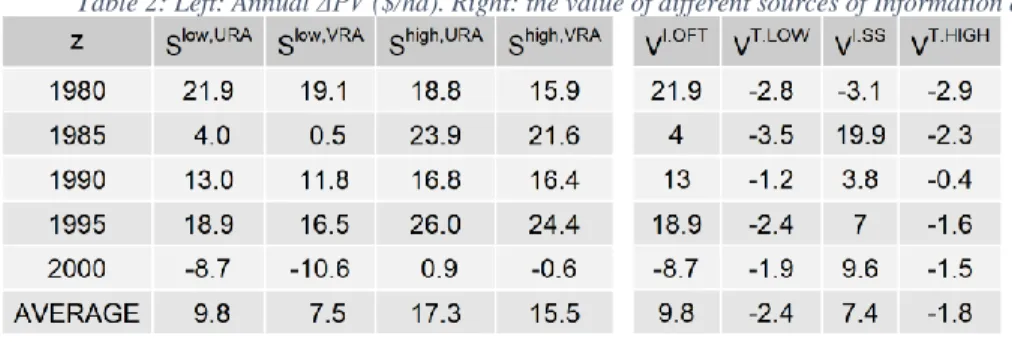
the trials. Key results obtained by this research were: (1) The value of conducting trials and using

that information for N-management advice was 9.8 $/ha. (2) The added value of gathering soil

sampling data at the same time was 7.4 $/ha. (3) The optimal time to stop running trials and start

using the information for N-management advice was one or two years, depending on the

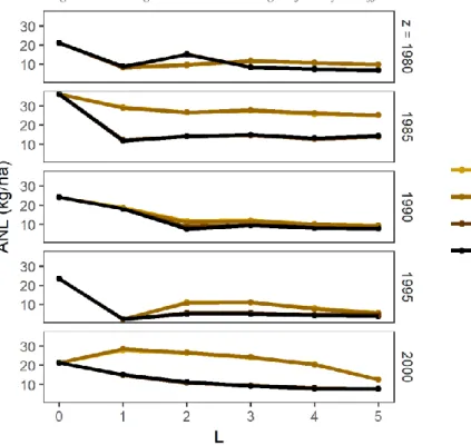
weather. (4) Conducting trials and using that information for N-management advice decreased

leaching by 10.4 kg/ha. Performing soil sampling tests together with running trials made

N-management advice increase the efficiency and reduced N-leaching by 5.9 kg/ha more. (5) A

tentative rule for deciding if a one trial year is sufficient or if one more year is needed was

obtained by determining the likelihood of the weather of the trial year compared with the historic

weather. These results provide insights that will be helpful to optimize the protocol that guide

OFE and help farmers increase profits in the fastest way and decrease the environmental impact

of nitrogen fertilization.

(3)

iii

ACKNOWLEDGEMENTS

I would like to thank Professor David S. Bullock for giving me the opportunity to do my

research in such interesting and current topics, for his energy and passion to conduct the DIFM

project and for all the help he provided during this work.

I am very thankful to Professor Taro Mieno, for his help and availability during all the

working period, for sharing his experience and guiding me step by step in my research.

I am also thankful to Professor Nick Paulson and Professor Nicolas Martin for being part

of my committee and for providing me useful comments in my research.

I am grateful to Fulbright for their fellowship that allowed me to achieve this graduate

study.

I am grateful to Brittani Edge and Rose Keane for reviewing my grammar and answering

all my questions about how to say things and sound professional!

Finalmente quiero decir gracias a mi familia, por estar siempre en cada paso. Por

haberme enseñado a trabajar con el ejemplo y motivarme a dar lo mejor de mí. Por haberme

acompañado en cada pequeña decisión y en cada paso que finalmente terminó conduciéndome a

estar en otro país aprendiendo y desarrollándome.

(4)

iv

1 CHAPTER 1: INTRODUCTION

1.1 EVOLUTION OF ON-FARM, LARGE SCALE FIELD TRIALS

In 1905, the Haber-Bosch process was invented, a process that industrially transforms

nitrogen gas, abundant in the atmosphere, into ammonia, which could be absorbed and used by

plants (Haber, 1905). During the following decades, between the 1930s and the 1960s, a second

shift was produced when crop geneticists began to adapt cultivars to this new way of producing

grains with high inputs (Castleberry et al, 1984). This combination of factors led to increase farm

yields and grew the economic interest in understanding the crop response to inputs. This question

has traditionally been addressed by running field trials that generate data, which is then analyzed

and translated into recommendations for farmers.

Specifically, in corn (Zea Mays L.), this process became very active in the 1950s, 60s and

70s when the numbers of trials and publications increased (Heady and Pesek 1954; Heady et al.

1964, Heady, et al. 1964; Olson et al 1964, Hexem et al. 1976, Shrader et al 1966), opening a

lively debate in major agricultural economics journals about the functional form of crop yield

response functions. This conversation has continued over the last several decades (Swanson et al.

1973; Grimm et al. 1987; Frank et al. 1990; Berck and Helfand 1990; Paris 1992; Bullock and

Bullock 1994; Chambers and Lichtenberg 1996; Llewelyn and Featherstone 1997; MaBL and

Dwyer 1998; Anselin et al. 2006; Tembo et al. 2008; Tumusiime et al. 2011; Brorsen and Richter

2012).

In the first period, the conduction of the trials was done using labor-intensive techniques,

with researchers marking small plots in the field, applying inputs and harvesting by hand or with

small machines, and without the benefit of large-scale farm machinery (Bullock and

Lowenberg-DeBoer 2007). This method was cost intensive, restricting the trials to small plots and mainly on

experiment stations, where workers were available. Recommendations based on these small plots

were extrapolated over large areas (Pan et al., 1997, Bullock, et al. 2002), ignoring variability

and assuming average weather (Swinton and Lowenberg-DeBoer 1998). The results were useful

at this initial stage only to provide a range of Nitrogen (N) rates that could be close to the EONR

with a regional approach for a wide range of field characteristics. This regionals models were not

useful to provide recommendations at a higher detailed level (field or site-specific). For that,

more data, measuring more variables in different sites and weathers was necessary.

(6)

2 With the advent of precision agriculture technology starting in the 1990s, machines were

able to control the applied N rate and measure different variables (like soil electro-conductivity,

applied inputs rates or yield) site-specifically. This technological change shifted the demand for

site specific N management recommendations (Bullock 2013). The previous regional

recommendations were not sufficient to approach this new challenge, and new data needed to be

generated that guided how different site-specific characteristics affected the EONR (Bullock et al

1998).

Fortunately, the same new technology could be used to generate agronomic experiments

at low cost and with a high number of repetitions (Bullock et al 2002, Bullock and

Lowendberg-DeBoer 2007). These advantages provided the groundwork for the following breakthrough in

agronomic experimentation. The new concept is that the same farmers can run on-farm,

large-scale field trials, over many fields to inexpensively gather large amounts of data in multiple field

characteristic and weather (Bullock et al. 2009; Casanoves et al. 2007; Peralta, Cordoba, Costas,

and Balzarini 2013). This new concept of on-farm Experimentation (OFE) is being implemented

by collaborating researchers at the University of Illinois, University of Nebraska, Montana State

University, Washington State University, and Louisiana State University, together with several

international research partners, in an USDA-sponsored project called Data Intensive Farm

Management project (DIFM). This work is originated in that project. The trials implemented by

this working group have a “checkerboard” design and feature a large number of repetitions with

plots small enough to explore similar site characteristics. The trials are also large enough to

collect reliable data from the sensors. Researchers designed the trials for the farmers to conduct

in their field, with minimal change in how they would regularly manage a production crop.

Because experiments are run in an automatized way, it is possible to generate more data at lower

cost than with the previously described labor-intensive plots from the past.

1.2 PURPOSE AND CONTRIBUTION

The project that originates this work has a working protocol, that states the instructions

on how trials are designed, conducted and analyzed. The objective of this work is to explore the

economic value of different strategies that could be used in that protocol, together with the

environmental trade-offs from those field trials, and how that value can be optimized. With

simulations we attempt to address: 1) Is the value of generating on-farm information in trials

(7)

3 likely to cover the cost of conducting such experiments; 2) What is the set of variables that,

measured in the field and incorporated in the model, maximize profits for the farmer?; 3) What is

the optimal number of years to run trials before moving to regular production using the results of

the experimentation as management advice?; 4) What is the environmental benefit of these

different strategies?; and 5) What insights can be used to detect the optimal number of trials in an

ex-ante situation?

Answering these questions will provide insights that can be used to improve the protocol

while helping the associated farmers of the project to make profitable use of the new concept.

The results obtained in this work should not be taken as absolute values, rather as tendencies that

will allow us to move on the path of discovering the best strategy.

1.3 WORK ORGANIZATION

This study is divided into six chapters. Following this introductory chapter, Chapter 2

provides a narrative review of previous studies that also used crop simulation in a spatially

variable field. Chapter 3 is a review focused in providing the conceptual framework for the

methods than will be used later in this study, paying special attention to models that explain and

compare the value of information and technology. Chapter 4 describes the methods used in this

research to create the field, simulate the crop under different situations and strategies, calculate a

model using spatial techniques and finally analyze the results economically. Chapter 5 provides

results from the simulations and discusses these results in detail. Finally, Chapter 6 summarizes

this study’s results and proposes avenues for future research.

(8)

4 CHAPTER 2: PREVIOUS STUDIES USING CROP SIMULATIONS IN

SPATIALLY VARIABLE FIELDS

In Bakhsh et al (2001), the simulation model called Root Zone Water Quality Model

(RZWQM), was used to evaluate the response of soils and crops to different N rates. They had a

data set from 1996 to 1999 of a rotation of corn and soybeans trial data with nine plots where

three different N-rates were applied. Tile flow, NO3-N losses and yield was measured over the

four years. The work showed three parts. In the first part, they calibrated RZWQM by adjusting

some parameters to fit the model output with the real measurements of tile flow data from 1996,

corn yield from 1996 and soybean yield from 1997. Then, in the second part, they evaluated the

model using the data not used during the calibration. The model simulated annual tile flow

adequately, by showing a difference of -8% between measured and simulated values. Similarly,

yield for both crops showed a difference of less than 5% between measured and simulated

values. Finally, in the third part, they use the model to simulate the effect of six different N

rates, including the three tested. The results showed that RZWQM98 model could be used to

assess the effects of N-applications rates on corn yields and NO3-N losses in tile flow, and it may

require further refinements in soybeans. Their article shares with the present work the idea of

using crop simulation to understand the response of corn yield and N losses with different N

rates. Their focus was on calibration and validation of the model, while in the present work no

calibration was performed since we assumed that the model outputs are the real data. Instead, we

focused on creating models that would transform that data into recommendations to farmers,

which can then be evaluated in terms of farmer profits.

Thorp et al (2008) (30) developed a software called APOLLO that allows running

DSSAT, a crop modeling software designed to model a crop in a uniform area, over a spatially

variable area. The most significant incorporation is that it can condense, in a square grid, all the

layers of information that the model needs and then run the model on each of the cells of the

grid. In the second part of the work, they created a spatially variable field and described the

process used to calibrate and validate the model using real data from that same field. Finally, in

the third part they used the system to simulate the effects of climate change over the yield in the

spatially variable field. For this they used two climate scenarios, one from the 1990s and the

(9)

5 other was a future prediction for 2040s. They conclude that climate change will decrease average

yield in this situation and the spatial distribution of higher and lower-yielding areas.

The described software, APOLLO, follows a very similar procedure to the one we use in

this work. We both created a grid condensing spatial information that is needed by the crop

modeling software. The difference is that, instead of using a specially designed software to create

the spatially variable grid and then run the crop modeling software, we performed this procedure

using R (R Core Team 2018). Additionally, their crop modeling software was DSSAT and we

used APSIM (Holzworth et al, 2014). However, the objectives of the two works are different,

since they are predicting the effect of climate change over a field and we are creating trials and

trying to fit models that help to provide advice based on those trials.

Although they described APOLLO in detail in the 2008 work, Thorp et al (2006) used it

to jointly analyze the production function and the environmental externalities of different N rates

in corn. In this work, they created a spatially variable field with 100 cells and, after calibration

with real data, they run 13 N application rates over 37 growing seasons (based on 37 historic

weather years) restarting the field every year to the assumed initial conditions. Their output

included the yield of the crop and the amount of total N unused by the crop. They defined the

profits maximizing rate for each cell as the one that maximized the mean profits of the 37 years.

The environmental rate was determined to be the one that left less than 40 kg/ha of N in soil at

harvest with a probability of 80%. In most of the cases, the profits maximizing rate was higher

than the environmental rate. They calculated the opportunity cost of environmental protection as

the difference in profits of decreasing the rates that were higher to the one that achieve the

environmental goal. That opportunity cost was of $48.12 average for the whole field.

A similar approach to the previous article was followed in Miao et al (2006). In their

work, they divided a field into four management zones based on cluster analysis of multiple soil

layers. After calibrating and validating the model with real data, they used crop modeling with

historical data of the previous 15 years to estimate the EONR, testing different strategies: ex-post

estimation, an average of the EONR for each year and choosing the N rate the maximized the

15-year marginal net return. They mentioned that, although the first approach was the most

profitable, it was not realistic since it is assuming full information. They concluded that choosing

the N rate that maximized the 15-year marginal net return should be the method used by farmers

(10)

6 since it had higher long-term profits than the more straightforward method of averaging the

yearly’s EONR.

The two-last works, Thorp et (2006) and in Miao et al (2006) have much in common with

the present work. The three works used crop modeling to estimate the response of corn to N in a

spatially variable field. One important difference is that they used crop modeling to obtain the

yield response curve and then EONR by running sequential rates for a same site of the field and

calculating the optimal. In our work, each plot of our field had only one N rate each year, not a

sequence. We pretended real trials over the field and crop simulation was used to start thinking

about possible outcomes of those trials.

As presented in the previous review, there has been research using crop modeling

software to simulate spatially variable fields with different objectives. To the best of our

knowledge, no previous economic studies have used it to analyze the problem we will present

here, combining this new concept of running whole field trials and using crop simulation to

obtain the possible outcomes of those trials, compare strategies and finally optimize how those

trials should be run to maximize farmer’s profits.

(11)

7 CHAPTER 3: CONCEPTUAL FRAMEWORK

3.1 NATURE’S META-RESPONSE FUNCTION

To explain how to calculate the value of the new concept of OFE, first it is helpful to

describe the hypothetic function of the response of Yield to inputs. Bullock and Bullock (2000)

and Bullock et. al (2002) provided the “meta-response function” framework to discuss the

concept of how crop yield (Y) responds to all the factors to which is responds. The function

express the Y on a small and uniform site of a field as a function of a vector of “managed inputs”

x = (x1, …, xJ) (decided by the farmer, such us hybrid, seed and fertilizer rates), a vector of

unmanaged spatially dependent “field characteristics” c = (c1 , … , cK) (such as Organic Matter

(OM), elevation, depth of the soil, soil N content) and a vector of stochastic time dependent

variables called “weather” z = (z1,…, zL) (mostly weather variables such as temperature, rain,

radiation, first frost date, but also pest infestations and other factors):

𝑦 = 𝑓(𝒙, 𝒄, 𝒛) (1)

𝑐 = 𝑓(𝒑)

(2)

In this work the concept of past variables p = (p1,…,pm) is incorporated:

This vector is compounded by characteristics of a site measured in the previous season

that affect the present conditions, such as Yt-1, applied Nt-1 rate and the ratio between them Y/Nt-1

(where t-1 means previous year). These past variables do not affect Y directly, if not through an

effect over c. Nevertheless, they may worth being included in the models because with the new

sensors technologies, they have the advantage of being easily measurable at a low cost and being

highly available on most farms. One goal of this work is to explore how using p in the function

would be a promising cost-efficient method to predict the Y response function. For example,

initial N in the soil is a c variable that can be obtained by doing soil sampling (SS), incurring a

certain cost. Instead of using that variable, we can use Y/Nt-1, expecting that when it is high, the

previous crop had used most of the applied N and the residual N in the soil would be low and

vice versa. That way, an important variable of the function, like initial N, can be predicted using

a low-cost variable.

Based on the knowledge of the farmer about the three different vectors, it is possible to

estimate an expected response function. That function can be analyzed and optimized to generate

(12)

8 a field’s application map that maximizes the expected profits for the farmer based on the

available information. When more information is available, the farmer’s decision should be

closer to the true EONR.

3.2 CALCULATING THE VALUE OF TECHNOLOGY AND INFORMATION

In the first stages of precision agriculture, many studies were performed on the

economics of the new technology. Unfortunately, these studies used a wide range of assumptions

and methods (Lowenberg-De Boer 2003). Some of them omitted significant cost, made different

assumptions, or compared profits under different situations. A common mistake had been using

rates obtained without trial data for Uniform Rate Application (URA) versus rates obtained by

analyzing trial data for Variable Rate Applications (VRA), confusing the value of technology

with the value of information (Bullock et al. 2009). A Purdue University review from 2000

showed that the number of economist co-authoring articles was increasing between 1991 and

1999, and several authors outlined methods for obtaining reliable economic estimates of the new

technology (Swinton and Lowenberg-DeBoer 1998, Bullock and Bullock 1998).

Bullock et al. (2009) used a methodology to compare the value of different strategies.

They compared three factors that affect the decisions of the farmer:

• Y response to N knowledge: the knowledge of the exact response function of Y to N rate

(ex-ante, ex-post). “Ex -ante” means that decisions are made before the growing season,

thus the weather is unknown and the farmer does not know the exact yield curve, thus he

must use some historic average. “Ex-post” means that different rates are tested during the

growing season, the exact response curve is known and the optimal N rate selected for

each situation. In “Ex-post” scenario, decisions are optimized for the growing season.

• Information (I): the availability of site-specific information for the field (yes, no). When

more significant spatial variables are incorporate as predictors to a model, the capacity to

explain and predict the response is usually increased. In their work, no information meant

that the farmer had no knowledge of site-specific characteristics and, in that situation, he

had no incentive to use VRA and he would use URA and a regional model to predict the

EONR.

• Technology (T): weather the farmer is using uniform rate application (URA) or has

access to Variable Rate Technology (VRT).

(13)

9 By combining these three factors, eight structures were created combining information

and technology levels.

It can be easily seen how technology can increase profits, by comparing the achieved

profits with and without the technology. It is more complex to see how information affects

profits. According to Lowenberg-DeBoer (1998), information affects profits if it changes

decisions. If certain decisions are more profitable than the ones that would have been made

without the information, the increase in profit is due to the information. Following that

reasoning, a farmer will choose the N rate that maximizes his expected profits on each of the

eight structures. Then, by comparing the change in actual profits, the marginal value of each

structure can be determined.

The economic analysis of this work built over that approach, with slight adaptations. The

first adaptation is that EONR was calculated only in ex-ante conditions. This is because the

interest of the work was analyzing real strategies under partial-information (unknown weather)

and thus, the ex-post EONR is not meaningful for this goal.

The second adaptation is how information is treated. At present, most of the modern

machines used in the U.S. Corn Belt come with sensors to measure different variables. Since the

price of these sensors has been decreasing over time, nowadays most of the base models of

machinery include them. Moreover, that trend is expected to increase in the future. For that

reason, these sensors are assumed a sunk cost, and the information they provide is assumed to be

free. Researchers in the project, in constant contact with farmers, state that it is common to

observe that modern farmers have accumulated over the years many as-applied maps (that is a

map with points where applied rates of the planter or sprayer are recorded), yield maps (that is a

map with points were yield at harvesting is recorded) and elevation maps from their fields over

time, and they are willing to transform it in information that can be useful. For that reason,

instead of having two levels of information (yes or no), three levels were created. One is the “no”

information level and includes the situation where a farmer does not have -or if he/she has does it

is not used for N management purposes- site-specific information and is not running trials. The

“low” information level is the situation where a farmer run trial/s and has free site-specific

information provided by sensors at no cost or insignificant cost. Finally, the third is the “high”

information level and it is the situation where a farmer has information from trials together with

(14)

10 free site-specific information and also gathers soil sampling information every year for initial N

and every four years for OM.

3.3 MAXIMUM RETURN TO N (MRTN)

In 2004, University soil fertility researchers from different States in the corn belt (Illinois,

Iowa, Michigan, Minnesota, Ohio and Wisconsin) with the aim of unifying methods started a

program oriented to provide regional N rate guidelines (Sawyer et al. 2006). In this program,

they collected information from trials across the region, analyzed the data to generate response

models and create, as a final output a N-calculator that is available to the public in their website

(http://cnrc.agron.iastate.edu/).

They way how N-calculator works is allowing the user to select an area within the 6

states, together with management information (rotation, type of fertilizer) and prices of N and

corn. Then the platform provides the result of the model in those conditions, and the suggested

rate to apply to get the Maximum Return to N application (MRTN rate). For the region where the

field is located, the MRTN rate is 224 kg/ha of N.

(15)

11 CHAPTER 4: METHODS

4.1 CONCEPTUAL STEPS OVERVIEW

The present work is compound by two parts. First the data generation process and then

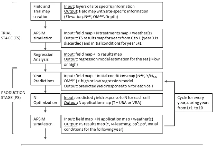
the analysis process. Figure 1 shows the workflow followed during the data generation process.

First, a spatially variable field was created. Over that field, one year of a regular crop using

MRTN rate was simulated to set the initial conditions. That simulation year is not part of the

observations. The research process starts with the Trials Stage (TS), where completely

randomized trials were simulated each year. After TS, the trial information was analyzed, and an

econometric regression model was estimated. The Production Stage (PS) is considered the stage

when the field is used for the regular production of a crop using the EONR obtained from the

trial data.

A ten years-long simulation for the whole field (256 cells x 10 years = 2560

observations), composed by TS and PS is called a set (z,L,S

I,T

). Different sets were created by

combining the following factors:

-

Weather scenarios (z = 1980, 1985, 1990, 1995, 2000): They were created using historic

weather and named based on the first year of the sequence. That means that z = 1980 uses

the weather from 1980 to 1989. Consecutive years of the historic weather were used, to

capture real patterns in the weather.

-

Number of trials (L = 0 to 5): being 0 when no trials were run and L from 1 to 5 the

number of years when a trial was run over the field.

-

Information (I = No, Low, High): No is the situation where no trials were run; Low is

where trials were run and “free” site-specific variables are collected. High is where trials

were run, “free” site specific information is collected and also soil sampling information

of initial Nitrogen (N

Apr

) and Organic Matter (OM

Apr

).

-

Technology (T = URT, VRT) was the technology used during PS, being URT when the

farmer was constrained to select only one rate that maximizes expected profits in the

whole field VRT when the farmer had the ability to select the rate that maximizes

expected profits in each site of the field. It is important to note that during TS the farmer

will always use VRT, because changing the rates that is needed to apply the different

treatments in the trial.

(16)

12 Strategies (S

I,T

_{) was the word used to describe the possible combinations of Technology}

and Information during this work. Since comparisons were done usually by z and at L

OPT

_{, this}

will simplify the notation and avoid repeating the first two superscripts.

In this work, it was assumed that a farmed that did not run trials will not have incentive to

use VRA, and will use only URA of MRTN rate. That way, five S (S

no,URA

, S

low,URA

, S

low,VRA

,

S

high,URA

, S

high,VRA

) were obtained in this work, tested over different L and z.

Having explained what a set and S are, it is possible to account the total number of sets

simulated in this work. The sets are combinations of z,L and S, but not all combinations are

possible. The number of sets that do not involve trials are 5 and they are the combination of

S

no,URA

with L = 0 (if no trials are run, L can only be 0). The number of sets that involves trials

are 100, and they are the combination of the five z (1980,…,2000), with the five L (1,…,5), with

the remaining S that includes trial information (S

low,URA

, S

low,VRA

, S

high,URA

, S

high,VRA

). Adding

them, the total of 105 sets simulated in this work are accounted. Considering that each set is 10

years long and that the whole field has 256 cells, that is a total of 268,800 simulations.

(17)

13

Figure 1: Data generation process workflow

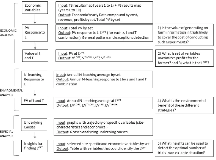
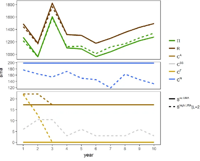
After generating the data, the work continued with the analysis process shown in figure 2.

First, economic variables were computed. The input was the APSIM results map. This map was

condensed into total field values by year (i.e. the N and Y by cell was added for the whole field

to obtain the total N applied and the total grain harvested) and the costs and revenues were

computed by year.

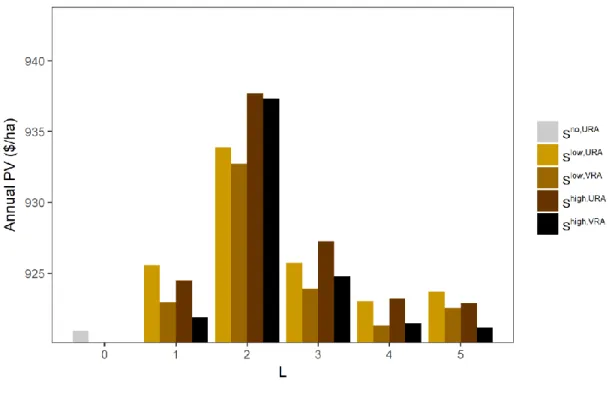
The trajectory of the Present Value (PV) of each set by increasing L was graph and

analyzed to answer question 1 from section 1.2. Using the PV at the L

OPT

, the value of the

different combinations of I and T was obtained, answering question 2 and 3. Then,

Environmental Variables trajectory was analyzed to answer question 4. Finally, two especial

analyses were performed to address question 5, one to understand underlying causes of the

results and the other one to find insights that could help to predict the L

OPT

in ex-ante conditions.

(18)

14

Figure 2: Data analysis process

4.2 FIELD CREATION

4.2.1 INITIAL CONDITIONS

To capture the essence of spatial experimentation and management, a farm field with

spatially heterogeneous field characteristics was modeled. A real 32–ha field owned and

managed by a farmer near Effingham, Illinois (39.1 N latitude and 88.7 W longitude) was used

as starting point.

Spatial site-specific information about elevation, information from soil sampling, and the

soil survey report (SSURGO 2018) were collected. All the variables were edited, following

different procedures. These way, we created a new research field, different than the original, that

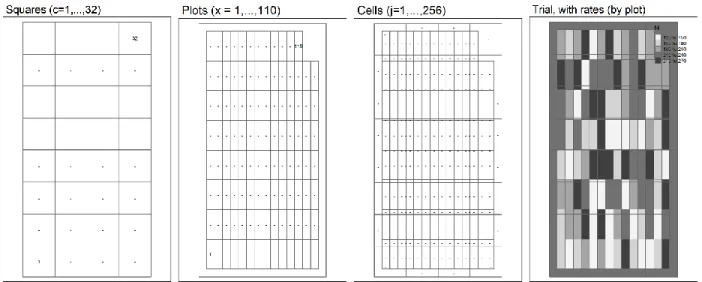
could lead us to explore how variability affects the results. The final product is a square grid

(figure 3) with one-ha cells (c = 1,…,32). Each cell had unique site-specific characteristics

obtained by condensing and editing the different layers of site-characteristics information with

the following procedures:

(19)

15

• Soils: because the soil survey report indicated that 85% of the field is classified under the

same soil type, for simplicity we categorized the whole field under that soil type. This

soil is named Cisne silt loam, with 0 to 2 percent slopes. The typical profile is

Ap-E-Bt1-2Bt2-2C. These soil characteristics were reproduced in APSIM following the

methodology described in Archontoulis et al. (2014).

• Organic Matter in April (OM

Apr

): OM was sampled in April 2016 at 32 points, each at the

center of 1-ha grid cell. Since OM was not highly variable over the field, with a mean of

2.42% and standard deviation of 0.15, the residuals between each measurement and the

mean were multiplied by 1.8 to increase the variation. The final OM

Apr

_{has a mean of}

2.42% and a standard deviation of 0.27. The purpose of this was to explore more

variability in the field that the one present in 2016.

• Nitrogen in April (N

Apr

): is the sum of the quantities N available as N-NO3 and N-NH4 in

April, the day before planting. It was estimated by conducting a linear relation with OM.

Also, a spatially autocorrelated error was added to the result of the function using

Gaussian simulation, according to the following autoregressive process:

𝑁. 𝑖𝑛𝑖𝑡𝑖𝑎𝑙 = 25 ∗ 𝑂𝑀 − 38.52 + 𝑄

(1)

𝑄 = 𝜌

_𝑞

𝑊𝑄 + 𝑒𝑟𝑟𝑜𝑟

𝑒𝑟𝑟𝑜𝑟 ~ 𝑁(0, 𝜎

𝑞2

),

where 𝜌

_𝑞

is the spatial autoregressive parameter, W is the spatial weight matrix,

and 𝜇

_𝑞

and 𝜎

_𝑞2

_{are the expected value and variance of Q. The W is a matrix whose (i,j)}

elements are 𝑒

−0.1∗𝑑𝑖𝑗

_{, where 𝑑}

𝑖,𝑗

is the distance between the centroid of the i-th and j-th

square of the grid.

With this procedure a spatially autocorrelated N

Apr

was obtained for each cell of

the field. N

Apr

values varied among cells between 1 kg/ha and 37 kg/ha.

• Elevation: using high-density point information data from the tractor GPS system, a

point-in-polygon operation was performed, obtaining the median of the elevation points

for each square of the grid.

• Depth: The original thickness of the soil units’ last layers varied between 153 cm and 196

cm. Spatial variation of the total soil depth was generated by varying only the thickness

(20)

16 of the last layer (upper layers were not affected by this procedure). In the same way than

with N

Apr

_{, Depth was calculated as a linear function of Elevation, and an autocorrelated}

errors were added:

𝐷𝑒𝑝𝑡ℎ = 3.183 𝐸𝑙𝑒𝑣 − 1806.46 + 𝑄

(2)

𝑄 = 𝜌

_𝑞

𝑊𝑄 + 𝑒𝑟𝑟𝑜𝑟

With this procedure, a spatially autocorrelated depth was obtained for each cell of

the field, which varied from 153 cm to 200 cm among cells.

As explained before, a set is a 10-year simulation of the whole field. Every set starts with

the field and the initial conditions described above. Then, a regular corn crop was simulated

using a nitrogen fertilizer application at the MRTN rate. These simulations of a regular corn crop

were considered to be in year 0 and they were discarded. Since the initial conditions have an

impact on the result of the trial, the goal of simulating a regular corn before the TS was to expose

those initial conditions to a simulation with a random weather. If this were not done, the first trial

year would always have had the same initial conditions, which would impose the same effect

over the L = 1 strategy in all z scenarios. For example, if the initial conditions have a high N

Apr

_,

then response to N would be low for L=1 and random for higher values of L, which is not

realistic.

4.2.2 TRIAL DESIGN

Over the previously described field, a trial was created following the protocol used in the

DIFM project. A planter machine width of 12 meters was assumed. A border of 24 meters was

created on the edges of the field and considered an area excluded for experimentation. The

reason is that, in real trials, the edges of the field are exposed to uncontrolled factors that

decreased the quality of the data, like winds, heavy machinery transit or different soil quality.

Even though these factors will not be incorporated in the crop modeling simulations, the border

was included because it will change the relative area of the trial and, since the border will receive

the target rate instead of the different treatments, it will have an impact on the economic result of

the strategy.

As shown in figure 3, inside the border, a grid of 110 plots was created. Each plot had 24

m width and 85 m length. When overlapping the initial grid of varying c characteristics, with 32

(21)

17 squares of 1 ha, with the trial design with 110 plots and a border, 256 cells are gotten. Within

these cells, rather the site-characteristics or the received treatment was different. For that reason,

each of these cells was unique and all APSIM simulations were run for each cell. Then, results

were aggregated, to a dimension that represents what we would obtain in a real situation. For

example, if at the time of analyzing the data from the trials, a plot had three cells, all needed

variables were aggregated weighing by area and that that was the data used for the regression

analysis.

With the aim of using the same naming convention throughout the present discussion,

each of the 32 squares in the initial grid was called a “square”. Each of the 110 trial plots that

was created over the field was called a “plot”. Each of the 256 cells with varying dimensions that

have a unique combination of site-characteristics with treatment is called a “cell”.

Figure 3: Naming convention for field layers and resolution

4.2.3 DYNAMIC TREATMENTS

Farmers run annual field trials with a completely randomized design. Each year, five

nitrogen fertilizer rates were randomized on the 110 plots. That is, each one of the five N Rates

were applied on 22 of the 110 plots. The treatments (T) were selected dynamically based on the

following process:

Each year there was a central target rate (TR) and the other 4 rates were calculated based

on this central rate according to: T1= TR – 90 kg/ha, T2 = TR – 60 kg/ha, T3 = TR – 30 kg/ha,

T4 = TR, T5 = TR + 30 kg/ha. Areas along the field perimeter were placed in a “buffer zone,”

not included in the experiment, and assumed fertilized at rate TR. The first trial year, the TR was

(22)

18 the MRTN rate. In subsequent years, the TR was the average among the MRTN rate and the

rates that would have maximized profits in each of the previous trial years.

4.2.4 OTHER MANAGEMENT PRACTICES

All other management practices that are not related with N rate were held constant in all

simulations. Soil sampling was performed on April 29

th

(as explained later, this information

could be used or not, depending on the strategy). The field was tilled every year on April 30

th

of

every year, at a depth of 11 cm, incorporating 40% of the surface residues. The planting date was

May 1

st

of every year. The hybrid was a generic APSIM hybrid with called A110, with 110 days

maturity. The plant population was 8 plants/m

2

and the row spacing was 76 cm. No tiling was

included in the field.

4.3 ON-FARM YIELD CURVE ESTIMATION

4.3.1 SOIL SAMPLING SIMULATION

To make results economically realistic, soil sampling variables needed to be transformed.

High-resolution N

Apr

and OM

Apr

data were provided for each of the 256 cells, by APSIM every

April. Since soil sampling at that resolution would be economically prohibitive, two new

variables were created. They were the spatial and temporal aggregation of the high-resolution

N

Apr

_{and OM}

Apr

_{data. Although this process decreased the precision of the data, it is imitating}

what could be obtained in a real situation.

One of the new variables was the soil N in April obtained by soil sampling (N

Apr.ss

_{). This}

variable was the area-weighted average of N

Apr

_{(whose resolution is by cell) with the following}

soil sampling strategy:

• Year 1: by square. Since the field previously had a uniform-rate crop, variation will

depend on site-specific characteristics that varied by square.

• Year 2 to L +1: by plot. During trial years, since treatments were applied by plot, the soil

sampling was performed at that same scale. Then in the first year after TS (year = L + 1),

since the field still would have high variability in N

Apr

because it had different rates in the

previous year, N

Apr.ss

_{is still performed by plot (and the border area was characterized by}

a single soil sample).

(23)

19

• Year L+2 to 10: by square. Two years after the TS, N

Apr

variation over the field is

smoother, and soil sampling is performed by square.

The other new variable was the soil OM in April obtained by soil sampling (OM

Apr.ss

).

This variable was the area-weighted average of OM

Apr

simulating a soil sampling strategy

performed by square every four years (that is in April of year 1, 5 and 9). That means that for one

of the squares OM

Apr.ss

had the same value from year 1 to 4, then a new value from year 5 to 8,

and finally another new value from year 9 to 10.

4.3.2 MODEL ESTIMATION

In section 3.2 and 4.1, the concept of how Information was treated in this work was

introduced. The level of information of the set will impact the variables included as regressors in

the model estimation. There are three levels of information (no, low, high). If the information

level was no, that means that the farmer did not conduct trials, thus no regression model was

estimated.

If the information level was low, the model included variables that are considered “free”

nowadays. They are the as-applied N, elevation, Y/Nt-1. The N rate is automatically measured by

sensors in the fertilizer applicator that automatically records the rate. The Elevation is recorded

by the guiding system of the tractor. Y is measure by the yield monitor in the harvesting machine

and then transformed to the Y/N ratio. The Low information model was:

𝑌

_𝑖𝑡

= 𝛽

₀

+ 𝛽

_𝑁

∗ 𝑁

_𝑡,𝑖

+ 𝛽

_𝑁2

∗ 𝑁

_𝑡,𝑖2

+ 𝛼

₂

∗ 𝑌𝑒𝑎𝑟2 + 𝛼

₂

∗ 𝑌𝑒𝑎𝑟2 ∗ 𝑁

_𝑡,𝑖

+

𝛼

₂

∗ 𝑌𝑒𝑎𝑟2 ∗ 𝑁

_𝑡,𝑖2

+ 𝛼

₃

∗ 𝑌𝑒𝑎𝑟3 + 𝛼

₃

∗ 𝑌𝑒𝑎𝑟3 ∗ 𝑁

_𝑡,𝑖

+ 𝛼

₃

∗ 𝑌𝑒𝑎𝑟3 ∗ 𝑁

_𝑡,𝑖2

+

𝛼

4

∗ 𝑌𝑒𝑎𝑟4 + 𝛼

4

∗ 𝑌𝑒𝑎𝑟4 ∗ 𝑁

𝑡,𝑖

+ 𝛼

2

∗ 𝑌𝑒𝑎𝑟4 ∗ 𝑁

𝑡,𝑖2

+ 𝛼

5

∗ 𝑌𝑒𝑎𝑟5 + 𝛼

5

∗

𝑌𝑒𝑎𝑟5 ∗ 𝑁

_𝑡,𝑖

+ 𝛼

₅

∗ 𝑌𝑒𝑎𝑟5 ∗ 𝑁

_𝑡,𝑖2

+

𝛽

𝐸

∗ 𝐸

𝑖

+ 𝛽

𝐸𝑁

∗ 𝐸

𝑖

∗ 𝑁

𝑡,𝑖

+ 𝛽

𝐸𝑁2

∗ 𝐸

𝑖

∗ 𝑁

𝑡,𝑖2

+ 𝛽

𝑌/𝑁

∗ 𝑌/𝑁

𝑡−1,𝑖

+ 𝛽

𝑌.𝑁 ∗ 𝑁

∗ 𝑌/𝑁

𝑡−1,𝑖

∗ 𝑁

𝑡,𝑖

+ 𝛽

𝑌/𝑁∗𝑁2

∗ 𝑌/𝑁

𝑡−1,𝑖

∗ 𝑁

𝑖2

+ ε

𝑡,𝑖

(3)

𝑤ith ε

_𝑡,𝑖

= λWε

_𝑡,𝑖

+ 𝑢

_𝑡,𝑖

𝑎𝑛𝑑 𝑢~𝑁(0, 𝜎

2

_𝐼𝑛)

Where,

(24)

20 𝛽

₀

is the parameter for the intercept,

𝑌𝑒𝑎𝑟2 𝑡𝑜 𝑌𝑒𝑎𝑟5 are dummies variables for the respective year. When combine with the

respective parameter 𝛼

₂

𝑡𝑜 𝛼

₅

they constituted the year effect, representing the change in the

quadratic response relative to year 1 (omitted category). They estimated unobserved

characteristics that are specific to a particular year,

𝑁

_𝑡,𝑖

is the N rate, 𝐸

_𝑖

is the Elevation, 𝑌/𝑁

_{𝑡−1,𝑖}

is the Y/N ratio from the previous year,

If the information level was high, the model included all the low information variables,

but also incorporated the soil sampling information. The High information model was:

𝑌

_𝑖𝑡

= 𝛽

₀

+ 𝛽

_𝑁

∗ 𝑁

_𝑡,𝑖𝑇

+ 𝛽

_𝑁2

∗ 𝑁

_𝑡,𝑖𝑇 2

+ 𝛼

₂

∗ 𝑌𝑒𝑎𝑟2 + 𝛼

₂

∗ 𝑌𝑒𝑎𝑟2 ∗ 𝑁

_𝑡,𝑖𝑇

+

𝛼

2

∗ 𝑌𝑒𝑎𝑟2 ∗ 𝑁

𝑡,𝑖𝑇 2

+ 𝛼

3

∗ 𝑌𝑒𝑎𝑟3 + 𝛼

3

∗ 𝑌𝑒𝑎𝑟3 ∗ 𝑁

𝑡,𝑖𝑇

+ 𝛼

3

∗ 𝑌𝑒𝑎𝑟3 ∗ 𝑁

𝑡,𝑖𝑇 2

+

𝛼

₄

∗ 𝑌𝑒𝑎𝑟4 + 𝛼

₄

∗ 𝑌𝑒𝑎𝑟4 ∗ 𝑁

_𝑡,𝑖𝑇

+ 𝛼

₂

∗ 𝑌𝑒𝑎𝑟4 ∗ 𝑁

_𝑡,𝑖𝑇 2

+ 𝛼

₅

∗ 𝑌𝑒𝑎𝑟5 + 𝛼

₅

∗

𝑌𝑒𝑎𝑟5 ∗ 𝑁

_𝑡,𝑖𝑇

+ 𝛼

5

∗ 𝑌𝑒𝑎𝑟5 ∗ 𝑁

𝑡,𝑖𝑇 2

+

𝛽

_𝐸

∗ 𝐸

_𝑖

+ 𝛽

_𝐸𝑁

∗ 𝐸

_𝑖

∗ 𝑁

_𝑡,𝑖𝑇

+ 𝛽

_𝐸𝑁2

∗ 𝐸

_𝑖

∗ 𝑁

_𝑡,𝑖𝑇 2

+ 𝛽

_𝑌/𝑁

∗ 𝑌. 𝑁

_{𝑡−1,𝑖}

+

𝛽

_{𝑌/𝑁 ∗ 𝑁}

∗ 𝑌/𝑁

_{𝑡−1,𝑖}

∗ 𝑁

_𝑡,𝑖𝑇

+ 𝛽

_{𝑌/𝑁∗𝑁}2

∗ 𝑌/𝑁

_{𝑡−1,𝑖}

∗ 𝑁

_𝑡,𝑖𝑇

+ 𝛽

_𝑂𝑀

∗ 𝑂𝑀

_𝑡,𝑖𝐴𝑝𝑟.𝑠𝑠

+

𝛽

_𝑂𝑀𝑁

∗ 𝑂𝑀

∗ 𝑁

_𝑡,𝑖𝑇

+ 𝛽

_𝑂𝑀𝑁2

∗ 𝑂𝑀

∗ 𝑁

_𝑡,𝑖𝑇 2

+ ε

_𝑡,𝑖

(4)

𝑤ith ε

𝑡,𝑖

= λWε

𝑡,𝑖

+ 𝑢

𝑡,𝑖

𝑎𝑛𝑑 𝑢~𝑁(0, 𝜎

2

𝐼𝑛)

Where,

𝑁

_𝑡,𝑖𝑇

(Total Nitrogen), is the sum of 𝑁

and 𝑁

𝑡,𝑖

rate,

𝑂𝑀

is the OM obtained by soil sampling.

In statistics, Ordinary Least Squares (OLS) is an estimation method for the unknown

parameters that assumes that errors in the dependent variable are uncorrelated with the

independent variable(s). When this is not the case, OLS would not provide unbiased model

estimates. For that reason, in this work, statistic procedures that allow spatial autocorrelation,

were used to estimate the unknown parameters.

(25)

21 In spatial statistics there are different options for including spatial autocorrelation in a

model. Given the characteristics of the variables in this work (𝑁

_𝑡,𝑖

, 𝐸

_𝑖

, 𝑂𝑀

, 𝑁

_𝑡,𝑖𝑇

, 𝑌/𝑁

_{𝑡−1,𝑖}

),

no spillover could exist between the different plots. The treatments were applied only in the

target area, affecting the Yield of that site and not the neighbors. Moreover, a change in the

regressors would not affect the Yield of a neighbor indirectly (no spillover effect). For that

reason, the only model for spatial autocorrelation that could be used is the Spatial Error Model

(SER). When only one year of data was available (L=1), the “errorsalm” function from the R

package “spdep” (Bivand et al. 2013, Bivand and Piras 2015) was used. If more than one year of

data was available (L > 1) the Spatial Panel Error model from the R package “splm” was used

(Giovanni and Piras 2012).

4.3.3 SOURCES OF ERROR FOR THE MODEL

In this work, data was simulated using APSIM based on all the provided inputs. Then, a

regression model was adjusted over that data using less information, or with different spatial and

temporal resolution. In consequence, the regression did not explain all the variability, having a

random error - ε

𝑡,𝑖

in (1) and (2). In this section, the sources of that random error are explained in

detail:

-

Omitted variables: Depth was one of the inputs in the APSIM simulations and it affects

Yield, especially in dry years, since it changes the amount of water that the soil can retain.

This variable was not included in the regressions directly, it was included indirectly since it is

correlated with Elevation. The two other omitted variables were N

Apr.ss

_{and OM}

Apr.ss

_{in the}

low information model. The portion of the variability explained by the omitted variables

would be part of the error in the model.

-

Soil sampling representation: since soil sampling is costly, in the high information model,

N

Apr

and OM were spatially and temporally aggregated based on the procedure explained in

4.3.1. This decreased precision of the data, increasing the error of the model.

-

Spatial resolution: The field had 256 cells and APSIM is run every time for each cell. One

plot can be composed by more than one cell. For the regression model estimation, variables

were aggregated doing and area-weighted averaged to obtain one observation per plot (total

of 110 observations). All the variables in the model were affected by this process 𝑌

_𝑖𝑡

, 𝑁

_𝑖𝑡

, 𝐸

_𝑖

,

𝑂𝑀

, 𝑁

_𝑡,𝑖𝑇

, 𝑌/𝑁

𝑡−1,𝑖

).

(26)

22 In the case of 𝑁

_𝑡,𝑖𝑇

and 𝑂𝑀

they were aggregated twice, first according to the

soil sampling resolution and then, if a plot had more than one value, it was again

aggregated by plot.

-

Functional form: APSIM is not an equation, it is a crop modeling software with modules that

interact which each other. In this work, a quadratic functional form was used and it has not

necessarily the exact same shape than the APSIM output, increasing the error term.

-

Weather not captured by year fixed effect: To make the model applicable in a wider range of

situations, the year effect was incorporated only affecting the quadratic response of Y to N

and the intercept, not the other regressors. If it also interacted with other variables, the

interaction will be part of the error term.

4.4 EONR PREDICTION

4.4.1 WEATHER WEIGHTED PROFIT FUNCTION

During PS, every April, yield predictions for each cell for each year were obtained using

the corresponding regression model, the initial conditions of the cell in April for that year and an

increasing sequence of N rates. As a precaution, the included sequence ranged from the lowest

tested rate in the trial to the highest, to avoid extrapolations outside the tested rates.

Some considerations were made regarding the year dummy variables. The model for L >

1 had a fixed year effect variable interacting with the intercept, the linear and the quadratic

response to N (or N

T

) in the high information model. These year fixed effects are for past years

and, at this time of the process, we need to predict the EONR for the future year, in ex-ante

conditions, with uncertainty in the weather. To do this, the yield for each N in the sequence rates

was calculated using each year fixed effect. Then, Partial Profits were calculated considering the

price of corn (P

C

= 0.157 $/kg = 4 $/bu) and the cost of Nitrogen (P

N

= 0.881 $/kg = 0.4 $/lb). All

other costs are assumed to be the same for all rates and not considered at this part of the work

since they will not affect the optimization process. For example: if L = 3, a dummy variable for

year 2 and year 3 was added to the sequence of N rates, and three response curves of profits to N

were created for each cell.

The profit curves for each year were condensed in one weather weighted profit

function. For this, a probability of occurrence was assigned to each of them. This probability

(27)

23 was calculated using the historic weather and assuming a normal distribution of it. Two weather

variables were used: Season precipitation (pp

S

_{) and July precipitation (pp}

J

_):

-

𝑝𝑝

_𝑡𝑆

: is the amount of precipitation from sowing to harvesting during year t. pp

S

_affects

two processes. On one hand, if the crop is limited by water, an increase in pp

S

would

produce a higher response of the yield to N, because it will increase the growing rate of

the plants and with that the uptake of N. On the other hand, an increase in pp

S

is

associated with an increase of leaching, especially if the precipitations are concentrated

in the stages were the growing rates (and thus the N uptake) are low.

-

𝑝𝑝

_𝑡𝐽

: is the amount of precipitation in July of year t. July is the month of the year where a

crop planted at the beginning of May will be flowering. The -15 and +15 days before and

after flowering are the Critical Period of the crop, when the crop generates the potential

grains and thus the availability of resources produce a great impact on yield. As a result,

high values of pp

J

are associated with a higher capacity of the crop to uptake N and

generate in Y. In contrast, water limitations in this period will reduce the Y of the crop

and the demand of N.

Is important to consider both variables, because they could have different effects on the

crop-soil system. For example, it is expected that a high pp

S

in combination with a low pp

J

will

produce a high N-leaching without increase in Y. This is because the precipitations will be

concentrated in a period of the season when the crop is not growing fast and up-taking N, thus

the N in the soil will be transported below the roots depth. If a normal pp

S

is combined with a

high pp

J

it is expected to have a high response of Y to N, and not much over the N-leaching,

since the crop is receiving water in the moment when it is at full capacity to uptake the nutrient

from the soil and generate grains.

For that reason, both variables were combined to determine the probability of each year,

doing the following procedure:

With Season precipitation

𝑍

𝑡𝑆

=

𝑝𝑝𝑡𝑆− 𝜇 𝑝𝑝𝑡𝑆 𝜎 𝑝𝑝𝑡𝑆

(5)

With July precipitation

𝑍

_𝑡𝐽

=

𝑝𝑝_𝑡𝐽− 𝜇 𝑝𝑝𝑡𝐽 𝜎 𝑝𝑝𝑡𝑆

(7)

(28)

24 𝑃𝑍

_𝑡𝑆

= 𝑃(−𝑎𝑏𝑠(𝑍

_𝑡𝑆

)) (6)

𝑃𝑍

_𝑡𝐽

= 𝑃 (−𝑎𝑏𝑠(𝑍

_𝑡𝐽

)) (8)

Combined probability of both weather variables:

𝑊𝑃

_𝑡

=

𝑃𝑍𝑡𝑆 𝑃𝑍𝑡

𝐽

∑𝑡=𝐿_𝑡=1(𝑃𝑍_𝑡𝑆 𝑃𝑍_𝑡𝐽)

(9)

Where 𝜇 is the mean and 𝜎is the standard deviation of the indicated variable. Then, 𝑍 is

the distance between each of the observed values and the respective historic mean in units of

standard deviation.

𝑃(−𝑎𝑏𝑠(𝑍)) is the accumulated probability of the negative of the absolute value of the Z

score (left side of the distribution), assuming that Z ~ N(0, 1)

With this method, the Weather Probability (WP

t

) of each profit function was calculated

considering how usual was the combined weather of both variables. This allowed to decrease the

weight of trials run in years with a weather that is not expected to happen in the future, and

increase the weight of those whose weather is more likely to happen.

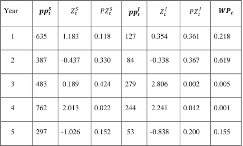
To explain this, the example in table 1 is provided. With z = 1990, 5 trials were

conducted (L = 5). The historic weather from 1979 to 2015 has a 𝜇

_𝑃𝑝

𝑡𝑆

= 454 , 𝜎

𝑃𝑝𝑡𝑆

= 153,

𝜇

_𝑃𝑝

𝑡

𝐽

= 105 and 𝜎

𝑃𝑝_𝑡𝐽

= 62. In this example, year 4 was an extremely wet year, both for the total

amount during the Season and during July. If we calculate the profits as a regular average of the

5 productions functions, we would assign year 4 a probability of 20%. With this methodology we

will assign it a probability of 0.1%. Year 3 had a

𝑃𝑝

_𝑡𝑆

_{very close to the mean and thus, highly probable. Nevertheless, 𝑃𝑝}

𝑡

𝐽

was extremely high,

with a very low probability. This last characteristic decreased the final probability of year 3 to

0.5%. The weather weighted profits function will be mainly a combination of year 2 (61.9%),

year 1 (21.8%) and year 5 (15.5%).

(29)

25

Table 1: Year fixed effects aggregation example, using the weather scenario starting in year 1990.

Year 𝒑𝒑𝒕𝑺 _𝑍𝑡𝑆 _𝑃𝑍𝑡𝑆 𝒑𝒑𝒕 𝑱 𝑍𝑡 𝐽 𝑃𝑍𝑡 𝐽 _𝑾𝑷 𝒕 1 635 1.183 0.118 127 0.354 0.361 0.218 2 387 -0.437 0.330 84 -0.338 0.367 0.619 3 483 0.189 0.424 279 2.806 0.002 0.005 4 762 2.013 0.022 244 2.241 0.012 0.001 5 297 -1.026 0.152 53 -0.838 0.200 0.155

4.4.2 RESOLUTION AND TECHNOLOGY

In section 4.2 and Figure 3, the naming convention of square, plot and cell was stated.

The model was generated using as data the trial information, where each of the 110 plots was an

observation. The reason why data was aggregated to one observation per plot is that, under a real

situation, it takes time and distance to the spraying machine to change from a rate to another,

especially when rates are separated one from another like in a trial. Also, the yield monitor has a

lag between it finishes processing one plot and the harvesting machine has enough flow of grain

from the following plot, to provide a quality measure of grain.

During PS, the change in rates over the field is expected to be smoother than over the trial

and it was assumed that the sprayer could apply the target rate and that the yield monitor was

able to provide quality measures of yield for each of the 256 cells. For that reason, even though

the model was generated at the plot level -i.e. using plots as observations-, the predictions were

done at the cell level.

After calculating the weather weighted profits function for each of the squares there are

two possible paths to proceed:

If the farmer was going to use URA during PS, he had the restriction of using only one

rate in the whole field. For that, all the weather weighted profits function for each cell were

combined in only one for the whole field. This was done by adding the gross profits of each cell

(considering the area) for each N rate. Then, the N rate that maximized the profits for the whole

field was selected (𝐸𝑂𝑁𝑅

_{𝑈𝑅,𝑡}

). This is the rate that will be applied the following year uniformly

over the field.

(30)

26 On the other hand, if the farmer is using VRA during PS, the weather weighted profits of

each cell for each N rate was calculated. Then, the N rate that maximized profits was selected

(𝐸𝑂𝑁𝑅

_{𝑉𝑅,𝑡,𝑗}

). This was the rate that will be applied the next year on each cell, using VRA.

4.4.3 SOURCES OF ERROR FOR THE PREDICTIONS

The predictions of yield and profits for a future year were made using the model that has

a random error term ε

_𝑡,𝑖

whose composition was explained in 4.3.3. Since the predictions are

made for future conditions, instead of past, new sources of error are added:

• Different weather: predictions are obtained for a future year, with unknown weather. The

weather weighted profit function created with the historic weather could be different than

the one that will be experienced during the next growing season.

• Extrapolation in initial conditions: the initial conditions in April can have a different

combination of values in the different variables of the model than the ones explored

during the trial years. Thus, the predictions would extrapolate values outside the

evaluated range that could lead to error in the predictions. For example, the model could

be created with a range of variation in Y/Nt-1 and applied afterwards in a different range.

• Spatial aggregation of N

Apr

: After TS, N

Apr

is aggregated. The first year, the aggregation

is at a plot level and then at a 1 ha square grid level. This reduce the precision of the

model.

• Evaluated rates: each trial had five treatments rates, with rates separated by 30 kg/ha.

Prediction of the Y response to N were calculated using a N sequence that goes from the

maximum N rate used in the trial to the minimum N rate use in the trial, by 10 kg/ha . In

consequence, there is interpolation between the rates used for generating the model and

the rates used for the predictions.

4.5 ECONOMIC ANALYSIS

For each set(z, L, S

I,T

), all the cost related with N management was tracked and

considered in the economic analysis. During TS, the cost of the farmer’s extra effort and time

that takes to learn and implement the experiment on year t was called 𝐶

_𝑡𝐹

. In the DIFM project,

new farmers that are starting to participate in the project for the first time, are invited to a

two-hour meeting where they are informed about the basic experimental procedures. Including the

(31)

27 travel and the time, an opportunity cost of $200 was determined for attending this meeting. Also,

researchers of the project have noticed that there is a learning curve of farmers, where the first

year they have frequent questions related with the conduction of the experiments, and in

subsequent years consultation becomes less necessary. For that reason, a lump sum of $500 was

considered the first year as a compensation for the communication effort and time of the farmer.

This sum was decreased to $400 for year two, $200 for year 3 and $100 for the remaining years

of experiments. Adding both items, 𝐶

₁𝐹

=$700, 𝐶

₂𝐹

=$400, 𝐶

₃𝐹

=$200 and 𝐶

_𝑡>3𝐹

=$100 for the

remaining years

𝐶

_𝑡𝐴

was the total cost of applying N on the whole field during year t. The price charged by

fertilizer applications service providers vary in the U.S. Corn Belt. Plastina, Johanns, and Erwin

(2016) reported an average charge of 16.43 $/ha for URA of liquid fertilizer from a survey in

Iowa. For those same services, Miller (2013) reported an average charge of 15.17 $/ha from a

survey of Indiana, Stein (2014) reported an average charge of 18.78 $/ha by custom applicators

in Michigan, and Halich (2016) reported an average 14.82 $/ha in Kentucky. Halich (2016) also

stated that custom applicators in Kentucky charged 4.94 $/ha more for VRA (instead of URA)

dry fertilizer. In this work it was assumed that the price that service providers charged is

P

VR

=22.39 $/ha for VRA and P

UR

=$17.3 $/ha for URA. During TS, 𝐶

𝑡𝐴

is obtained by doing the

area of the field times the P

VR

, because VRA is needed to run the trial. During PS, when VRA

was used, 𝐶

𝑡𝐴

is also calculated doing the area of the field times P

VR

. In contrast, when URA was

used, 𝐶

_𝑡𝐴

is the area of the field times P

UR

_.

𝐶

_𝑡𝐶𝐶

denotes the cost of soil sampling to obtain N

Apr.ss

and OM

Apr.ss

. The cost of soil

analysis in a laboratory in the Midwest was assumed to be $4/sample for N and $4/sample for

OM

Apr.ss

Using crop simulation to optimize variable rate experimentation