Yield Book Advanced Topics

(1)

Yield Book Advanced Topics

(2)

Yield Book Advanced Topics

Version 1-17-02

These materials and the information and methodologies described and incorporated herein are proprietary and confidential to The Yield Book Inc. and may not be disclosed to third parties, or duplicated, or used for any purpose not expressly authorized by The Yield Book Inc. Any unauthorized use, duplication, or disclosure of these materials, information, or methodologies is prohibited by law and will result in prosecution. The Yield Book Inc Inc.

388 Greenwich Street New York, NY 10013 (212)816-BOOK

The Yield Book® is a registered service mark of The Yield Book Inc Throughout this documentation, “Yield Book” refers to The Yield Book® analytical software.

(3)

i

Single Currency Return Attribution: Methodology ... 1-1

Overview of Methodology ... 1-3 Return Attribution: Page Layout by Steps ... 1-7 Individual Security Return Attribution: Example ... 1-11 Methodology Example: Scenario Analysis... 1-17 Calculation of Components... 1-21 Current Coupon Spread... 1-25 Introducing Dynamic Portfolios ... 1-30 The IRR Method for Averaging Returns... 1-31 Examples... 1-32 Allocation of Returns to Sector and Issue Level Components 1-35 Examples: Sector and Issue Allocation... 1-39 Example #2: Treasury and Agency Broken Down... 1-44 Comparison of Sector Weight and Issue Selection ... 1-45

Return Attribution: Examples ... 2-1

Return Attribution Implementation: Examples... 2-3 Example #1: Static Portfolio using SSB Pricing ... 2-3 Example #2: Static Portfolio vs. Index ... 2-9 Example #3: Duration Override... 2-25 Example #4: Prepayment Override View... 2-27 Custom Data View ... 2-29 Reporting... 2-29 Custom Setup ... 2-31 Example #5: Custom Setup... 2-33 Active Portfolios with Transactions... 2-34 Entering Transactions ... 2-37 Returns and Attribution on Dynamic Portfolio... 2-41 Entering Transactions using a YbPort Update File... 2-45 Trading Prior to Dated Date in Return Attribution ... 2-46 General Notes about Return Attribution ... 2-47

Multi-Currency Return Attribution: Methodology ... 3-1

Return Attribution on Non-dollar Securities... 3-2 Methodology and New Terms... 3-3 Equations... 3-4 Example: Multi-Currency Portfolio vs. Index ... 3-7 Hedge Strategy Notes: ... 3-13 Bond Examples ... 3-15

(4)

Contents

ii

Allocation of Return in Multi-Currency Portfolios ... 3-21

Optimization ... 4-1

Optimization Terminology... 4-3 General Optimization Procedure... 4-5 Objectives and Constraints... 4-7 Get Started ... 4-9 Constraint Definitions ... 4-10 Constraint Functions ... 4-11 Defining the Constraint “Side” ... 4-15 Per-issue Constraints... 4-17 Constraints Relative to Baseline Portfolios ... 4-18 Removing Constraints from Optimization... 4-21 Constraint Files ... 4-21 Soft Constraints and Penalty Function... 4-22 Examples Using Optimization in Buy/Sell Mode... 4-25 Example 1: Effective dv01 Neutral Trade... 4-27 Example 2: Hedging Corporates with Treasuries ... 4-33 Optimization in Own/Universe/Baseline Mode ... 4-39 Example 3: Constructing a “Tracking” Portfolio... 4-41 Formulating the Problem ... 4-45 Example 4: Optimize Portfolio Relative to a Benchmark... 4-49 Example 5: Track a Benchmark using Soft Constraints ... 4-57 Reports for Optimization Results... 4-65

Optimization: Examples ... 5-1

Example #1: Trade Weighting ... 5-3 Example #2: Mortgage Index Tracking Portfolio ... 5-19 Example #3: Corporate Index Tracking Example... 5-29 Example #4: Cash Matching... 5-41

(5)

WORKSHOP

Salomon Analytics Inc.

Single Currency Return Attribution:

Methodology

Agenda

The Salomon Smith Barney (SSB) Return Attribution Model in the Yield Book calculates and dis-sects total returns of single or multi-currency fixed income securities, trades, portfolios and/or indices into return attribution factors. The attribution factors explain why the bond achieved the return that it did.

The model is designed to calculate and explain returns by decomposing the total return of each secu-rity into several attribution components. The attribution components correspond to the effect of the passage of time and various market changes such as yield curve movement, changes in volatility, mortgage prepayment rates, and changes in spreads. The analysis is implemented using SSB’s ana-lytic models including: Yield Curves, Term Structure Model, and Mortgage Prepayment Models to measure the effect of these market changes on each security.

The model analyzes portfolios and indices by aggregating the issue level return components to the sector level. The sector level aggregation allows the model to measure the effects of portfolio strate-gies such as sector weighting and issue selection.

Highlights

In this section of the advanced workshop chapter, we will cover the following:

• The Layout of the Return Attribution Page

• Understanding the Return Attribution Model Methodology and the Components of

Return on Individual Securities

• Calculating the Average Return and Portfolio Attribution Components on Static

ver-sus Dynamic Portfolios

(6)

1-2 Single Currency Return Attribution: Methodology

Return Attribution Components: Detail

Total ROR

Spread

Advantage

Benchmark

Rolling Yield Market Parallel Shift Reshape Spread Market Current Index/ Convexity Advantage

1

2 ₃

4

5 ₆

7

8

9

10

Volatility

11

12

Prepay

Difference Coupon Spread

On-the-Run Spread Spread Change Change Swap Reshape Advantage Change Change Spread Change

(7)

Overview of Methodology

Single Currency Return Attribution: Methodology 1-3

Overview of Methodology

Return Attribution is calculated in three major steps:

Step 1: Calculate Issue Level Attribution Components

Step 2: Calculate Portfolio Level Attribution Components from the Individual Securities

Step 3: Allocate either the Total Return or just the Spread Advan-tage (non-treasury portion) Return into Sector and Issue Effects.

In this section we will cover the first two steps. The third step will be cov-ered in section 3 of this handbook.

Step 1: Calculate Issue Level Attribution Components

The major dissection of every security’s return is to measure what is due to the yield curve exposure or the “treasury” portion and what is due to everything else. The everything else term, is referred to as “spread

advantage”. This first level break down is shown in the top of the

dia-gram on the opposite page. In order to calculate the treasury component, we must first construct what we call the “Matched Benchmark

Portfo-lio (MBP)” for the bond. The construction of the “MBP” will be

explained later.

The attribution analysis consists of up to 12 scenario analyses for each security or it’s MBP. In each scenario, the settlement date is the begin-ning of the attribution analysis period and the horizon date is set to the end of the attribution analysis period. In each successive scenario analy-sis, one input is changed and one additional return attribution component is captured. The 12 attribution components are numbered in the diagram on the opposite page. The successive scenario analysis method decom-poses the security’s total ROR into components corresponding to the effects of various systematic market changes. The remaining return is attributed to spread change.

Analytic Assumptions: The Return Attribution methodology requires that you use the following pricing assumptions:

Curve Volatility Settle

Tsy/Agn/Corp Tsy Model 10% Same Day (begin or end of

analy-sis period)

Mortgage Tsy Model Market Same Day (begin or end of

(8)

Return Attribution Components: Issue/Sector

Total ROR

Spread

Advantage

Treasury

Sector

Weighting

Issue

Selection

(9)

Overview of Methodology

The Return Attribution Matrix

The twelve issue level attribution components can be categorized and summarized in a two-dimensional matrix as shown on the top of the opposite page.

Dimension by Row: Benchmark vs. Spread

The first dimension in the table is displayed in the rows: the breakdown between Benchmark-like Return Components (as calculated through the MBP) and the Spread-like Components.

Dimension by Column: Yield Effect vs. Market Effects

The second dimension in the table is displayed in the columns: the breakdown between the Yield Effect and the Market Effects.

The row and the column totals also provide important measures such as

Spread Advantage (i.e. the total incremental return of the security over

the MBP).

Step 2: Calculate

Portfolio Level Attribution from the Individual Security Data

Once the calculation of issue level attribution components are completed, you can combine securities to look at portfolio level components. The method to average these securities depends on whether the portfolio was static or active over the return period. We will explain both averaging methods in detail.

Step 3: Allocate Spread Advantage Return into Sector and Issue Affects.

Performing the return attribution analysis on an entire portfolio and its corresponding Index allows us to further allocate the portfolio’s Spread

Advantage return component into Sector Weighting and Issue Selec-tion components as shown in the diagram on the bottom of the opposite

page. A detailed example will be covered later, but the basic equations used to calculate these components are:

Sector Weighting in Sector =

(Index spread advantage in sector - Total Index spread advantage) * (Portfolio Overweight in sector)

Issue Selection in Sector =

(Portfolio spread advantage in sector - Index spread advantage in sector) * (Portfolio Weight in Sector)

• Note: The basic allocation of return into sector and issue level components is done on the Spread Advantage Return, which is the return after the treasury effects (dura-tion and yield curve reshaping) are broken out. Some users may wish to allocate the Total Return into Sector and Issue level components including the treasury portion. This is also available and will be explained and shown in a later example.

Before going through a specific example to understand the methodology, let’s first see the layout and general procedures of the Return Attribution page (Chapter 4, Page 6) in the Yield Book.

(10)

Return Attribution: Page Layout by Steps

1

(11)

Return Attribution: Page Layout by Steps

Return Attribution: Page Layout by Steps

Please be aware that the steps in the Return Attribution page for calculat-ing return attribution are the same for either a static or an active portfolio. The additional step needed to analyze active portfolios is to define and save transactions to the portfolio. This is done in other pages of the Yield Book, and can be done daily or at the end of a period. Once you are ready to run the attribution on either a static or active portfolio, the following steps are taken in the attribution page, Chapter 4.6. Let’s review the steps as circled in the picture on the left:

Step 1: Issue Select Retrieve issues, portfolios, or indexes on the buy and/or sell side. You can either retrieve the issues that are sitting in Ch. 4.2 [Receive Buy or Sell from 4.2] or you can retrieve a saved portfolio [Portfolio].

Note about Portfolios with Transactions: The portfolio composition is defined at the beginning of the analysis period and all of the transactions (buys, sells, cash inflows, cash outflows) over the period are saved with the portfolio.

Step 2: Pricing Define the begin and end pricing parameters for the calculations. This includes yield curves, settlement dates, and prices of bonds. The easiest way to define these is to use price files [Price File]. If you do not have saved price files of your own and you do not want to use SSB global price files, you have the ability to price the bonds manually through the [Pric-ing Page].

Step 3: Calculations Run returns only by toggling <ROR> or run returns with return attribu-tion calculaattribu-tions by toggling <RET ATT>.

[Read Results] is there to retrieve pre-calculated results. We provide you with pre-calculated results on a daily and monthly basis for the universe of Salomon Index bonds.

[Custom Setup] is available for those who wish to customize the partial duration calculation used to calculate the “MBP” and/or limit the number of attribution factors that are calculated.

Step 4: Output The [Print or Copy Summary] generates a canned return attribution sum-mary report of the buys and/or sells. The [Report] button takes you to the template and sector selection page in Ch. 4.2 so you can generate issue level or sector level reports. You may also [Save Results] after calculating for retrieval in the future.

(12)

Return Attribution: Page Layout

7 ₈

5

6

(13)

Return Attribution: Page Layout by Steps

Return Attribution: Page Layout

The remaining sections of the Return Attribution page provide informa-tion on the inputs and outputs of the return attribuinforma-tion calculainforma-tion. Each section is circled on the opposite page.

Navigation: #5 These navigation buttons are similar to other areas of the Yield Book. You can scroll up and down through the issues, compress issues in or out, sort issues, and focus in on a certain subset of bonds.

Data Views: #6 The data view defines what values are displayed for the issues in the list-box. There are six global views and one Custom view where you can cus-tomize a template and read in into this page. The global views will be shown in detail later.

Yield Curve: #7 The Yield Curves displayed are as of the begin and end of the analysis period. The reinvestment rate defaults to the rate used by the Fixed Income Index group when calculating Index returns. If you click on the box that says [Index] it will change to [User] and the input field will turn yellow for your own input.

The parallel shift field displays which point is used to define the amount of the parallel shift for calculating the parallel shift component of the attribution. The default is the 10-year point, but you may change this. We suggest that if you are running return attribution for mortgage securities that you leave the parallel shift at the 10-year point because that is the key rate in the prepayment model.

Page Status: #8 The status shows how many bonds have their begin price, end price and return attribution calculations completed. The boxes will turn green when all bonds are complete.

Security Listbox: #9 The bottom of the page is a list box for the securities and displays various data depending on the data view you are looking at. The securities can be either on the buy side, the sell side, or the benchmark treasuries used to create the “MBP.”

(14)

Methodology Example: ABCco

1 ₂

3

abc

4

5

6

(15)

Individual Security Return Attribution: Example

Individual Security Return Attribution: Example

Now that we have seen the layout, we will go through an example to explain the SSB Return Attribution Methodology.

STEP 1: Turn to Chapter 4.6, toggle on <Buy> and click [Portfolio].

STEP 2: Type “abc” in the yellow Portid field and click [Search] to find ABCco portfolio.

STEP 3: Select ABCco. This portfolio has 6 bonds: 3 corporates, 1 mortgage and 2 treasuries.

STEP 4: Click [Read Results].

STEP 5: Click on the file RASEP for the September 99 Results.

The page status section shows that the 6 bonds have begin, end and calculated results. The return attribution results file stores both the beginning (8/31/99) and ending (9/30/99) price files as well as the calculated return and return attribution components.

STEP 6: Click [Display BMK] to display the Theoretical Benchmark Securities in the listbox.

The MBP, created for each security, is made up of bonds from the sixty-one theoretical Benchmark securities, which are now displayed in the listbox.

Thirty par bonds, thirty zero-coupon bonds and cash are created from the SSB Treasury Model Curve (see note below) from the beginning of the return period. The par bonds’ yields (and cou-pon rates) are set equal to the 1, 2, 3....30 year yield values of the Treasury Model Curve. The zero-coupon bonds have yields set equal to the 1, 2, 3,...30 year spot rates calculated from the Treasury Model Curve.

Note on Treasury Model Curve

The Treasury Model Curve is a proprietary 120 point (devel-oped by the SSB Treasury Analysis Group) fitted curve of the most liquid off-the-run non-callable treasuries and strips. The on-the-runs are excluded because they typically trade richer than other issues. It estimates an off-the-run treasury spot curve by finding the set of discount factors that best fit the market prices of all of the off-the-run treasury securities.

(16)

MBP Calculation

(17)

STEP 7: Click on the bond TCOM 8% 8/1/2005, to display the Matched Benchmark Portfolio.

How does the Yield Book select the best match hypothetical security for TCOM

The Yield Book calculates the effective and partial durations (1, 2, 3, 5, 10, 20, and 30-year points) for the security and for each hypothetical treasury. Then the Yield Book selects the hypothet-ical Benchmark whose partial duration distribution “best

matches” (using a least sum of squares deviations methodology) the partial duration distribution of the security. The best match security for TCOM is the 6 year.

Solve for the weight to assign to the best match security (6 year)

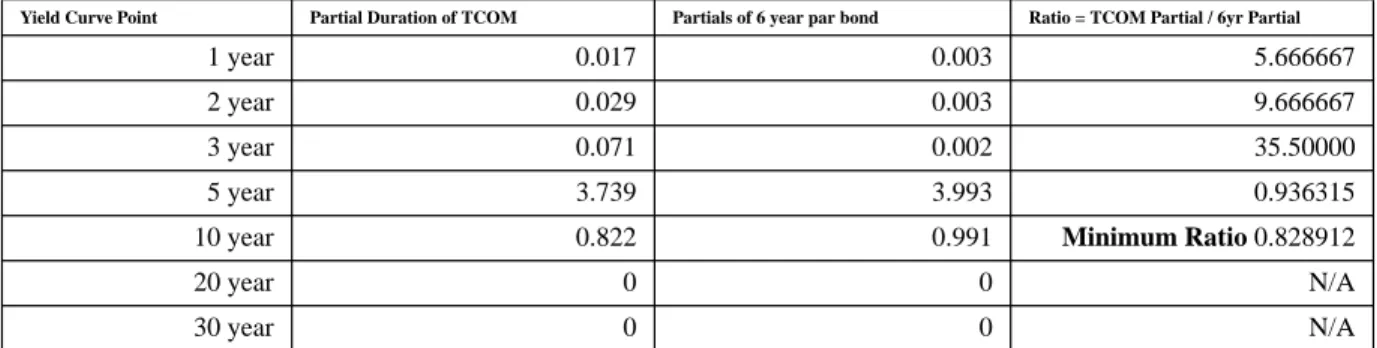
The data in the table comes from the circled fields in the picture on the opposite page.

Take the minimum ratio of the partial duration of the TCOM bond divided by the partial duration of the 6 year. This is the weight assigned to the best match bond; 82.9% of the MBP is the 6 year par bond.

Why take the minimum ratio?

If you used the amount indicated by the 5 year partial (93.6% of the 6 year), then the exposure to the 5 year would be .936 * 3.9931 = 3.738799, which is perfect, but the exposure to the 10 year would be .936 * .9913 = .927857 which is too high. The exposure of the bond at the ten year is only .8217. By taking the minimum of the ratios and then filling in the rest of the MBP, we do not have to create a more complicated MBP with short positions.

Solve for the rest of the MBP

The rest of the MBP consists of cash, 1, 2, 3, 5, 10, 20, and 30 year par Treasuries. The weights are calculated so that the MBP has the same effective duration and the same partial duration distribution as the secu-rity. The next page will take you through an illustration of this.

TABLE 1.Calculating the weight of the “best match” bond

Yield Curve Point Partial Duration of TCOM Partials of 6 year par bond Ratio = TCOM Partial / 6yr Partial

1 year 0.017 0.003 5.666667

2 year 0.029 0.003 9.666667

3 year 0.071 0.002 35.50000

5 year 3.739 3.993 0.936315

10 year 0.822 0.991 Minimum Ratio 0.828912

20 year 0 0 N/A

(18)

TCOM versus MBP

1 ₂

3

4

5

6

8

7

9

10

(19)

Methodology Example: TCOM versus MBP

In order to see that the MBP has the same partial duration exposure of the bond, we created a portfolio of user bonds representing the hypothetical treasuries in the MBP and set the par amounts equal to the weights as defined on the return attribution page. Let’s compare the partial durations of the TCOM bond to the MBP portfolio in Chapter 4.2.

AXP versus MBP: Partial Durations

STEP 1: Turn to Chapter 4.2, toggle <Buy> and click [Issue].

STEP 2: Type TCOM8,05 in the Ticker/Query field and click [Search].

Click the [B] in so it is yellow and enter a par amount.

STEP 3: Toggle <Sell> and click [Portfolio].

STEP 4: Enter “mtp” in the portfolio ID and click [Search].

Note: This portfolio is made up of the theoretical par bonds (user bonds) which were priced such that the yield was set equal to the par yield on the treasury model curve from 8/31/99.

STEP 5: Click on the portfolio to read it in.

STEP 6: Click [Pricing].

STEP 7: Toggle <Pricing Files> and click <Select>.

STEP 8: Click RA.Sep to retrieve the 8/31/99 pricing assumptions.

Remember that the partial duration matching used to calculate the MBP is based on the partial durations calculated from the beginning date of the return period.

STEP 9: On the Pricing Page, click Optional Calculations and select Risk

We must calculate Risk (partial durations) because user bonds are not in global price files. Remember global price files only contain “Salomon” source bonds.

(20)

Partial Duration Swap Report

11

12

13

14

Partial Duration difference is very close to zero.

The small differences is due to inaccuracies in constructing the MBP user bonds created for this example. The actual return attribution methodology matches the partial durations exactly.

(21)

Methodology Example: Scenario Analysis

STEP 11:Click [Report].

STEP 12:Click [Template Select].

STEP 13:Type “risk swap” in the yellow search field and click the glo-bal template RSKSWAP.

STEP 14:Click [Generate Report].

Methodology Example: Scenario Analysis

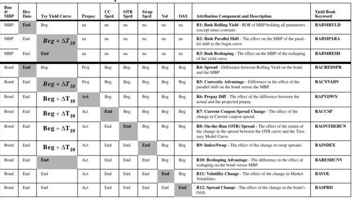
The next part of the methodology is the explanation of the successive sce-nario analyses that are run to calculate the attribution components. The table below shows the order of the scenario analysis. In each successive scenario calculation, one input is changed and one additional return attri-bution component is captured. The return input that is changed is shaded.

TABLE 2.Return Attribution Components Calculation

Bon d/ MBP

Hrz

Date Tsy Yield Curve Prepay CC Sprd

OTR Sprd

Swap

Sprd Vol OAS Attribution Component and Description

Yield Book Keyword

MBP End Beg na na na na na na R1: Bmk Rolling Yield - ROR of MBP holding all parameters

(except time) constant.

RABMRYLD

MBP End na na na na na na R2: Bmk Parallel Shift - The effect on the MBP of the

paral-lel shift to the begin curve

RABMPARA

MBP End End na na na na na na R3: Bmk Reshaping - The effect on the MBP of the reshaping

of the yield curve

RABMRESH

Bond End Beg Proj Beg Beg Beg Beg Beg R4: Spread - Difference between Rolling Yield on the bond

and the MBP

RACREDSPR

Bond End Proj Beg Beg Beg Beg Beg R5: Convexity Advantage - Difference in the effect of the

parallel shift on the bond versus the MBP.

RACNVADV

Bond End Act Beg Beg Beg Beg Beg R6: Prepay Diff - The effect of the difference between the

actual and the projected prepay

RAPYDWN

Bond End Act End Beg Beg Beg Beg R7: Current Coupon Spread Change - The effect of the

change in Current coupon spread.

RACCSP

Bond End Act End End Beg Beg Beg R8: On-the-Run (OTR) Spread - The effect of the return of

the change in the spread between the OTR curve and the Trea-sury Model Curve

RAONTHERUN

Bond End Act End End End Beg Beg R9: Index/Swap - The effect of the change in swap spreads. RAINDEX

Bond End End Act End End End Beg Beg R10: Reshaping Advantage - The difference in the effect of

reshaping on the bond versus MBP.

RARESHCNV

Bond End End Act End End End End Beg R11: Volatility Change - The effect of the change in Market

Volatilities

RAVOL

Bond End End Act End End End End End R12: Spread Change - The effect of the change in the bond’s

OAS. RASPRD Beg+∆T₁₀ Beg+∆T₁₀ Beg+∆T₁₀ Beg+∆T₁₀ Beg+∆T₁₀ Beg+∆T₁₀

(22)

Scenario Analysis

1

2

4 Relative

Shifts

3

5

6

7

8

(23)

Methodology Example: Scenario Analysis

The process we will go through in the following example is designed to illustrate the methodology and is similar to, but not the same as the pro-cess used within the Return Attribution Model. In the example, we will explain several of the return attribution factors by going through four sce-nario analysis calculations for the TCOM bond and its MBP.

STEP 1: Click [Scenario Setup] at the top of the Yield Book.

STEP 2: Click [Select] to display the list of scenario files.

STEP 3: Click retatwsn, which is a custom scenario file.

The default display shows the absolute rates of each scenario.

STEP 4: Toggle <Relative> to view relative shifts

The relative shifts are based on the settlement Yield Curve, the Treasury Model curve from the begin date, 8/31/99.

The first scenario is no change. The second is a parallel shift set equal to the amount that the ten year moved from 8/31/99 to 9/ 30/99 (down 5.6 bps). The ten year is the default for calculating the parallel shift. This can be customized by the user. The 3rd and 4th scenarios are set equal to the actual curve that existed on 9/30/99.

STEP 5: Click [Scenario Setup] to take the page down and click [ROR/CF] to bring up the Rate of Return Input Screen.

STEP 6: Define the horizon pricing method. Enter 5.9 as the OAS change in the 4th scenario for the TCOM security.

The horizon pricing method for the first three scenarios is con-stant OAS. The horizon pricing method for the fourth scenario is to change OAS by the amount the OAS changed on the bond from 8/31/99 to 9/30/99. In the example, the TCOM’s OAS went from a 103.4 to a 109.3 for an increase of 5.9bps.

STEP 7: Click [Calculate].

STEP 8: Toggle <Total ROR> and <Table>.

With these results, we can estimate the Return Attribution Com-ponents.

(24)

TCOM: ROR Results and Ret Att Detail

R4

_R1

R2

R3

R5

R10

R12

C A E D B

Scenario with final yield curve and constant OAS

(25)

Calculation of Components

Calculation of Components

The sequence of Scenario Analyses for return attribution follows the order as defined in the table on page 17. The ROR output can be labelled as shown below: (refer to labels in the ROR output picture on page 20).

R1 = ROR of MBP in no change scenario #1 (Benchmark Rolling Yld) =.529 R2 = ROR of MBP in parallel shift scenario #2 =.788

R3 = ROR of MBP in actual scenario #3 = .999

R4 = ROR of bond in no change scenario #1 (Total Rolling Yield) =.601 R5 = ROR of bond in parallel shift scenario #2 =.860

R10 = ROR of bond in actual scenario#4 with no OAS change = 1.071 R12 = ROR of bond in actual scenario#3 with OAS change =.798

Please note that the numbers produced by the illustrative methodology are close to but do not exactly match those produced by the actual model.

Benchmark Rolling Yield Component

The Benchmark Rolling Yield is the total return (ROR) on the MBP with a “no change” scenario, (R1) which is equal to .529

Spread Component The Total Rolling Yield on TCOM is the ROR on the bond in the “no change” scenario, (R4) which is.601. The Spread is equal to the Total Rolling Yield (R4) divided by the Benchmark Rolling Yield (R1) or:

Parallel Shift Component The parallel shift component is equal to the ROR of the MBP in the “par-allel” shift scenario (R2) divided by the ROR for the MBP in the “no change” scenario (R1) or:

Reshaping Component The reshaping component is equal to the ROR on the MBP for the “Actual” scenario (R3) divided by the ROR on the MBP for the “Parallel” shift scenario (R2) or:

Spread Change Component

The spread change component is equal to the ROR on the bond in the “Actual” scenario with an OAS change of 5.9 bps (R12) divided by the ROR on the bond in the “Actual” scenario at a constant OAS:

A (R1) B (R4/R1) 1.00601 1.00529⁄ –1 ( )×100 [ ] = 0.071621 C (R2/R1) 1.00788 1.00529⁄ –1 ( )×100 [ ] = 0.257637 D (R3/R2) 1.00999 1.00788⁄ –1 ( )×100 [ ] = 0.209350 E (R12/R10) 1.00798 1.010710⁄ –1 ( )×100 [ ] = –0.270107

(26)

FNMA 6.5

1

2 “Other”

Change in

Swaption

Volatility

(27)

Calculation of Components

Convexity Advantage The convexity advantage is equal to the difference in the effect of the par-allel shift on the bond (R5/R4) relative to the parpar-allel shift effect on the MBP (R2/R1).

Reshaping Advantage The reshaping component is equal to the difference in the effect of the reshaping on the bond (R10/R5) relative to the reshaping effect on the MBP (R3/R2).

Calculation of “Other” Attribution Components

Let’s return to the Return Attribution page and look at a mortgage bond to review the remaining “Other” attribution components (circled in the picture): volatility, prepay difference, current coupon spread, and OTR spread. Index/Swap is only calculated for floating rate securities.

Prepay Difference The effect of the difference between the actual and the projected prepays on the bond. This is only calculated for mortgages.

Volatility Change The effect of the change in market volatilities on the bond. For mort-gages, the important volatilities are the swaptions. Notice on the report on the left page that the 1 year option on the 10-year swap decreased from 16.4 to 15.10 (-1.3%) over the month. A decrease in vols causes the value of the option to decrease. Since you are short the option on the mortgage, this decrease in option value helps the mortgage; thus a posi-tive effect from volatility change of .228.

Current Coupon Spread Change

The current coupon spread change looks at the effect that the change in the current coupon spread has on the bond. The current coupon spread is the spread between the FNMA current coupon and the 10 year on-the-run treasury. For example, let’s look at the FNMA 6.5 bond in the ABCCo portfolio as shown on the opposite page.

STEP 1: Click on the FNMA 6.5 issue to bring up the Return Attribu-tion details of the bond.

STEP 2: Click [Print] to generate a return attribution report of just that one issue.

1.0086 1.00601⁄ 1.00788 1.00529⁄ ---–1    _×₁₀₀ ₌ _–_0.0002 1.01071 1.00860⁄ 1.000999 1.00788⁄ ---–1    _×₁₀₀ ₌ _–_0.0001

(28)

Current Coupon Spread

1

2

3

4

6

7

8

9

(29)

Current Coupon Spread

Overall, the mortgage had a spread advantage of 105.2 basis points. The current coupon spread was -.038 or -3.8 basis points. Let’s look at what happened to the current coupon spread over that period. You can also calculate a current coupon spread duration on the bond itself.

Current Coupon Spread

Turn to Chapter 2.2 and click [Hist Data] to go to Historical Data.

STEP 1: Click the white menu box next to A1 under the Security/ Issue label.

STEP 2: Toggle <Mortgages>.

STEP 3: Select FNMA Current Coupon.

STEP 4: Click on the white menu box next to A2 under the Security/ Issue label.

STEP 5: Toggle <Yield Curves> and select the 10 year (not pictured).

STEP 6: Click on the white menu box under the Equation label and select Spread.

STEP 7: Set the dates: From 8/31/99, To 9/30/99.

STEP 8: Determine which items you would like to display.

In this example, we clicked off the yields of the FNMA and the 10 year and said to display just the spread on the bottom.

STEP 9: Click [Graph].

For most mortgages, the current coupon spread duration is nega-tive, meaning that when the current coupon spread decreases, the value of the option to prepay increases which hurts the mort-gage (prices decrease). When the current coupon spread

increases, the value of the option is reduced which helps the mortgage (price increases). Here, the current coupon spread nar-rowed by 16 basis points from 165.5 on 8/31/99 to 149.5 on 9/ 30/99. This increases the value of the prepayment option; there-fore hurting the mortgage. The current coupon spread effect was a negative 3.8 bps which hurt the return.

(30)

(31)

On-the-Run Spread The On-the-Run spread is the effect of the return of the change in the spread between the OTR curve and the Treasury Model Curve. First, lets look at the table of information below:

The first two columns of numbers come from the Curve Analysis page as shown on the opposite page. The third column is simply the difference of the first two columns. The fourth column comes from the analysis we did on the current coupon spread on page 24.

The current coupon spread effect is calculated by looking at the spread between the FNMA current coupon and the On-the-Run 10 year treasury. Now we are looking at the spread between the FNMA current coupon and the Treasury Model 10 year point. This spread is equal to the CC spread minus the Spread between the 10 year OTR and Treasury Model points as shown:

From the table above, we compute this spread to be: = -16 - 3.5 = -19.5 bps.

The spread between FNMA current coupon and Treasury Model nar-rowed by 19.5 bps (versus a narrowing of only 16bps between the FNMA and the 10 year On-the-Run. As discussed above in the Current Coupon Spread, a narrowing of this spread hurst the mortgage. The effect of this 3.5 bps additional narrowing should hurt the mortgage even more. This is shown in the OTR Spread change value of -.007.

Date 10 year OTR 10 Year Treasury

Model

Spread between OTR and Treasury Model Current Coupon Spread 8/31/99 5.983 6.291 30.8 165.5 9/30/99 5.893 6.236 34.3 149.5 Change 9 bps 5.57 bps +3.5 bps -16bps

(32)

Portfolio Level Attribution: Report

1

2

3

4

5

(33)

Generate the Portfolio Level Attribution Report

The individual bond attribution components are averaged using the IRR method (which will be explained in the next section) to compute the port-folio average measures.

To generate portfolio reports instead of individual bond reports, do the following:

STEP 1: Click [Report].

STEP 2: Click [Template Select].

STEP 3: Enter “return att” in the yellow search field.

STEP 4: Click on Retatt02, the report of ROR components for each bond and the average.

STEP 5: Click [Generate Report].

The report displays each of the components and the total return for the period. In addition, the summary levels, TOT TSY for Total Benchmark and TOT SPD ADV for Total Spread Advan-tage are given. Please see the circled columns on the opposite page.

Note: Use the return attribution sector template (RETSEC1 or RETSEC2) and a sector file to generate the return attribution components by sector.

(34)

Introducing Dynamic Portfolios

Static vs. Dynamic Portfolios

In a static portfolio where all securities are invested for the entire analysis period, the portfolio average return (and return components) can be derived by calculating the market weighted average return(s) across all securities. This is not true for a dynamic portfolio, which has transactions as well as cash inflows or outflows.

Viewing a Portfolio as a Collection of Investment Segments

An investment segment is a holding in a security from Time A to Time B. If a security is in the portfolio throughout the analysis period, Time A is the beginning of the analysis period and Time B is the end of the analysis period. If a security is purchased and sold within the analysis period, Time A is the purchase trade date and Time B is the sell trade date.

Transactions: Assumptions about Investment Segments

For active portfolios, you will define the portfolio composition at the beginning of the analysis period and all of the transactions (buys, sells, cash inflows, cash outflows) over the period. The Yield Book will pre-process the beginning portfolio and transactions into investment seg-ments. The details of how to enter transactions and which type of cash inflows and outflows must be entered versus which are assumed to have occurred by the system will be defined in the next section with examples. In this section, we wish to explain how portfolio averages are calculated for dynamic portfolios.

IRR Method for Averaging Returns

For example, we want to analyze the performance of a portfolio over the month of August, 1998. On July 31, 1998, the portfolio consists of 5 mil-lion par in each of 3 securities: a treasury, a corporate, and a mortgage. On August 15, the corporate is sold and the proceeds are reinvested in the treasury security.

This portfolio in the month of August will consist of 4 investment seg-ments:

Investment Segment Security Time A Time B

1 Treasury 7/31/98 8/31/98

2 Mortgage 7/31/98 8/31/98

3 Corporate 7/31/98 8/15/98

(35)

The IRR Method for Averaging Returns

The IRR Method for Averaging Returns

The first step is to calculate the total return and return attribution compo-nents for each investment segment as described in the methodology sec-tion of this manual.

The portfolio return (and return components) can be averaged via an Internal Rate of Return (IRR) calculation. The IRR method is an AIMR Standards approved method for calculating time weighted rates of return. Its primary advantage is that it does not require the definition of market values for the static securities in the portfolio on the days of transac-tions, cash inflows, and cash outflows. For this reason, you only need to define the trade price of the bonds you trade on the transaction dates, not all the remaining static securities.

The basic calculation is: find R such that:

where,

Mi= Market Value (beginning) of investment segment i

R_i = Return of Investment Segment i R = Internal Rate of Return

ti1 = Start time (between 0 and 1) for investment segment i

t_i2 = End time (between 0 and 1) for investment segment i

In a static portfolio where all investment segments span the entire analy-sis period, the IRR will equal the Market Weighted Average Return.

Applying the IRR Method to Averaging Return Attribution Components

The attribution components for each investment segment are calculated through a series of scenario analysis return calculations on the security or its Matched Benchmark Portfolio (MBP). The scenario analysis returns are cumulative. That is, in each scenario analysis run, an additional factor is introduced. To calculate the return effect of any of the 12 factors, the first scenario return which includes that factor, is divided by the prior sce-nario return. The total return for the investment segment is the return of the 12th scenario analysis run (in which all 12 factors are reflected) which, by definition is the product of the 12 Return Attribution Compo-nents.

M

∑

i

(

1 +

R

i

)

1 +

R

(

)

ti2

---

M

i

1 +

R

(

)

ti1

---∑

=

(36)

The portfolio average for each of the 12 return attribution components can be computed through a two-step process. First, calculate the IRR for each of the 12 cumulative scenario returns. The portfolio average for each attribution component can then be calculated by successively divid-ing the cumulative IRRs.

Examples

The following three examples will illustrate the IRR calculation for static and dynamic portfolios. In order to simplify the examples, we will con-solidate the 12 return components into 2 major return categories:

Bench-mark Return which is the product of the BenchBench-mark Rolling Yield,

Parallel Shift and Reshaping components, and the Spread Advantage which is the product of all the remaining components.

Example 1: Static Portfolio

The following table displays the returns and major attribution compo-nents for each segment of XYZCO over the month of August, 1998. Since this is a static portfolio, the average returns can be calculated using a simple market weighted average method, but we will show the IRR method for example:

Step 1: Calculate Portfolio Benchmark Return

Using the IRR equation,

and since t_i2= 1 and t_i1= 0 for all i, we solve for R such that

R =.02640 and Portfolio Benchmark Return = 2.640%

Segment Security Beg Par Beg Mkt (Mi) ti1 ti2 Bmk ROR (Ri) Spread Adv Total Return

1 US 5000 5594 0 1.0 3.010 -0.005 3.004 2 TCOM 5000 5280 0 1.0 3.379 -3.444 -0.181 3 FNMA 5000 5112 0 1.0 1.472 -.560 .904

M

∑

i

(

1 +

R

i

)

1 +

R

(

)

ti2

---

M

i

1 +

R

(

)

ti1

---∑

=

5594 1.0301( ) 1+R ( ) --- 5280 1.03379( ) 1+R ( ) --- 5112 1.01472( ) 1+R ( ) ---+ + = 5594+5280+5112

(37)

Examples

Step 2: Calculate Portfolio Total Return

The portfolio Total Return is solved for using the same equation. Just substitute the Total ROR numbers in place of the Benchmark Return numbers in the above formula and solve for R:

R =.01281 and Portfolio Total Return = 1.281%

Step 3: Calculate Portfolio Spread Advantage Return

The portfolio Spread Advantage Return is calculated by dividing the Total Return by the Benchmark Return:

Portfolio Spread Advantage = (1.01281/1.0264 -1) x 100 = -1.324%

Important Note: The IRR Method on the other hand, is designed to maintain the cumula-tive property of the returns so that the product of the component averages will equal the total return average.

Example #2: Dynamic Portfolio

In this example, we will introduce transactions in the XYZCO portfolio. We will assume that the holdings in the TCOM and FNMA securities were sold on 8/20/98 and all proceeds (including cash generated during the period) were reinvested in the Treasury security.

Step 1: Define Investment Segments for XYZCO Portfolio in August 1998

The portfolio would contain 4 investment segments. The market values, par amounts, and returns are shown below:

Step 2: Calculate Portfolio Benchmark Return

Using the IRR equation, we solve for R such that

this results with R=.02923 and Portfolio Benchmark Return = 2.923% 5594 1.030040( ) 1+R ( ) --- 5280 0.9982– 1+R ( ) --- 5112 1.00904( ) 1+R ( ) ---+ + = 5594+5280+5112

Segment Security Beg Par Beg Mkt (Mi) ti1 ti2 Bmk ROR (Ri) Total Return

1 US 5000 5594 0 1.0 3.010 3.004 2 TCOM 5000 5280 0 .667 1.255 .236 3 FNMA 5000 5112 0 .667 .658 .394 4 US 9519 10425 .667 1.0 1.903 1.910 5594 1.03010( ) 1+R ( )1 --- 5280 1.01255( ) 1+R ( )0.667 --- 5112 1.00658( ) 1+R ( )0.667 --- 10425 1.01903( ) 1+R ( )1 ---+ + + 5594 1+R ( )0 --- 5280 1+R ( )0 --- 5112 1+R ( )0 --- 10425 1+R ( )0.667 ---+ + + =

(38)

Step 3: Calculate Portfolio Total Return

Calculate Portfolio Total ROR using the same equation as above except substitute the Bmk Return (R) with the Total Return (R) from the table above. This results with portfolio Total Return of 2.501%

Step 4: Calculate Portfolio Spread Advantage

The portfolio Spread Advantage is calculated by dividing the Total Return by the Benchmark Return.

Portfolio Spread Advantage = (1.02501/1.02923-1) x 100 = -0.410% The Benchmark Return in a dynamic portfolio is higher than for the static portfolio due to the fact that the 8/20/98 transaction increased the dura-tion of the portfolio.

(39)

Allocation of Returns to Sector and Issue Level Components

Allocation of Returns to Sector and Issue Level

Components

Once the individual and portfolio level attribution is completed, you may wish to allocate either the total return or just the total spread advantage component to either issue or sector selection. To allocate return into sec-tor and issue level components, you must choose a benchmark, usually an index. You can allocate total return (relative to the index) or just the total spread advantage return (relative to the index) to either issue or sector selection. The allocation equations are shown below.

Sector Weighting in Sector

(Index Return in sector - Total Index Return) * (Portfolio Overweight in sector)

Issue Selection in Sector (Portfolio Return in sector - Index Return in sector) * (Sector Weight of Portfolio)

• Note: The basic allocation of return into sector and issue level

compo-nents is usually done on the Spread Advantage Return (relative to the index), which is the return after the treasury effects (duration and yield curve reshaping) are broken out. Some users may wish to allocate the Total Return (relative to the index) into Sector and Issue level compo-nents including the treasury portion. The compocompo-nents for each of these methods are shown on the following page.

(40)

Return Attribution Major Components

Total Return

Subtract Index

Total Return

Difference

Sector Effect

Difference

Issue Selection

Difference

Total

Return

Spread Return Advantage Treasury Return Subtract Index Treasury Return Subtract Index Spread Advantage Return Spread Advantage Return Difference Duration and Yield Curve Difference Sector Effect Difference Issue Selection Difference Total Return Difference

=

+

Allocation of Total Return of a Portfolio with an Index Benchmark

(41)

Allocation of Returns to Sector and Issue Level Components

The objective is to allocate the portfolio’s total return (relative to the index) into three major categories, corresponding to the three major steps in the portfolio management process.

Steps in the Portfolio Management Process for Single Currency

Portfolios

STEP 1: Define the total portfolio duration and yield curve exposure.

STEP 2: Define the weight in each sector. The weighting decision can be broad (mortgage vs. corporate vs. treasury) or narrow (utility, industrial, GNMA, FNMA, etc).

STEP 3: Select specific issues within each sector.

The attribution attributed to Step 1 is the average Treasury Return (rela-tive to the index) for the portfolio. The balance of the portfolio return is the Spread Advantage. The Spread Advantage is decomposed into Sector Weighting components for each sector (capturing the return attributable to Step 2 above) and into Issue Selection components (returns attribut-able to Step 3). Select Portfolio Duration and Yield Curve Exposure Select Sector Weights Select Specific Issues

Step 1 Step 2 Step 3

(42)

Sector and Issue Level Attribution: Example #1

1

2

5

6

7

8

3

4

(43)

Examples: Sector and Issue Allocation

Examples: Sector and Issue Allocation

The Yield Book allows great flexibility in defining the sectors to be used in Sector Level Attribution. The Sector Weighting and Issue Selection components depend on the number of sectors used. In the extreme, if there is only one sector, all of the Spread Advantage is allocated to Issue Selection. In the other extreme, if every security is in a different sector, all of the Spread Advantage is allocated to Sector Weighting.

It is very important that you define your sectors based on your portfolio decision making process. In the next two examples, we will apply two different sector files to the ABCco versus the BIGINDEX and you will notice that the results tell a very different story depending on the sector breakdown that is used.

Example#1: ABCco vs. BIGINDEX broken down by THREE major industry sectors

Compare the ABCco portfolio to the BIGINDEX as of 9/1/99.

STEP 1: Toggle Buy in Ch 4.6 and click [Portfolio] and click ABCco as of 9/1/99.

STEP 2: Toggle Sell in Ch 4.6 and click [Portfolio], toggle Indexes and click BIGINDEX 9/1/99.

STEP 3: Click [Read Results] and select RA.SEPT (not pictured).

STEP 4: Click [Report] to obtain the template selection page.

STEP 5: Type “bmk” in the yellow template search field.

STEP 6: Select RETBMK template.

STEP 7: Click [Sector Select] and choose a sector.

In this example, we selected a sector file called “MAJOR” which is made up of three sectors:

Treasury or Agency, Mortgage, and Corporate

(44)

Sector and Issue Selection: Example #1

Corporate

Mortgage

Treasury

(45)

In order to calculate the issue and sector selection, you must have the market weights in each of your sectors for the portfolio and for the index as well as the total spread advantage in each of your sectors for the port-folio and for the index. These are taken from the report shown on the opposite page and summarized in the tables below:

Sector Selection Effect:

Issue Selection Effect:

Total:

Sector Weighting

in Sector

=

Index spreadadvantage in sector Total Index spread. advantage Portfolio Overweight X in sector

col 1 col 2 col 3 = col 1-2 col 4 col 5 col 6 = col 4- 5 col7 = col3*6/100

Sector Market Weight Portfolio Market Weight Index Over or Under Weight Spread Advantage Index Sector Spread Advantage

Total Index Difference

Sector Weight Effect Tsy/Agn 38.18 44.63 -6.46 .125 .394 -0.269 .017377 Mortgage 34.69 32.03 2.65 .906 .394 .512 .013568 Corporates 27.14 23.33 3.81 .207 .394 -0.187 -.007125 Total 100 .023820 Issue Selection in Sector

=

Portfolio spread advantage in sector Index spread advantage in sector Sector Weight of Portfolio X

col 1 (from above) col 8 col 4 (from above) col 9 = col 8 - 4 col 10 = (col1*col9)/100

Sector Market Weight Portfolio Spread Advantage: Portfolio Sector Spread Advantage:

Index Sector Difference Issue Selection Effect

Tsy/Agn 38.18 -0.013 .125 -0.138 -0.051848

Mortgage 34.69 1.052 .906 .145 .050301

Corporates 27.14 -0.048 .207 -0.254 -0.068936

Total 100 -0.070483

Sector

Sector Weight Effect (col 7 from above)

Issue Selection Effect

(col 10 fro above) Total Effect

Tsy/Agn .017377 -0.051848

Mortgage .013568 .050301

Corporates -.007125 -0.068936

(46)

(47)

Example#2: ABCco vs. BIGINDEX broken down by FOUR major industry sectors

Let’s say you don’t manage your Treasury/Agency allocation as one unit, but as two separate sectors. We will use a new sector file that had four sectors:

Treasury, Agency, Mortgage, and Corporate

Regenerate the report with the new sector and review the results. Details of how the numbers are calculated are shown in the tables on the next page.

Remember, you can customize the sectors that you report on by editing or creating sector files in Chapter 1.5.

(48)

Example #2: Treasury and Agency Broken Down

Sector Selection Effect:

Issue Selection Effect:

Total:

col 1 col 2 col 3 = col 1-2 col 4 col 5 col 6 = col 4-5 col 7 = col3*col6/100

Sector Market Weight Portfolio Market Weight Index Over or Under Weight Spread Advantage : Index Sector Spread Advantage Total

Index Difference Sector Weight Effect

Treasury 38.18 34.05 4.13 -0.0002 .394 -0.3942 -0.01628

Agency 0 10.58 -10.58 .534 .394 .14 -0.014812

Mortgage 34.69 32.03 2.65 .906 .394 .512 .013568

Corporate 27.14 23.33 3.81 .207 .394 -0.187 -0.007125

Total -0.024649

col 1 (from above) col 8 col 4 (from above) col 9 = col 8 - 4 col 10 = (col1*col9)/100

Sector Market Weight Portfolio Spread Advantage: Portfolio Sector Spread Advantage:

Index Sector Difference Issue Selection Effect

Treasury 38.18 -0.013 -0.0002 -0.010 -0.003818 Agency 0 0 .534 -0.534 0 Mortgage 34.69 1.052 .906 .145 .050301 Corporates 27.14 -0.048 .207 -0.254 -0.068936 Total 100 -0.022453 Sector

Sector Weight Effect (col 7 from above)

Issue Selection Effect

(col 10 from above) Total Effect

Treasury -0.01628 -0.003818

Agency -0.014812 0

Mortgage .013568 .050301

Corporates -0.007125 -0.068936

(49)

Comparison of Sector Weight and Issue Selection

Comparison of Sector Weight and Issue Selection

Now we can compare the allocation between sector and issue under the two sector files:

Table #1 with Three Sectors

Table #2 with Four Sectors (Agency separate)

Notice that in Table #1 using just three sectors, it looks like the decision to overweight Treasury/Agencies was a good sector decision, but you picked poor issues. In Table #2, it shows us that to have overweighted Treasuries and to have underweighted Agencies were both bad decision. This would only be found by breaking the Agency sector out.

Sector Sector Weight Effect Issue Selection Effect Total Effect

Tsy/Agn .017377 -0.051848

Mortgage .013568 .050301

Corporates -.007125 -0.068936

Total .023820 -0.070483 -0.046663

Sector Sector Weight Effect Issue Selection Effect Total Effect

Treasury -0.01628 -0.003818

Agency -0.014812 0

Mortgage .013568 .050301

Corporate -0.007125 -0.068936

(50)

(51)

WORKSHOP

Salomon Analytics Inc.

Return Attribution: Examples

Agenda

This section of the advanced capabilities handbook takes you through several return attribution exam-ples to illustrate the inputs and outputs of the return attribution model.

Highlights

In this workshop handbook, we will cover Return Attribution examples that teach the following:

• How to use Salomon Smith Barney (SSB) pre-calculated results for return attribution. • How to combine Index pricing and User pricing, where difference between the Index

and User pricing is captured as an additional attribution component called User price adjustment.

• How to enter Duration and Prepayment Overrides to bonds.

(52)

2-2 Return Attribution: Examples

Example #1: Static Portfolio using SSB Pricing

1

2

3

(53)

Return Attribution Implementation: Examples

Return Attribution: Examples 2-3

Return Attribution Implementation: Examples

The most important thing to do before starting to run return attribution is to decide what pricing to use for bonds that SSB provides pricing on.

Three Choices about Pricing

1. Use the SSB price in your total ROR calculation and the attribution calculation. (Example #1 below)

2. Use your own price for the total ROR calculation and the attribution calculation (Example #2-Part A below)

3. Use your own price for the total ROR calculation and the SSB price for the attribu-tion calculaattribu-tion. This is the most commonly used method because you save time on the attribution calculation by using the pre-calculated results and you are able to report actual returns using your own prices. (Example #2-Part B below)

This decision determines the sequence in which you perform your calcu-lations and the steps required.

Example #1: Static Portfolio using SSB Pricing

Problem Assumptions: You wish to use Salomon Smith Barney (SSB) provided Prices for all available bonds. For bonds that SSB does not provide a price, you will use your own user prices. These user prices can be entered either manu-ally using the pricing page or loaded from a pricing file. This example will show the manual method. Using user price files will be shown as part of Example #2.

STEP 1: Turn to Chapter 4.6, Toggle <Buy> and click [Portfolio].

STEP 2: Select the portfolio ABCco2 from the listbox.

STEP 3: Click [Read Results].

STEP 4: Click RA.SEP

What is a Results File? A result file is composed of the return calculation, the attribution compo-nents as well as the beginning and ending price files including the partial durations of all the bonds. When you read in a results file, everything is restored to the parameters used when the calculation was completed. Notice in the page status section that there is one unpriced bond for the beginning and ending dates. On the following page we will focus in on this bond and price is manually.

(54)

5

7

6

8

10

9

(55)

Example #1: Static Portfolio using SSB Pricing

STEP 5: While toggled on <Buy>, click [Focus] to bring up the Focus Selection page.

STEP 6: Click RETATT04, a predefined sector condition that focuses on unpriced securities.

STEP 7: Click [Process].

The one unpriced bond, FMCR, is the only bond focused in. Note: Since this sample portfolio is small, it would have been easy to locate the unpriced security without using the focus step. In a large portfolio, it is more difficult to locate the unpriced securities, and requires the focus capability.

STEP 8: Click [Pricing Page].

STEP 9: Enter a price of 102 (the begin price) in the new level column for the FMCR bond.

STEP 10:Click [Update Buy Prices].

Make sure that if you are pricing a mortgage that you are using the SSB prepayment model in order to calculate an OAS and Effective Duration. (Note: For a CMO, the CMO OAS/EDUR option box must also be turned on).

The calculation of the partial durations required for the MTP calculation do not have to be calculated at this point; therefore the RISK option under Optional Calculations need not be on at this time. When the return attribution calculation is run, the risk measures are automatically calculated.

(56)

11

12

13

14

15

(57)

Example #1: Static Portfolio using SSB Pricing

STEP 11:Toggle <End>.

We must also provide a price for the end date.

STEP 12:Enter a price of 103 in the new level column for the FMCR bond.

STEP 13:Click [Update Buy Prices].

STEP 14:Click [Unfocus].

Notice in the page status that one bond still needs calculations.

STEP 15:Toggle on <Ret Att> under the calculations section and Click [Calc Ret Att].

Summary: In this example #1, we used the pre-calculated results from the Return Attribution results file for all bonds which SSB provides a price. For the one user bond, FMCR, we had to enter begin and end user prices and cal-culate the return and attribution components. The results are:

Review of Decision about Pricing

In most cases when running Return Attribution on your portfolios, you will own some combination of bonds that we have pre-calculated results for and some bonds that we do not have pre-calculated results for. When SSB does not provide pricing and pre-calculated results, it is obvious that you must use your own prices and calculate results for those bonds. When SSB does provide pricing and attribution results for all of your bonds, you have the three choices on what pricing and attribution results to use, see “Three Choices about Pricing” on page 3.

Total Rate of Return 1.233

Treasury Return .828

(58)