Incorporating Cloud Distribution in Sky Representation
Kuan-Chuan Peng, Tsuhan Chen
Cornell University
Ithaca, NY, USA
{kp388, tsuhan}@cornell.eduAbstract
Most sky models only describe the cloudiness of the over-all sky by a single category or parameter such as sky index, which does not account for the distribution of the cloud-s acrocloud-scloud-s the cloud-sky. To capture variable cloudinecloud-scloud-s, we extend the concept of sky index to a random field indicating the lev-el of cloudiness of each sky pixlev-el in our proposed sky repre-sentation based on the Igawa sky model. We formulate the problem of solving the sky index of every sky pixel as a la-beling problem, where an approximate solution can be effi-ciently found. Experimental results show that our proposed sky model has better expressiveness, stability with respect to variation in camera parameters, and geo-location esti-mation in outdoor images compared to the uniform sky in-dex model. Potential applications of our proposed sky mod-el include sky image rendering, where sky images can be generated with an arbitrary cloud distribution at any time and any location, previously impossible with traditional sky models.
1. Introduction
Have you ever taken photos outdoors and wished to ma-nipulate the clouds such that the photos will look better? Have you ever imagined transferring the cloud distribution from one image to another to reflect the change of geo-location and time? Such applications require a sky rep-resentation that includes the clouds. Ideally, a sky model should consider different weather conditions, the cloud dis-tribution, the scattering of the sunlight, and so on. Such a complete sky model has not yet been proposed. In this paper, we propose a sky model that incorporates a cloud distribution, which is a step towards this ideal sky model.
In recent decades, researchers in atmospheric science and related fields have proposed different sky models to fit the measured luminance or radiance of the sky. One major class of those models classifies the sky into one of the sev-eral predefined categories from clear to overcast, including the Perez sky model [15] and the CIE standard sky model
Figure 1. An example of our proposed sky representation. The upper image is the input sky image (from [19]). The lower image is its sky index image in our model, where more brightness indicates less cloud density.
proposed by Kittler [10]. Those sky models limit the types of appearance of the sky, and the concept of cloudiness in those models is a discrete-level general representation for the overall sky. In other words, the cloud distribution is implicitly assumed to be uniform, which is not an accurate representation of the real world.
In computer vision, several applications leverage the in-formation provided by the sky. Lalonde et al. [11, 12] esti-mate camera parameters and natural illumination condition-s, and geo-locate outdoor images by the sky appearance as well as the detected sun position. Jacobs et al. [9] also esti-mate the camera parameters with the luminance of the sky by normalized cross correlation. However, the above works use additional algorithms or manual selection to ensure that the sky should be clear in the outdoor image. The reasons are twofold: First, using sky images with clouds requires additional complexity in algorithm design and implementa-tion. Second, existing sky models encourage researchers to use sky images where the clouds are uniform, making clear sky images the easy choice.
Modeling clouds is also a popular topic in comput-er graphics. Schpok et al. [17] use qualitative cloud at-2013 IEEE International Conference on Computer Vision
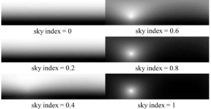
Figure 2. Sample sky maps generated by the Igawa sky model. The horizontal axis is azimuth angle (0 to 360 degrees from left to right), and the vertical axis is altitude from horizon to nexus (0 to 90 degrees from bottom to top). Sky index ranges from 0 (over-cast) to 1 (clear) representing the degree of cloudiness. In this case, the solar azimuth and altitude are 90 and 30 degrees respec-tively. Each sky map is scaled between 0 (black) and 1 (white) for display.
tributes to generate a volumetric cloud model. Hufnagel and Held [6] summarize recent cloud models in three aspect-s: cloud representation, rendering techniques, and lighting techniques. Even though using some of the cloud models can produce realistic sky images, most of these cloud mod-els do not take the geo-location and timestamp into con-sideration. Further, these rendering models are not used to represent a sky from an actual image, as is our goal.
In this paper, we propose a sky representation based on the Igawa sky model [7], which is shown to fit better to the real measured data than other existing sky models, in-cluding models proposed by Perez [15], Brunger [2], Har-rison [4], and Kittler [10]. In the Igawa sky model, a sky index is introduced as a model parameter describing the cloudiness of the overall sky. We extend the concept of sky index to every sky pixel location to capture the cloud dis-tribution. The proposed sky representation is demonstrated in Figure 1, where the sky indices are normalized such that the whiter the pixel in the sky index image is, the clearer that sky pixel is. Lalonde et al. [12] also estimate the cloud-s and cloud-sky turbidity by cloud-solving the weight acloud-scloud-signed to each pixel, where the weight is not directly linked to some phys-ical model and a data-driven prior model is needed for clear skies. Our model only uses an image and the Igawa sky model to estimate the sky indices which have direct phys-ical interpretation [7]. Li et al. [13] proposed a thin cloud detection algorithm using Markov random fields, but their binary labeling algorithm can only handle images with thin clouds. Our model not only accepts various types of clouds in the input image but utilizes the geo-location and a physi-cal model, which is not considered in [13].
We make the following contributions: 1: we extend the
uniform sky index model on having a per-pixel sky index that accurately represents cloud distributions. 2: we show applications of our sky index map for sky re-rendering and geo-localization from a single image of the sky.
2. Igawa sky model
In this paper, we assume that the intensityI(si)of any sky pixelsi obeys the distribution of the Igawa sky mod-el [7] according to the following function:
I(si)∝Lez(γs)·φ(π/2)φ(γ·)f·(fπ/2(ζ)−γ
s), (1) whereLez(γs)is the zenith radiance,γ(γs) is the altitude of the sky pixel (sun) in radians, andζis the angular dis-tance between the sun and the sky pixel. φ(·)(gradation function) andf(·)(scattering indicatrix function) are both functions of sky indexSi, which is a real value between 0 (overcast) and 1 (clear) representing the degree of cloudi-ness. The concept of sky index in the Igawa sky model is only defined globally for the entire sky, not for any partic-ular pixel. In our algorithm, we extend the concept of sky index to every sky pixel to generate one sky index per pixel. In this paper, we use the term “sky maps” for the simu-lated sky images generated by the Igawa sky model and use them to estimate the camera parameters (zenith, azimuth, and focal length) when solving for sky indices. Figure 2 demonstrates the sample sky maps under the condition that solar azimuth equals 90 degrees and solar altitude equals 30 degrees with variousSi.
3. Problem formulation
Our goal is to find the sky indices of all the sky pixel-s that bepixel-st reproduce the pixel-sky image. We begin by intro-ducing the notation used in this paper. Consider a random field of sky indicesSIdefined over the set ofnsky pixels
S and a neighborhood systemN. Each sky pixelsi ∈ S has a random variableSIi ∈ SI, indicating its sky index value. Assume there aremevenly separated discrete lev-els of sky indices andSIitakes a value from the label set
L={l1, l2,· · ·, lm}whereli = mi−−11. A possible assign-ment of labels to allSIiis defined as a labelingl∈Ln. Our goal is to find a labeling to minimize the following energy functionE(l): E(l) = si∈S ψi(SIi) + si∈S,sj∈N(si) ψij(SIi, SIj) (2) whereN(si)is the set of neighboring sky pixels ofsi. The unary term ψi ensures the sky index of each sky pixel is consistent with the observed dataI(si)under the Igawa sky model. The binary termψijpromotes sky index smoothness by encouraging neighboring sky pixels to take similar sky indices. We defineψiandψijin Sec. 4.
Figure 3. The flowchart of the algorithm solving the sky indices in our proposed model for all the sky pixels.
4. Calculating the sky indices
To solve the sky index for each sky pixel, we propose an algorithm shown in Figure 3. We hypothesize a set of sky images that are used to initialize the sky index, and we perform inference to optimize Eq. (2) with this initializa-tion. Given a geo-located input image with timestamp, we first compute the exact solar zenith θs and solar azimuth
φsby [16] and feed the sun orientation and the timestam-p as the intimestam-put of the Igawa sky model to generate a series of sky maps under mlevels of sky indicesl1, l2,· · ·, lm. Second, assuming that the camera parameters are not giv-en as input and that the camera has no roll angle, we need to estimate camera zenith θc, camera azimuthφc, and fo-cal lengthf while solving the sky indices for all sky pixels. Therefore, we sample a set of triple (θc, φc, f). For each hypothesis, we calculate the normalized cross correlation valueNCC(si, lj)between the image patch aroundsiand the corresponding patch in the sky map usingljas sky index for every sky pixelsiand all possiblelj ∈L. The hypoth-esis that maximizesg(S, SI)provides the estimated values for(θc, φc, f), where
g(S, SI) =
si∈S
NCC(si, SIi). (3) The sky index SIi for each Si is initialized as the value
lj ∈ L that maximizesg(S, SI). Given the initial values for allSIi, we useα-expansion algorithm [1] to minimize
E(l)in Eq. (2) because it can efficiently provide a solu-tion guaranteed to have certain closeness to the optimal one. Givenθs,φs,θc,φc,f, andSI, we reconstruct the sky im-age by retrieving the corresponding intensities in sky maps (Figure 4).
The unary termψiused in our algorithm is written as:
ψi(SIi) =c1−NCC(si, SIi) +c2|Ir(si)−In(si)|,
(4) wherec1andc2are constants. The last term corresponds to the reconstruction error, whereIr(si)is the normalized in-tensity ofsiin the reconstructed sky image generated by the Igawa sky model with currentSI, andIn(si)is the normal-ized intensity ofsiin the input sky image. We use L1-norm
Figure 4. The flowchart of the algorithm reconstructing the sky image from the corresponding sky index image.
in the last term of Eq. (4) because we want to penalize every unit of difference equally. We also try L2-norm in Eq. (4) and it produces similar results. The constantsc1andc2are chosen such that the two parts of the unary term have com-parable ranges.
A contrast sensitive Potts model is used for the binary termψij:
ψij(SIi, SIj) =
0 ifSIi=SIj,
h(i, j) otherwise, (5) andh(i, j)is a function based on the difference of colors of neighboring pixels with the following form:
h(i, j) =c3+c4·exp
−c5· Ic(si)−Ic(sj)2
, (6) where c3, c4, and c5 are constants chosen empirically.
Ic(si)andIc(sj)are the color vectors of pixelsi andsj respectively. In our experiment, the model parameters we used are (c1, c2, c3, c4, c5) = (1,1,0.1,0.1,1). Figure 6 demonstrates the result of our algorithm usingm= 11with the sample images in column (a). Column (b) and (c) are the
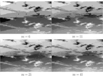
Figure 5. The sky index images and the corresponding reconstruct-ed sky images using different numbers of discrete sky index levels mwith the same input sky image as that in Figure 1. In each case ofm, the top image is the solved sky index image where brighter pixels indicate clearer sky, and the bottom one is the reconstruct-ed sky image where brighter pixels represent higher intensity. A largermproduces finer reconstructed images.
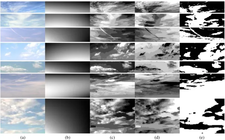
reconstructed sky images generated by the flow in Figure 4 with the uniform sky index model and our proposed model respectively. As the estimated sky index images solved by the flow in Figure 3, column (d) is used to generate images in column (c). Column (c) is not just the negative images of column (d) because two pixels with the same sky index may have different intensities in the reconstructed image. Column (e) is the results of thin cloud detection by [13] where white (black) pixels represent clouds (sky). Qualita-tively, our model captures the cloud distribution better than either the uniform sky index model or Li’s method [13]. In Figure 6, we only show the portion of the sky (our region of interest), and the sky index images are shown such that brighter pixels indicate clearer sky. We reconstruct the sky images only in gray scale because the Igawa sky model only defines the radiance distribution of the sky. The chromatic information is related to the scattering of the sunlight, which will complicate our current model. The sky index images is finer whenmincreases, which is shown in Figure 5. For computational efficiency, we usem = 11in our experi-ment. The image of sky indices and reconstructed images are normalized to enhance the contrast for display.
4.1. Limitation of the proposed model
There are some cases such that the sky index images de-termined by the algorithm of Figure 3 are inconsistent with a human’s perception. Figure 7 shows some typical failure cases from the AMOS data set [8]. The intensities in the areas marked by the red rectangles in column (d) should be darker than the solved values. In other words, some
over-cast pixels are incorrectly labeled as clear. This is unfor-tunate but expected because the Igawa sky model does not have volumetric concept of the clouds, and some physical phenomena (such as the shadows, the scattering of the sun-light, and reflection and refraction) within the clouds are not fully modeled. If an overcast pixel happens to have similar appearance as that of a clear pixel and the normalized cross correlation between the neighborhood of the overcast pix-el and the clear sky map is high, the overcast pixpix-el can be incorrectly labeled as a clear sky pixel.
5. Experimental results
In this paper, we use the AMOS data set [8] to evaluate our proposed model. Among 633 cameras with the ground truth location data in the AMOS data set, we choose 198 cameras which take pictures where the portion of the sky is about one-third of the entire image or more. We pick one image in the image sequence of 2008 for each of the 198 cameras, and those 198 images are chosen such that the number of images taken in each month is approximately the same. We call these 198 images the target data set and our goal is to show that our model is better than the uniform sky index model with the target data set in the following exper-iments. In these experiments, we follow [20] and use mean absolute error (MAE) as our evaluation metric. Figure 8 shows some of the images in the target data set.
5.1. Expressiveness
In this experiment, we compare the expressiveness of our proposed model with that of the traditional uniform sky in-dex model where all the sky pixels take the same label. The expressiveness is measured by the average normalized re-constructed error (ANRE) defined as follows:
ANRE= 1 n n i=1 |Ir(si)−In(si)|. (7) whereIr(si)is the normalized intensity ofsiin the recon-structed sky image generated by the Igawa sky model with
SI, andIn(si)is the normalized intensity ofsiin the input sky image. Figure 9 illustrates the steps to compute ANRE. Some reconstructed images of both the uniform sky index model and our model with the target data set are shown in Figure 6. As expected, the appearance of the reconstructed image of our model is more similar to the input image than that of the uniform sky index model. Table 1 shows that the average ANRE of the target data set with the proposed mod-el is lower than that of the uniform sky index modmod-el. We al-so conduct a paired t-test to compare the ANRE of each im-age of the target data set with both models;t(197) = 3.972,
p= 0.0001. Our data suggest that with 99.5% confidence, the ANRE of our model is lower than that of the uniform sky index model.
(a) (b) (c) (d) (e)
Figure 6. The reconstructed images using the uniform sky index model and our proposed model (one example per row). Column (a) is the input sky images taken from the AMOS data set [8]. Column (b) and (c) are the reconstructed sky images (brighter pixels indicate higher sky intensity) with the uniform sky index model and our model respectively. Column (d) is the sky index images of our model, where clearer sky pixels are brighter. Column (e) is the results of thin cloud detection using [13] where white (black) pixels represent clouds (sky).
(a) (b) (c) (d)
Figure 7. The failure cases from the AMOS data set [8] using our proposed model. The ordering of (a)∼(d) is the same as that in Figure 6. The intensities of the sky index image in the areas marked by the red rectangles should be darker (more overcast) than the current values, which means some overcast pixels are marked as relatively clear ones because of the shadow within the clouds.
5.2. Stability of sky index
In our algorithm, we utilize normalized cross correlation (NCC) to estimate the camera parameters(θc, φc, f). Simu-lating that the input sky images may come from noisy
web-cam images, we measure the change of the sky index image if the camera zenith and azimuth given toα-expansion al-gorithm are changed from the original estimation (θc and
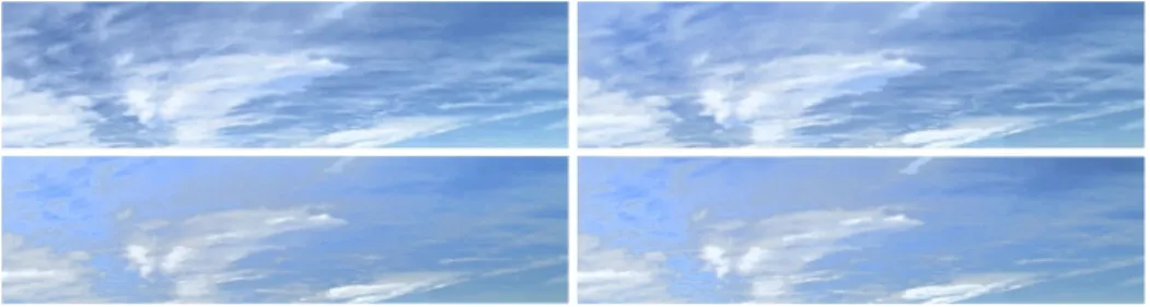
Figure 8. Sample outdoor images of the target data set derived from the AMOS data set [8].
Figure 9. The flowchart to measure the average normalized reconstructed error (ANRE). Some input blocks of the modules introduced in Figure 3 and 4 are not shown for clarity.
Table 1. The average ANRE of the target data set with both the uniform sky index model and our proposed model.
Sky Model Uniform Sky Index Model Our Model
Average ANRE 0.627 0.262
average changeDof two sky index images is measured by the following function:
D= n1n
i=1
|SIi1−SIi0|, (8) whereSIi1andSIi0are the sky indices of sky pixelsiwith the perturbed and original camera parameters respectively. Figure 10 shows the averageD of the target data set under variousΔθc andΔφc using the uniform sky index model (left half) and our model (right half). The sky index image of our model is more stable than that of the uniform sky index model under the perturbation ofθcandφc. The results are expected because when Δθc andΔφc achieve certain amounts, the uniform sky index model will force all pixels to take another sky index, but our model will only change the sky index of a pixelsiif theljmaximizingNCC(si, lj) changes.
5.3. Geo-location estimation
To compare the ability of predicting the longitude and latitude of the uniform sky index model and our model, we fixθc,φc, andf as the estimated values computed in Fig-ure 3 but hypothesize pairs of longitude and latitude (on a 5 degree grid). The estimated longitude and latitude is set to the hypothesis which maximizes Eq. (3). The flow of esti-mating the geo-location is shown in Figure 11 and executed with both the uniform sky index model and our model. We assume that we know the input image is taken from which hemisphere to increase the accuracy of geo-location
estima-Figure 10. The average change of sky index under different camera zenith and azimuth perturbations on the target data set. The aver-age change of our model (right half) is generally smoother than that of the uniform sky index model (left half).
tion. We search for the geo-location that maximizes the av-erage normalized cross correlation values between the sky maps and the input image at the corresponding location.
Accurate geo-location estimation often requires clear sky images [9, 12], shadow detection [21], or an image se-quence where the sun is visible [12]. Our model can pre-dict geo-location within 200 km in 4.55% of the target da-ta set given only single sky image. The 200 km thresh-old is inspired by [5]. The uniform sky index model only achieves the same criteria in 0.51% of the target data set. Figure 12 shows the portion of the prediction falling in d-ifferent thresholds of surface error. In general, the slope and the absolute value of the curve of our model are higher, which supports that our model has better geo-locating abil-ity. Further, our model predicts more accurate geo-location than the uniform sky index model in 66.67% of the images in the target data set. We also conduct a paired t-test to
com-Figure 11. The flowchart of estimating the geo-location based on the sky index.
Figure 12. The curves show the portion of the prediction falling in different thresholds of surface error, which supports that our model has better geo-locating ability.
pare the surface error made by both models for each image of the target data set;t(197) = 3.972,p = 0.0001. The average surface errors made by our model and the unifor-m sky index unifor-model are 4898 kunifor-m and 7209 kunifor-m respectively. Our data suggest that with 99.99% confidence, our model predicts more accurate geo-location than the uniform sky index model does.
6. Applications
In this section, we list several potential applications of our model, and sky image rendering is an obvious one. Giv-en the sky indices of all the sky pixels, we can rGiv-ender the corresponding sky images at any time and location by the flow in Figure 4. In other words, we can bring our favorite cloud distribution to the location and desired time that we want, which is impossible with the uniform sky index mod-el. Figure 13 demonstrates reconstructed images with the same cloud distribution under various times and locations. To colorize, the chromatic information in those images are kept the same as that of the input image without introducing another scattering model.
The sky indices derived from our model may serve as a source of features for cloud classification (cirrus, cumulus,
Figure 14. The estimation of cloud cover by our model. Each num-ber is the average sky index ranging from 0 (overcast) to 1 (clear) of the corresponding image.
stratus, etc.), providing important knowledge for weather forecasting as suggested in [3]. Tao et al. [18] estimate cloudiness of the sky and other semantic attributes to cat-egorize sky images, and we believe that it can achieve de-tailed classification by cloud types using our model. Fig-ure 14 orders the sky images based on the cloud cover by sorting the average sky indices. The sky indices of our mod-el are useful for cloud matching (deciding if two clouds are the same) or cloud tracking, a pre-processing step for some tasks in solar engineering [14].
Another potential application of our model is to achieve more accurate estimation of outdoor illumination condition-s condition-similar to the econdition-stimation in [11], and accurate illumina-tion models are needed for applicaillumina-tions such as shape from shading and artificial 3D object insertion in outdoor images. Note that in [11], sky is classified into one of the three cat-egories: clear, partially cloudy, or completely overcast ac-cording to the general sky appearance. The estimation of illumination conditions may benefit from our model incor-porating pixel-wise cloudiness prediction.
Figure 13. Reconstructed sky images with the same cloud distribution under various time and locations. The chromatic information in these images is kept the same as that of the input image without introducing another scattering model.
7. Conclusion
In this paper, we propose a novel sky representation that includes a pixel-wise sky index to represent clouds. We for-mulate our model as a labeling problem and solve the sky index for each sky pixel.
In our experiment, the proposed sky model surpasses the uniform sky index model in three ways: expressiveness, sta-bility under inaccurate camera parameter estimation, and the geo-locating ability. We also demonstrate using the sky index image to produce sky images with the given cloud distribution at desired time and location.
In the future, we will incorporate color information and model physical phenomena such as refraction and sunlight scattering improve the reconstructed sky images.
References
[1] Y. Boykov, O. Veksler, and R. Zabih. Fast approximate ener-gy minimization via graph cuts. IEEE Transactions on Pat-tern Analysis and Machine Intelligence, 23(11):1222–1239, 2001.
[2] A. P. Brunger and F. C. Hooper. Anisotropic sky radiance model based on narrow field of view measurements of short-wave radiance.Solar Energy, 51(1):53–64, 1993.
[3] R. Eastman and S. G. Warren. A 39-yr survey of cloud changes from land stations worldwide 1971–2009: long-term trends, relation to aerosols, and expansion of the tropi-cal belt.Journal of Climate, 26(4):1286–1303, 2013. [4] A. W. Harrison. Directional sky luminance versus cloud
cov-er and solar position.Solar Energy, 46(1):13–19, 1991. [5] J. Hays and A. A. Efros. IM2GPS: estimating geographic
information from a single image. InProceedings of the IEEE Conf. on Computer Vision and Pattern Recognition (CVPR), 2008.
[6] R. Hufnagel and M. Held. A survey of cloud lighting and rendering techniques. InProceedings of International Conf. on Computer Graphics, Visualization and Computer Vision (WSCG), 2012.
[7] N. Igawa, Y. Koga, T. Matsuzawa, and H. Nakamura. Models of sky radiance distribution and sky luminance distribution.
Solar Energy, 77(2):137–157, 2004.
[8] N. Jacobs, K. Miskell, and R. Pless. Webcam geo-localization using aggregate light levels. InWorkshop on Applications of Computer Vision (WACV), 2011.
[9] N. Jacobs, N. Roman, and R. Pless. Toward fully automatic geo-location and geo-orientation of static outdoor cameras. InWorkshop on Applications of Computer Vision (WACV), 2008.
[10] R. Kittler, R. Perez, and S. Darula. A new generation of sky standards. InProceedings of the Lux Europa, 1997. [11] J.-F. Lalonde, A. A. Efros, and S. G. Narasimhan. Estimating
the natural illumination conditions from a single outdoor im-age. International Journal of Computer Vision, 98(2):123– 145, 2012.
[12] J.-F. Lalonde, S. G. Narasimhan, and A. A. Efros. What do the sun and the sky tell us about the camera? International Journal of Computer Vision, 88(1):24–51, 2010.
[13] Q. Li, W. Lu, J. Yang, and J. Z. Wang. Thin cloud detection of all-sky images using markov random fields.IEEE Geosci. Remote Sensing Lett., 9(3):417–421, 2012.
[14] R. Marquez and C. F. M. Coimbra. Intra-hour dni forecast-ing based on cloud trackforecast-ing image analysis. Solar Energy, 91:327–336, 2013.
[15] R. Perez, R. Seals, and J. Michalsky. All-weather mod-el for sky luminance distribution–prmod-eliminary configuration and validation.Solar Energy, 50(3):235–245, 1993. [16] A. J. Preetham, P. Shirley, and B. Smits. A practical analytic
model for daylight. InProceedings of ACM SIGGRAPH, 1999.
[17] J. Schpok, J. Simons, D. S. Ebert, and C. Hansen. A real-time cloud modeling, rendering, and animation system. In
Proceedings of the ACM SIGGRAPH/Eurographics Sympo-sium on Computer Animation, 2003.
[18] L. Tao, L. Yuan, and J. Sun. Skyfinder: attribute-based sky image search. InProceedings of ACM SIGGRAPH, 2009. [19] The University of Arizona. (n.d.).The Arizona webcam.
Ari-zona webcam. Retrieved September 11, 2011, fromhttp: //www.cs.arizona.edu/camera/.
[20] C. J. Willmott and K. Matsuura. Advantages of the mean ab-solute error (MAE) over the root mean square error (RMSE) in assessing average model performance.Climate Research, 30:79–82, 2005.
[21] L. Wu and X. Cao. Geo-location estimation from two shad-ow trajectories. InProceedings of the IEEE Conf. on Com-puter Vision and Pattern Recognition (CVPR), 2010.
![Figure 1. An example of our proposed sky representation. The upper image is the input sky image (from [19])](https://thumb-us.123doks.com/thumbv2/123dok_us/1569940.2710794/1.918.478.825.350.563/figure-example-proposed-representation-upper-image-input-image.webp)
![Figure 8. Sample outdoor images of the target data set derived from the AMOS data set [8].](https://thumb-us.123doks.com/thumbv2/123dok_us/1569940.2710794/6.918.85.841.110.183/figure-sample-outdoor-images-target-data-derived-amos.webp)