Adaptive Query Execution for Data Management in the
Cloud
Adrian Daniel Popescu Debabrata Dash Verena Kantere Anastasia Ailamaki
School of Computer and Communication SciencesÉcole Polytechnique Fédérale de Lausanne CH-1015, Lausanne, Switzerland
{adrian.popescu, debabrata.dash, verena.kantere, anastasia.ailamaki}@epfl.ch
ABSTRACT
A major component of many cloud services is query process-ing on data stored in the underlyprocess-ing cloud cluster. The tradi-tional techniques for query processing on a cluster are those offered by parallel DBMS. These techniques, however, can-not guarantee high performance for cloud; parallel DBMS lack adequate fault tolerance mechanisms in order to deal with non-negligible software and hardware failures. MapRe-duce, on the other hand, allows query processing solutions that are fault tolerant, but imposes substantial overheads. In this paper, we propose an adaptive software architecture, which can effortlessly switch between MapReduce and par-allel DBMS in order to efficiently process queries regardless of their response times. Switching between the two archi-tectures is performed in a transparent manner based on an intuitive cost model, which computes the expected execution time in presence of failures. The experimental results show that the adaptive architecture achieves the lowest possible query execution time for various scenarios.
Categories and Subject Descriptors
H.2.4 [Database Management]: Systems
General Terms
Design, Performance
Keywords
Cloud DBMS, Cost Model, MapReduce, Parallel DBMS
1.
INTRODUCTION
Today we have an explosion of data collected from a wide range of applications. Traditional data warehouses have al-ready reached Peta-byte scale and are now being dwarfed by data collected in scientific applications [9, 20] or by the content generated online. For instance, eBay, a popular on-line auction and shopping website, uses 6.5 PB of data [10].
Permission to make digital or hard copies of all or part of this work for personal or classroom use is granted without fee provided that copies are not made or distributed for profit or commercial advantage and that copies bear this notice and the full citation on the first page. To copy otherwise, to republish, to post on servers or to redistribute to lists, requires prior specific permission and/or a fee.
CloudDB’10,October 30, 2010, Toronto, Ontario, Canada. Copyright 2010 ACM 978-1-4503-0380-4/10/10 ...$10.00.
Similarly Facebook, a social website, has reached 2.5PB of data, and growing at the rate of 15TB/day [11].
Running parallel DBMS on multiple hardware nodes is the traditional approach to address the above-mentioned chal-lenge. As early as the 1980s, several research prototypes such as Gamma [6] and Bubba [2], and several commercial products from Teradata [15] and Tandem [14] pioneered this approach. Parallel DBMS are highly optimized for per-formance and have been shown to scale up to one hundred nodes (e.g., eBay, the largest known database warehouse uses 96 nodes [10]). They, however, have several limitations. First, their fault tolerance mechanism is not adequate for the high failure rates on thousand node clusters based on com-modity hardware. Second, they enforce the relational data model, which can be too strict for modern data collections where 80% of the data is estimated to be unstructured or semi-structured [8].
As data continues to grow, new alternatives for data man-agement have emerged. Among them, MapReduce [5] and its open-source implementation Hadoop [16] have become popular. Unlike parallel DBMS, these systems scale to thou-sands of commodity nodes. MapReduce treats availability and fault tolerance as first class citizens with an architecture designed to resist multiple node failures, under-performing nodes, and hot spots. A growing number of enterprises scale their data analysis by using MapReduce. For example, Face-book uses Hadoop for managing its data warehouse [21, 22]. Parallel DBMS provide good performance and low latency, but do not scale to thousands of machines, and do not pro-vide elasticity. MapReduce on the other hand, provides scalability and elasticity, but has very high latency. It is desirable, therefore, to have a system that simultaneously provides scalability, elasticity, high performance and low la-tency.
Researchers proposed several such hybrid systems [1, 18], typically using MapReduce at the core of their technique to achieve the elasticity and scalability. We show that using MapReduce immediately adds overhead in the range of 10 to 20 seconds per query. While this is negligible for long-running queries which have response times of minutes or more, it significantly reduces the performance for the faster queries which need be answered within seconds.
A representative hybrid system is HadoopDB [1], which targets query performance comparable to parallel DBMS, and the fault tolerance and scalability of MapReduce. The main idea is to deploy a traditional DBMS across all the processing nodes and use MapReduce as the communication layer between them. HadoopDB achieves high performance
by pushing a large fraction of work into the DBMS layer and achieves fault tolerance by using MapReduce to parallelize query computation across DBMS nodes. HadoopDB is un-suitable for short-running queries for several reasons. First, HadoopDB uses MapReduce as its communication layer in-dependent of how much query work is pushed into the DBMS layer. Therefore, HadoopDB always pays the MapReduce overhead. As shown in Section 2, this overhead becomes significant for short-running queries. Second, HadoopDB ar-chitecture uses traditional DBMS that usually do not match the fault tolerance and elasticity properties of today’s cloud storage engines. Specifically, the lack of elasticity does not allow the DBMS to adapt to addition or removal of process-ing nodes – a common operation for any cloud system.
In this paper, we propose a hybrid approach that per-forms well for both short-running and long-running queries. We achieve this by building a cost model on top of a parallel DBMS and MapReduce to determine the best possible exe-cution model for a given query. We also leverage a scalable and elastic storage engine–HBase [17], in order to provide the desired elasticity at all levels of the framework. HBase is also more suitable for the semi-structured data than the relational DBMS.
Compared to the state of the art hybrid approaches, our proposed solution makes the following contributions:
• An architecture for a cloud DBMS, all components of
which are fault-tolerant, scalable, and elastic.
• An adaptive scheme capable of deciding where to
exe-cute a query based on its estimated running time, the number of processing nodes and the failure rate of the processing nodes.
• A set of representative experiments showing the
bene-fits of the adaptive scheme for a range of queries. The rest of the paper is organized as follows. Section 2 introduces the background and the motivation for our work. Section 3 presents the software architecture. Section 4 in-troduces our proposed adaptive scheme. Section 5 presents the experimental setup. Section 6 presents a set of repre-sentative results. Section 7 continues with related work and finally, Section 8 concludes.
2.
BACKGROUND AND MOTIVATION
In this section, we discuss (at a high-level) parallel DBMS, then MapReduce, and finally illustrate with an example the overhead of the MapReduce tasks for short-running queries. In the rest of the paper we define a query as a “long-running query” if its execution time is comparable to or higher than the overhead of MapReduce. A query with lower execution time is defined as a “short-running query”.
2.1
Parallel DBMS
The subject of extensive research in the 80s; parallel DBMS execute queries by dividing the work and running concur-rently on multiple processing nodes. Among several pro-posal towards designing the architecture of parallel DBMS, shared-nothing has been the most successful [12] as shown in the Bubba and Gamma parallel architectures. In this execu-tion model, the data is partiexecu-tioned across several data nodes. A scheduler receives the query which is further scheduled
for execution on the nodes containing the data. If the query touches multiple data nodes, then the data is transferred across the network to the appropriate processing nodes.
Since fault tolerance was not that important during the development of these systems, the data is always streamed across different nodes and operators in the query. The stream-ing implies that, in case a node fails, the query has to be restarted from the very beginning. When failures become more frequent, this can lead to very low query throughput and very high response times.
2.2
MapReduce
MapReduce follows the shared-nothing approach, but with several key differences from the parallel DBMS approach. Firstly, the data is partitioned across the nodes, however, a file system is designed to provide a unified view of the data [7]. Moreover, the data is replicated several times to ensure reliability and locality on the processing nodes which need it. This implementation of the filesystem keeps the popular nothing architecture but provides a shared-disk view to the client of the data.
A query in MapReduce is split into two types of tasks: map tasks and reduce tasks. The map tasks process one relation at a time and transform the input data (e.g., fil-ter, project); the reduce tasks collect the output data from the map tasks to do further processing such as join or ag-gregation. There can be several stages of such map and reduce tasks to process complex queries. Several systems that translate SQL queries into such map and reduce tasks automatically were introduced [3, 18, 19]. The crucial differ-ence between MapReduce and parallel DBMS is that each time part of the computation is done by the map or the reduce tasks they are checkpointed on the disk. In case of processing node failure, the computation can be restarted by collecting the saved results from the disk and restarting the pending tasks. The on-disk checkpoints allow MapReduce to handle node failures well, at the expense of performance. Furthermore, MapReduce-based systems have been focus-ing on the large batch oriented queries runnfocus-ing from hours to days, ignoring the queries taking milliseconds to tens of seconds.
2.3
Need for a Hybrid Approach
In this paper we argue that a cloud DBMS should run long-running queries efficiently, while not sacrificing the per-formance of the short-running queries. The long-running queries are required to run large-scale data analysis. The short-running queries are required to enable interactive anal-ysis of the data, and provide real-time feedback. We now discuss a use case for both types of queries.
Many astronomers use the data repository provided by the SDSS skyserver [13] to conduct their research. The data is stored in locations around the world, and thousands of astronomers access them. Although the data size is large (7 TB), each astronomer typically focuses on a small cor-ner of the sky and poses queries, which are executed within 2 seconds on average [24]. Significantly slowing down such short-running queries would affect the research negatively, as they are mostly interactive exploratory queries. The as-tronomers also pose large queries, which take hours to com-plete, for example when they validate the models over large patches of the sky. Therefore, if the service were to be moved
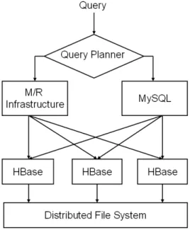
Figure 1: The software architecture of the hybrid approach. Based on the query type, the number of processing nodes and the failure rate of the process-ing nodes, HBaseSQL or MapReduce is chosen to execute the query.
to a cloud, it has to answer both the short-running and the long-running queries efficiently.
Neither MapReduce nor parallel DBMS provide the best solution for both types of queries. MapReduce provides bet-ter fault tolerance, scalability and elasticity, while parallel DBMS provides better performance. Long-running queries are executed more efficiently using MapReduce due to their higher probability of failure. On the other hand, short-running queries have much lower probability to fail; there-fore, they are executed more efficiently using parallel DBMS. Therefore, we seek to develop a hybrid system capable of si-multaneously exploiting the benefits of both.
As an example, we use a point select query that runs on top of an index table with 1.5 million rows with a very low selectivity (1 out of 1.5 million). Only one map task is used for this query which does not output any intermediate results and hence the reduce task is avoided. The complete exper-imental setup and methodology can be found in Section 5. MapReduce approach takes about 21 seconds to complete this query.
The time breakdown for MapReduce is as follows: the scheduling overhead (3 seconds), the overhead of running the map task (12 seconds), and the actual work – a filtered scan operation (6 seconds). In total, MapReduce has a 15 second overhead which is significant compared to the ac-tual filtered scan operation. Therefore, we argue that short queries should be executed outside MapReduce; since they run in a short amount of time, the effect of node failure is not as important as for long running queries.
3.
SYSTEM ARCHITECTURE
The system architecture is designed to satisfy both short-running and long-short-running queries efficiently. When a query
enters into the system, the query planner decides where to execute it, i.e. in parallel DBMS or in MapReduce. A key characteristic of the system is that the same storage layer is used for both query execution models. This design choice reduces the overhead of managing the data twice. Figure 1 shows the high-level architecture. In what follows, we ex-plain each software component in detail.
Distributed File System: Our software infrastructure is deployed on a cluster where each machine acts both as a storage and as a processing node. Even though we adopt a shared nothing architecture, where each machine has its own memory, disk and processing resources, we develop our system on top of a distributed file system [7] which is opti-mized for fault tolerance, availability, and elasticity. We use Hadoop Distributed File System (HDFS), an open source implementation included in the Hadoop software distribu-tion. The data is partitioned and replicated across several nodes in the system, allowing easy node additions or re-movals. Additionally, the distributed file system presents a simple interface to applications, removing the burden of replicating data at the higher layers in the software stack.
HBase: HBase is the storage manager component in charge of managing the data. HBase allows the execution of basic CRUD (Create, Read, Update, Delete) operations, but it does not support the execution of complex query operators (e.g., joins, aggregations) common in analytical applications. Therefore, a query execution layer is needed above the stor-age layer.
HBase has several advantages over traditional storage sys-tems. Firstly, HBase supports both structured and semi-structured data through a flexible data layout that relaxes the schema constraints from the traditional row stores. Sec-ondly, HBase trades-off strong consistency guarantees for weaker consistency models that allow for better availability. In analytical workloads where most of the queries are reads, paying the additional cost for ensuring strong consistency is not justified. Thirdly, HBase is built on top of Hadoop’s Distributed File System; thus, it shares the same level of fault tolerance and elasticity as Hadoop.
To achieve scalability on the input data, HBase partitions relations based on a row key. Each partition (or region) is assigned to a server node in the cluster, called the re-gion server. A master node coordinates rere-gion allocations to region servers based on data locality, and also performs relocation of regions in the case a region server fails. When a query requires data from a particular region, the client queries the master node for the region location, and directly contacts the region server to access the data.
MapReduce: MapReduce is one of the software compo-nents that we use to parallelize query execution. Running MapReduce tasks on top of a semi-structured storage engine such as HBase ensures better query performance than the “raw” MapReduce. Using HBase avoids the parsing over-head of “raw” MapReduce. Furthermore, query operators (such as scans or filters) and query optimization techniques (such as indexes) are available in HBase. MapReduce en-sures fault tolerance and load balancing across the process-ing nodes, but as presented in Section 2, it reduces perfor-mance for short-running queries due to the overheads in-duced by its scalable infrastructure. For running complex
analytical queries using MapReduce, we use Hive [18] to translate the input SQL query into the optimal query plan expressed as a set of MapReduce jobs.
MySQL: MySQL is the execution engine used to paral-lelize query execution for the short-running queries. When a query is sent to MySQL execution engine, the engine pro-cesses the query as follows. First, it determines the location of all the HBase region servers that hold the input relation. Then, it distributes parts of the query computation (i.e., scans, filters operators) to the HBase region servers that hold the data. Finally, it collects the data from the HBase region servers on a master node and executes the complex query operators inside the MySQL execution engine.
The combination of MySQL execution engine with HBase storage, in shortHBaseSQL, has several advantages. First, it uses a traditional DBMS execution engine that does not have the same overhead as MapReduce. Second, it has the potential of improving the query performance by employing a dedicated query optimizer for choosing the best query plan. Finally, it offers more usability to the user who otherwise would need to implement complex query operators at the application layer.
We design and implement HBaseSQL as a plug-in that can be loaded at run-time inside MySQL server in a similar manner to other storage engines (e.g., MyISAM, InnoDB). Requests to HBaseSQL are triggered directly by MySQL server when the user queries a table that defines HBaseSQL as its storage engine. HBaseSQL communicates with HBase through a connector interface that allows calling HBase na-tive code (Java) from C++. For this purpose, we use the JNI interface. JNI allows Java code that runs inside a Java Virtual Machine to call or to be called by other languages, such as C or C++.
Query Planner: The last component of our system is the query planner, which takes the decision on where to execute the query: HBaseSQL or MapReduce. This decision is taken based on a cost model that uses query characteristics and the node failure rate to compute the estimated cost of the query in the presence of failures. Then, the approach with the lower estimated cost is chosen to execute the query; details of the cost model are described in the next section.
4.
ADAPTIVE QUERY EXECUTION
Since MapReduce performs better than HBaseSQL under failure, the choice of using either of these frameworks de-pends on the query failure probability. The query failure probability depends on the following factors: failure rateof the individual processing nodes, thetotal work required by the query, and thenumber of nodeswhich process the query. As all of these parameters affect the query failure probabil-ity, none of them considered in isolation can provide the best decision regarding what query execution engine to use. Therefore, we introduce a cost model which estimates the expected cost of the query in the presence of failure for both frameworks. This cost model enables direct comparison of the efficiency of the two approaches and allows us to com-pare them directly.
Intuitively, short running queries that are processed on a small set of nodes have a low probability of failure. Thus, processing the query in HBaseSQL is more efficient, as it avoids the overhead of the fault tolerance mechanism in
MapReduce. On the other hand, long-running queries that run for several hours to complete their execution and that use hundreds to thousands of nodes have a high probability of failure. Therefore, they are executed as MapReduce jobs which have the advantage of dividing the query work into several sub-tasks that checkpoint their intermediate results on disk. Hence, a complete query restart is avoided in the case the query fails. This allows MapReduce to finish the query execution faster than traditional database approaches which always re-start the query in the case one of the pro-cessing nodes fails.
4.1
Cost Model
Upon receiving a query, the planner computes its expected cost in the following two cases: first, when the query is ex-ecuted in HBaseSQL layer and, second, when the query is executed on top of MapReduce. The infrastructure provid-ing the lowest execution cost runs the query.
4.1.1
Query Execution in HBaseSQL
We assume the following execution model for the query in HBaseSQL. The optimizer receives the queryq, and dis-tributes the computation among n HBase nodes. Data is then collected from the HBase nodes on a master node which runs the join and aggregation to answer the query. Let
tqi, i= 1, ..., nbe the time taken by each of the HBase nodes,
OHB be the scheduling time taken by the master node to
distribute the computation among the HBase nodes. Since the scheduling overhead depends on the failure rate, and the number of nodes,oHBis a function of these two factors. Let
tqmbe the time taken by the master node doing the join and
aggregation operations.
The total time to run the query is:
tq=tqm+oHB(f, n) +
n
max
i=1 tqi
And the total work done to answer the query is:
wq=tqm+oHB(f, n) +
n
X
i=1
tqi
Since the HBaseSQL implementation is straightforward, we incur very low overhead for scheduling the queries. There-fore, we assume that oHB(f, n) = 0. We also assume that
the nodes in the cluster are homogeneous, and have the same rate of failuref per unit time. We considerf to be the ag-gregated failure rate of all the hardware and software com-ponents of a node used in the query execution. As for the model of running queries on HBaseSQL, if any of the nodes fail, then the entire query needs to be re-executed.
Therefore, the probability of restarting the query:
fq= 1−(1−f)wq (1)
The expected cost of running the queryq on the DBMS becomes: CostHB(q, f) = ∞ X i=1 wq×fqi−1= wq 1−fq = wq (1−f)wq (2)
The intuition behind the equation is as follows. If the query does not fail then we pay the cost wq. If however it
fails, which is a function of probabilityfq, then we pay the
costwq again. This continues until the query executes to
completion.
4.1.2
Query Execution in MapReduce
The MapReduce scheduler receives the query and splits it intommap tasks andrreduce tasks. If any of these tasks fails, then only the failed task is re-executed. The reduce tasks wait for the map tasks to complete before starting the processing. Once more, we assume the cluster is homoge-neous, with a node failing rate off per unit of time.
Lettmj be the cost of running thejthmap task, andtrk
be the cost of running the kth reduce task. As shown in
Section 2, the MapReduce jobs also carry some overhead, and we denote the overhead as OM R. In absence of any
failures, the total cost of running the MapReduce job is:
OM R+ m X j=1 tmj+ r X k=1 trk
In the presence of failures, the map and the reduce tasks should be restarted. Using the failure ratef, and equations similar to the cost for running the query in the DBMS, the cost becomes: CostM R(q, f) =oM R(f, m, r) + m X j=1 tmj (1−f)tmj + r X k=1 trk (1−f)trk (3) The first term,oM R(f, m, r), is the overhead of the
MapRe-duce job as a function of the failure ratef, the number of map tasksm, and the number of reduce tasksr. In our em-pirical model we approximateoM R(f, m, r) with OM R, the
job overhead in the absence of failures, as the best case for the MapReduce approach. We are currently investigating a more accurate definition for the MapReduce overhead when failures occur.
4.2
Examples
In what follows, we give two examples to show the advan-tages of each of the above two approaches.
Example 1: Let us assume a query that runs on 1000 ma-chines and performs an aggregation on a selected attribute. Further, consider that the query’s work is uniformly split across all the machines and thattqi= 10 minutes,tqm= 10
minutes. Therefore, the total work done to answer the query is wq=167 machine-hours. Let f be 0.0007 per minute,
which corresponds to the failure rate of a MapReduce job as reported in [5]. According to Equation 1, the probabil-ity that the query fails during its execution in HBaseSQL is 99.90%. Using Equation 2, we obtain the estimated cost of the query to be about 21 machine-years. This result shows the query will never finish if it is executed in HbaseSQL.
Similarly, we compute the cost of the query for MapRe-duce. In this case, we assume m = 1000 andr = 1. Fi-nally, we assume thattmj=11 minutes and thattrk=11
min-utes, which includes a checkpointing cost of 1 minute. The MapReduce overhead OM R is in the order of seconds and
hence negligible for this example. The map tasks scan the input table and generate intermediate aggregation results, while the reduce task merges the intermediate results pro-ducing the final result. Using Equation 3, the total cost of running the query in MapReduce is 185 machine-hours. We
clearly observe that MapReduce incurs a much lower cost than HBaseSQL in this example.
Example 2: In this example, we consider a shorter query that runs only on 100 machines and that tqi = 1 minute,
tqm = 1 minute leading to a total work time for answering
the query of wq = 101 machine-minutes. For HBaseSQL,
the probability that the query fails is 6%, therefore, the overall cost for running the query is estimated to be 108 machine-minutes. Conversely, using MapReduce with the same checkpointing cost of 1 minute as in Example 1, we havetmj=2 minutes,trk=2 minutes. As a result we obtain
an overall cost of 202 machine-minutes. In this case, the expected cost of executing the query in MapReduce is higher than the cost in HBaseSQL. Therefore, our adaptive scheme chooses to execute the query in HBaseSQL.
4.3
Discussion
In order to make the decision about which framework to run the query, the planner requires query statistics (such as
tqi, tqm, tmj, trk, OHB, OM R) and the failure rate of the
processing nodes (f). We assume that all these parameters can be determined using a statistics module built on top of MySQL’s optimizer. Additionally, the statistics module can be extended with a feedback-loop mechanism capable of adjusting the query parameters based on recently measured values. For failure rates, we consider them constant and that all the machines are homogeneous having the same failure rates. Even for cases when the nodes have heterogeneous failure rates, we can easily adjust our formulas to take them into consideration. We are currently working on the design and implementation of such a statistics module.
5.
EXPERIMENTAL SETUP
Software Configuration: We use Hadoop version 0.20.2 and HBase version 0.20.3. We allocate 1GB of memory for Hadoop and 4GB of memory for HBase out of which 1.6 GB is allocated for caching the data. We use MySQL version 9.5.1 to build HBaseSQL, and use Hive query engine to ex-ecute queries on MapReduce. Hive also uses the underlying HBase storage engine, instead of using a separate storage.
Hardware Configuration: We use 5 hardware machines, each of which is an X4140 Sun Machine with 2 quad CPUs AMD Opteron 64-bit @ 2700 MHz, 32 GB RAM, 1 Gb net-work connection, 8 SAS disk drives at 10,000 RPM with 1.2 TB of data allocated for the Hadoop File System. The OS that we use is Linux Ubuntu 9.04.
Methodology: We use two different methodologies to perform our evaluation. Firstly, we validate our adaptive query execution scheme by generating failures in the sys-tem and measuring the query execution cost for the two approaches: MapReduce and HBaseSQL. Secondly, we eval-uate the performance benefits of HBaseSQL for running queries in the cloud.
Data Set: In our experiments we use the orders and
lineitem tables from the TPCH benchmark [23]. Unless
otherwise stated, we load a lineitem data file of 6 million rows and an orders data file of 1.5 million rows in HBase. Each row has an approximate size of 100 bytes. The data is stored in HBase using a row store data layout. This data layout translates to a storage size of 6 GB for lineitem table and 900 MB for orders table. To speed up the joins we
No of rows wq[s] tq[s] tm[s] OM R[s] 5 0.1 0.02 3 14 1 mil. 37 7 12 11 3.5 mil. 124 24 33 12 15 mil. 678 136 137 12 30 mil. 1466 293 310 12
Table 2: Measured query parameters required in validating our adaptive query execution scheme.
Machine M1 M2 M3 M4 M5
Failing Time Interval [min] 16 3 - 7 10
Table 3: A failure distribution instance correspond-ing to a failcorrespond-ing rate of f = 1/30min (1 failure in 30 minutes).
build indexes onl orderkey, and ono orderkeyfields of the
lineitemandorderstables respectively.
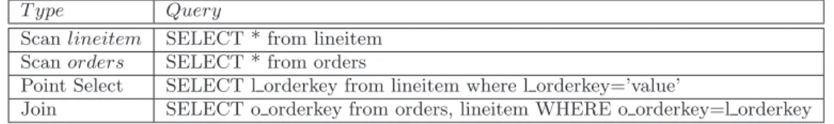
Benchmarks: We use synthetic benchmarks to evaluate the performance of our adaptive approach. We evaluate the performance of queries containing table scans, point selects, and joins. Table 1 shows the list of queries that we use in our experiments.
Metrics: For the purpose of this evaluation we use re-sponse time and query cost as our metrics of interest. The latency is the actual query execution time, while the query cost is the aggregated query work performed by each node processing the query, as defined in Section 4.
Running Experiments: Our data set can fit in the memory easily. Hence, in the case of each of the experiments we start with cleaned OS caches. Moreover, we also clean the MySQL and HBase caches by killing and re-starting them before each experiment. Each experiment is run at least five times and we report the averages.
6.
EVALUATION
In this section we present a set of experiments that show the benefits of our adaptive query execution scheme for a variety of queries. First, the analytical formulas introduced in Section 4 are validated, then a set of experiments demon-strates the benefits of using HBaseSQL.
6.1
Adaptive Query Execution Scheme
To verify our formulas from Section 4, we use a scan query on theorderstable for several input table sizes. As we consider a simple selection operation that reads the in-put table without storing or generating any result on disk, the corresponding MapReduce job does not require a reduce job. Therefore, the relative performance difference between MapReduce and HBaseSQL is the best possible for MapRe-duce. In our experiments, we do not use a statistics module. Therefore, we obtain the query parameters provided in Sec-tion 4 by sampling real execuSec-tions of the queries when no failures occur. Table 2 shows all these parameters for a fail-ure rate off= 1/30min(1 failure in 30 minutes). As the selection query does not perform any additional work, we havetqm= 0 andtr= 0.
We use a failure rate of f = 1/30 min, in proportion to our small cluster setup. We use a uniform distribution
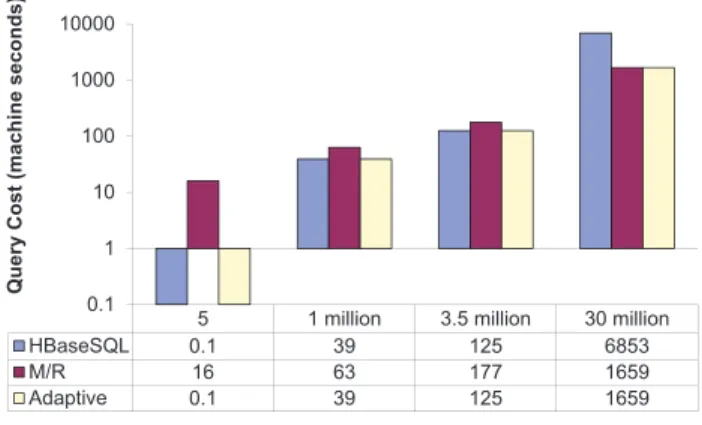
5 1 million 3.5 million 30 million HBaseSQL 0.1 39 125 6853 M/R 16 63 177 1659 Adaptive 0.1 39 125 1659 0.1 1 10 100 1000 10000 Q u e ry C o s t (m a c h in e s e c o n d s ) Number of rows
Figure 2: Query execution cost as a function of input table sizes.
1/3 min 1/5 min 1/10 min 1/20 min No failure HBaseSQL 11017 5317 817 667 667 M/R 1130 867 782 696 696 Adaptive 1130 867 782 696 667 1 10 100 1000 10000 Q u e ry C o s t (m a c h in e s e c o n d s ) Failure Rate
Figure 3: Query execution cost as a function of nodes failure rate.
for generating the time points of failure corresponding to the failure ratef by dividing the lifespan of a machine into several discrete intervals of one minute each and associating to each interval a uniform probability of failure. Table 3 shows an instance for the failure distribution justifying the decisions taken by our adaptive query execution scheme.
Figure 2 illustrates the actual query execution cost for four different input table sizes. Our algorithm selects HBaseSQL for short running queries because the aggregated failure rate is low enough to keep the query cost below the corresponding cost of MapReduce. For longer running queries (e.g., the one that reads 30 million rows) our algorithm chooses to use MapReduce because the duration of the query approaches the machine failure interval, thus increasing the probability of failure (according to Equation 1). MapReduce is efficient in this case, having a total query cost of more than four times lower than the corresponding cost in HBaseSQL; this can be explained by observing the query in HBaseSQL fails three times in a row, and is followed each time by a complete query restart.
T ype Query
Scanlineitem SELECT * from lineitem
Scanorders SELECT * from orders
Point Select SELECT l orderkey from lineitem where l orderkey=’value’
Join SELECT o orderkey from orders, lineitem WHERE o orderkey=l orderkey
Table 1: Micro-benchmark queries used for evaluating HBaseSQL with MapReduce.
To validate our formulas on several different failure rate parameters, in the following experiment we keep the input table size constant and we vary the failure rate parameter. We fix the table input size to 15 million rows and we vary the failure rate between 1 in 3 minutes to 1 in 20 minutes. The corresponding query parameters are presented in Table 2. As with the previous experiment, we use a uniform fail-ure distribution to obtain the time points of failfail-ure for each hardware machine.
Figure 3 shows the measured query execution costs. As ex-pected, at high failure rates, running the query in HBaseSQL is expensive as it resorts to re-starting it over and over again until eventually completes. This is exactly what happens for
f= 1/3min andf= 1/5min(1 failure in 3 minutes, and 5 minutes respectively), where the query is re-started 7 and 5 times, respectively. As the failure rate decreases, the dif-ference in performance reduces. Atf = 1/10minwe have only one query restart and atf= 1/20minthe query does not fail at all. We observe that for all cases our adaptive al-gorithm chooses to run the query using MapReduce due to the fact that the estimated query cost (of about 2 minutes) combined with the number of machines on which the query executes (i.e., 5) contributes to a high aggregated failure rate.
Since our algorithm is probabilistic in nature, it can make mistakes. Specifically, it can make wrong choices when the aggregated failure rate interval is relatively close to the query running time, but failures do not occur during this inter-val. We can notice such a point for the failure rate of
f = 1/20 min. But the difference in the query execution time for MapReduce and HBaseSQL is low in such cases; therefore, the error in the model does not affect the perfor-mance of the queries.
6.2
Comparing HBaseSQL Performance with
MapReduce
In this set of experiments, we evaluate the performance of scan, point select, and join operations for HBaseSQL and MapReduce, in absence of any failures. Table 4 shows the execution times for the queries defined earlier.
Scan: In terms of scan operations, the performance of HBaseSQL is 20% better than MapReduce. This result is encouraging for us showing that the overheads of HBaseSQL are lower than that of the established MapReduce implemen-tation in Hive.
Point Select: For point select queries HBaseSQL per-forms much better than MapReduce. Hive’s MapReduce implementation performs poorly, as it does not exploit the indexes. Hence, whenever selecting a single row for a par-ticular column value, a full table scan operation is required.
Join: Finally, in the case of the join query,orders and
lineitemtables are joined on theo orderkeyandl orderkey
attributes, respectively. Since these columns are already
in-Query type HBaseSQL[s] MapReduce[s]
Scan 1056 1270
Point Select 0.9 440
Join 1753 598
Table 4: Micro-Benchmark results for HBaseSQL for scan, point select and join operations.
dexed, the main table is never touched. The results show that HBaseSQL performs about 3 times worse than MapRe-duce due to the use of two different joining algorithms for MySQL (nested-loops), and Hive (sort-merge). MySQL ex-ecution engine uses nested-loops as the default join algo-rithm for tables that are indexed on the matching field and block-nested loops otherwise. In this case,lineitemtable is indexed onl orderkeyattribute, therefore the nested-loops algorithm is chosen. Hive, on the other hand, uses a repar-titioning sort-merge algorithm that proves to be more ef-ficient than the nested-loop algorithm. Currently we are implementing better joining algorithms for HBaseSQL.
7.
RELATED WORK
MapReduce [6] have been introduced to scale indexing operations. Although it generated a lot of interest among many users, MapReduce has its own drawbacks that make its adoption as a simple replacement for traditional parallel DBMS disputable. The work of Pavlo et al. [5] argues in favor of traditional parallel DBMS and shows MapReduce is more expensive for complex query operators because not all of the query operators can be efficiently translated into the MapReduce programming model. In our approach, query execution is performed either entirely inside the database layer or on top of MapReduce, depending on the input query type and the failure rate of the processing nodes.
A precursor of HadoopDB [1], Hive [18] is a hybrid ap-proach that allows for the execution of SQL queries on top of the MapReduce infrastructure. Hive stores relations as files inside a distributed file system and automatically trans-lates HiveQL queries, a variant of SQL, into MapReduce jobs. The produced MapReduce jobs are further processed traditionally on top of the MapReduce infrastructure. In addition to similar approaches that translate SQL queries into MapReduce jobs [3, 19], Hive adopts a query optimizer that selects the most efficient query plans. A disadvantage of Hive is that it always executes SQL queries as MapRe-duce jobs. As already explained, MapReMapRe-duce is inefficient for short queries that should execute rapidly.
The work of Condie et al. [4] introduces MapReduce On-line, a modified MapReduce architecture that achieves bet-ter performance for MapReduce jobs by pipelining data across Map/Reduce tasks rather than materializing them on disk.
This optimization enables MapReduce to work for online queries, but it does not affect the MapReduce scheduling overheads.
The work of Yang et al. [25] introduces Osprey, a system which implements MapReduce-style fault tolerance for a dis-tributed DBMS. In Osprey, each query is split into several subqueries, which are executed on different processing nodes such that if a node fails the amount of work lost is at most one subquery’s work. Therefore, failing queries do not have to be restarted from the ground up. As compared with our work, Osprey is not designed to optimize performance for short running queries, which needlessly pay the additional cost of check-pointing.
8.
CONCLUSIONS
In this paper we motivate the case for “short-running” queries that suffer performance on popular data analysis techniques such as MapReduce. In order to process both short-running queries and long-running queries efficiently, we introduce an adaptive query execution scheme that makes the scheduling decision either for MapReduce or for parallel DBMS based on a cost model. The model takes as the input the query and the probability of node failures and outputs the decision on where to execute the query. We have seen that MapReduce is preferred for long-running queries that have a higher probability to fail. Conversely, parallel DBMS is more efficient for short-running queries as it removes the scheduling and checkpointing overheads of MapReduce. Our experiments show that the adaptive scheme provides two orders of magnitude speedup compared to MapReduce for short-running queries, while it preserves the advantages of MapReduce for long-running queries.
Acknowledgments
The authors would like to thank the anonymous reviewers for their comments and suggestions. We would also like to thank Thomas Heinis, Ryan Johnson and Daniel Lupei for their insightful feedback and suggestions which contributed significantly to the improvement of this work.
9.
REFERENCES
[1] A. Abouzeid, K. Bajda-Pawlikowski, D. Abadi, A. Silberschatz, and A. Rasin. HadoopDB: an architectural hybrid of MapReduce and DBMS technologies for analytical workloads.Proc. VLDB Endow., 2(1):922–933, 2009.
[2] H. Boral, W. Alexander, L. Clay, G. Copeland, S. Danforth, M. Franklin, B. Hart, M. Smith, and P. Valduriez. Prototyping Bubba, a highly parallel database system.TKDE, 2(1):4–24, 1990.
[3] Concurrent Inc. Cascading Project Website: http://www.cascading.org/.
[4] T. Condie, N. Conway, P. Alvaro, J. M. Hellerstein, K. Elmeleegy, and R. Sears. MapReduce online. Technical Report UCB/EECS-2009-136, EECS Department, University of California, Berkeley, 2009. [5] J. Dean and S. Ghemawat. MapReduce: simplified
data processing on large clusters. InOSDI, 2004. [6] D. J. DeWitt, S. Ghandeharizadeh, D. A. Schneider,
A. Bricker, H. I. Hsiao, and R. Rasmussen. The Gamma database machine project.TKDE, 2(1):44–62, 1990.
[7] S. Ghemawat, H. Gobioff, and S.-T. Leung. The Google file system.SIGOPS Oper. Syst. Rev., 37(5):29–43, 2003.
[8] R. Gilbert and R. Winter. Scale for success: will new requirements max out your data warehouse ? Scaling Up, WinterCorp, Newsletter Website:
http://www.wintercorp.com/Newsletter/wcnl spring06 e.pdf, 2006.
[9] MICS Project. MICS Project Website: http://www.mics.org/.
[10] C. Monash. eBay’s two enormous data warehouses. DBMS2 - A Monash Research Publication. http://www.dbms2.com/2009/04/30/ebays-two-enormous-data-warehouses.
[11] C. Monash. Facebook, Hadoop, and Hive. DBMS2 - A Monash Research Publication.
http://www.dbms2.com/2009/05/11/facebook-hadoop-and-hive.
[12] M. Stonebraker. The case for shared nothing.IEEE Database Eng. Bull., 9(1):4–9, 1986.
[13] A. S. Szalay, J. Gray, A. R. Thakar, P. Z. Kunszt, T. Malik, J. Raddick, C. Stoughton, and
J. vandenBerg. The SDSS skyserver: public access to the sloan digital sky server data. InSIGMOD, 2002. [14] Tandem Database Group. NonStop SQL: A
distributed, high-performance, high-availability implementation of sql. InHPTS, 1989.
[15] Teradata Database. Teradata Website: http://www.teradata.com.
[16] The Apache Hadoop Framework. Hadoop Project Website: http://hadoop.apache.org.
[17] The Apache Hadoop HBase Project. HBase Project Website: http://hadoop.apache.org/hbase/. [18] The Apache Hive Project. Hive Project Website:
http://hadoop.apache.org/hive/.
[19] The Apache Pig Project. Apache Pig Project Website: http://hadoop.apache.org/pig/.
[20] The Brain Blue Project. Brain Blue Project Website: http://bluebrain.epfl.ch/.
[21] A. Thusoo, J. S. Sarma, N. Jain, Z. Shao, P. Chakka, N. Zhang, S. Antony, H. Liu, and R. Murth. Hive: A petabyte scale data warehouse using Hadoop. In ICDE, 2010.
[22] A. Thusoo, Z. Shao, S. Anthony, D. Borthakur, N. Jain, J. Sen Sarma, R. Murthy, and H. Liu. Data warehousing and analytics infrastructure at Facebook. InSIGMOD, 2010.
[23] Transaction Processing Performance Council. TPC-H Website: http://www.tpc.org/tpch/.
[24] X. Wang, T. Malik, R. Burns, S. Papadomanolakis, and A. Ailamaki. A workload-driven unit of cache replacement for mid-tier database caching. In DASFAA, 2007.
[25] C. Yang, C. Yen, C. Tan, and S. Madden. Osprey: Implementing MapReduce-style fault tolerance in a shared-nothing distributed database. InICDE, 2010.