Subdivision for Modeling and Animation

(1)

SIGGRAPH 99 Course Notes

Subdivision for Modeling and Animation

Organizers: Denis Zorin, New York University

(2)

(3)

Lecturers

Denis Zorin

Media Research Laboratory

719 Broadway,rm. 1201

New York University

New York, NY 10012

net:

[email protected]

Peter Schr¨oder

Caltech Multi-Res Modeling Group

Computer Science Department 256-80

California Institute of Technology

Pasadena, CA 91125

net:

[email protected]

Tony DeRose

Studio Tools Group

Pixar Animation Studios

1001 West Cutting Blvd.

Richmond, CA 94804

net:

[email protected]

Jos Stam

Member Technical Staff

Alias

j

wavefront

1218 First Avenue, 8th Floor

Seattle, WA 98104

net:

[email protected]

Leif Kobbelt

Computer Graphics Group

Max-Planck-Institute for Computer Sciences

Im Stadtwald

66123 Saarbr¨ucken, Germany

net:

[email protected]

Joe Warren

Computer Graphics and Geometric Design Group

Computer Science Department

Rice University

Houston, Tx 77584

(4)

(5)

Schedule

Morning Session: Introductory Material

The morning section will focus on the foundations of

sub-division, starting with subdivision curves and moving on to surfaces. We will review and compare a

number of different schemes and discuss the relation between subdivision and splines. The emphasis

will be on properties of subdivsion most relevant for applications.

Foundations I: Basic Ideas

Peter Schr¨oder and Denis Zorin

Foundations II: Evaluation and survey of subdivision schemes

Denis Zorin and Jos Stam

Afternoon Session: Applications and Algorithms

The afternoon session will focus on applications

of subdivision and the algorithmic issues practitioners need to address to build efficient, well behaving

systems for modeling and animation with subdivision surfaces.

Implementing Subdivision and Multiresolution Meshes

Denis Zorin

A Variational Approach to Subdivision

Leif Kobbelt

Variational Subdivision Cookbook

Joe Warren

Subdivision Surfaces in the Making of Geri’s Game

Tony DeRose

(6)

(7)

Lecturers’ Biographies

Denis Zorin

is an assistant professor at the Courant Institute of Mathematical Sciences, New York

University. He received a BS degree from the Moscow Institute of Physics and Technology, a MS degree

in Mathematics from Ohio State University and a PhD in Computer Science from the California Institute

of Technology. In 1997-98, he was a research associate at the Computer Science Department of

Stan-ford University. His research interests include multiresolution modeling, the theory of subdivision, and

applications of subdivision surfaces in Computer Graphics. He is also interested in perceptually-based

computer graphics algorithms. He has published several papers in Siggraph proceedings.

Peter Schr¨oder

is an associate professor of computer science at the California Institute of Technology,

Pasadena, where he directs the Caltech Multi-Res Modeling Group. He received a Master’s degree from

the MIT Media Lab and a PhD from Princeton University. For the past 6 years his work has concentrated

on exploiting wavelets and multiresolution techniques to build efficient representations and algorithms

for many fundamental computer graphics problems. His current research focuses on subdivision as

a fundamental paradigm for geometric modeling and rapid manipulation of large, complex geometric

models. The results of his work have been published in venues ranging from Siggraph to special journal

issues on wavelets and WIRED magazine, and he is a frequent consultant to industry.

Tony DeRose

is currently a member of the Tools Group at Pixar Animation Studios. He received a BS

in Physics in 1981 from the University of California, Davis; in 1985 he received a Ph.D. in Computer

Science from the University of California, Berkeley. He received a Presidential Young Investigator award

from the National Science Foundation in 1989. In 1995 he was selected as a finalist in the software

category of the Discover Awards for Technical Innovation.

From September 1986 to December 1995 Dr. DeRose was a Professor of Computer Science and

Engi-neering at the University of Washington. From September 1991 to August 1992 he was on sabbatical

leave at the Xerox Palo Alto Research Center and at Apple Computer. He has served on various

techni-cal program committees including SIGGRAPH, and from 1988 through 1994 was an associate editor of

ACM Transactions on Graphics.

His research has focused on mathematical methods for surface modeling, data fitting, and more recently,

in the use of multiresolution techniques. Recent projects include object acquisition from laser range data

and multiresolution/wavelet methods for high-performance computer graphics.

(8)

Leif Kobbelt

is a senior researcher at the Max-Planck-Institute for computer sciences in Saarbr¨ucken,

Germany. His major research interests include multiresolution and free-form modeling as well as the

efficient handling of polygonal mesh data. He received his habilitation degree from the University of

Erlangen, Germany where he worked from 1996 to 1999. In 1995/96 he spent one post-doc year at the

University of Wisconsin, Madison. He received his master’s (1992) and Ph.D. (1994) degrees from the

University of Karlsruhe, Germany. During the last 7 years he did research in various fields of computer

graphics and CAGD.

Jos Stam

is currently a member of technical staff at Alias

j

wavefront. He received BS degrees in

computer science and mathematics from the University of Geneva, Switzerland in 1988 and 1989, and

he received a MS and a PhD in computer science both from the University of Toronto in 1991 and

1995, respectively. His research interests cover most areas of computer graphics: natural phenomena,

rendering, animation and surface modeling. He has published papers at SIGGRAPH and elsewhere in

all of these areas.

Recently, his research has focused on the fundamentals of subdivision surfaces and their practical use in a

commercial product. Stam is a leading expert in both the theory and application of subdivision surfaces.

His work on evaluating subdivision surfaces presented at last years SIGGRAPH conference has been

widely acclaimed as being a landmark paper in the area.

Joe Warren

is currently an Associate Professor in the Department of Computer Science at Rice

Uni-versity. He received his master’s and Ph.D. degrees in 1986 from Cornell UniUni-versity. His research

interests focus on the relationship between computers, mathematics and geometry. During the course of

his research career, he has made fundamental contributions to topics such as algebraic surfaces, rational

surfaces, finite element mesh generation and subdivision. Currently, he is investigating the relationship

between subdivision and systems of partial differential equations.

(9)

Introduction

Twenty years ago the publication of the papers by Catmull and Clark [3] and Doo and Sabin [4] marked

the beginning of subdivision for surface modeling. This year, another milestone occurred when

subdivi-sion hit the big screen in Pixar’s short “Geri’s Game,” for which Pixar received an Academy award for

“Best Animated Short Film.” The basic ideas behind subdivision are very old indeed and can be traced

as far back as the late 40s and early 50s when G. de Rham used “corner cutting” to describe smooth

curves. It was only recently though that subdivision surfaces have found their way into wide application

in computer graphics and computer assisted geometric design (CAGD). One reason for this

develop-ment is the importance of multiresolution techniques to address the challenges of ever larger and more

complex geometry: subdivision is intricately linked to multiresolution and traditional mathematical tools

such as wavelets.

Constructing surfaces through subdivision elegantly addresses many issues that computer graphics

practitioners are confronted with

Arbitrary Topology: Subdivision generalizes classical spline patch approaches to arbitrary

topol-ogy. This implies that there is no need for trim curves or awkward constraint management between

patches.

Scalability: Because of its recursive structure, subdivision naturally accommodates level-of-detail

rendering and adaptive approximation with error bounds. The result are algorithms which can

make the best of limited hardware resources, such as those found on low end PCs.

Uniformity of Representation: Much of traditional modeling uses either polygonal meshes or

(12)

as if they are made of patches, or they can be treated as if consisting of many small polygons.

Numerical Stability: The meshes produced by subdivision have many of the nice properties

fi-nite element solvers require. As a result subdivision representations are also highly suitable for

many numerical simulation tasks which are of importance in engineering and computer animation

settings.

Code Simplicity: Last but not least the basic ideas behind subdivision are simple to implement and

execute very efficiently. While some of the deeper mathematical analyses can get quite involved

this is of little concern for the final implementation and runtime performance.

In this course and its accompanying notes we hope to convince you, the reader, that in fact the above

claims are true!

The main focus or our notes will be on covering the basic principles behind subdivision; how

subdivi-sion rules are constructed; to indicate how their analysis is approached; and, most importantly, to address

some of the practical issues in turning these ideas and techniques into real applications.

The following 2 chapters will be devoted to understanding the basic principles. We begin with some

examples in the curve, i.e., 1D setting. This simplifies the exposition considerably, but still allows us to

introduce all the basic ideas which are equally applicable in the surface setting. Proceeding to the surface

setting we cover a variety of different subdivision schemes and their properties.

With these basics in place we proceed to the second, applications oriented part, covering algorithms

and implementations addressing

Interactive Multiresolution Mesh Editing: This section discusses many of the data structure

and algorithmic issues which need to be addressed to realize high performance. The result is a

system which allows for interactive, multiresolution editing of fairly complex geometry on PC

class machines with little hardware graphics support.

Subdivision Surfaces and Wavelets: This section shows how subdivision is the key element in

generalizing the traditional wavelet machinery to arbitrary topology surfaces. The result are a

class of algorithms which open up applications such as compression for subdivision surfaces, for

example.

A Variational Approach to Subdivision: Most subdivision methods are stationary, i.e., they use a

fixed set of rules. They are generally designed to exhibit some order of differentiability. In practice

it is often much more important to consider the fairness of the resulting surfaces. Variational

subdivision incorporates fairness measures into the subdivision process.

(13)

Exploiting Subdivision in Modeling and Animation: One reason subdivision is becoming very

popular is that it supports hierarchical editing and animation semantics. This was discovered

originally in the traditional spline setup and lead to the development of hierarchical splines. From

that technique it is only a small step to multiresolution modeling using subdivision. This section

discusses some of the issues in controlling animation hierarchically.

Subdivision Surfaces in the Making of Geri’s Game: This section discusses how subdivision

surfaces successfully address the needs of very high end production environments. in the process

new techniques had to be developed which are detailed in this part of the notes.

Beyond these Notes

One of the reasons that subdivision is enjoying so much interest right now is that it is very easy to

implement and very efficient. In fact it is used in many computer graphics courses at universities as a

homework exercise. The mathematical theory behind it is very beautiful, but also very subtle and at times

technical. We are not treating the mathematical details in these notes, which are primarily intended for

the computer graphics practitioners. However, for those interested in the theory there are many pointers

to the literature.

These notes as well as other materials such as presentation slides, applets and snippets of code are

available on the web at

http://www.multires.caltech.edu/teaching/courses/subdivision/

and all readers are encouraged to explore the online resources. A repository of additional information

beyond this course is maintained at

http://www.mrl.nyu.edu/dzorin/subdivision

.

(14)

(15)

Chapter 2

Foundations I: Basic Ideas

Peter Schr¨oder, Caltech

In this chapter we focus on the 1D case to introduce all the basic ideas and concepts before going

on to the 2D setting. Examples will be used throughout to motivate these ideas and concepts. We

begin initially with an example from interpolating subdivision, before talking about splines and their

subdivision generalizations.

Figure 2.1: Example of subdivision for curves in the plane. On the left 4 points connected with straight

line segments. To the right of it a refined version: 3 new points have been inserted “inbetween” the old

points and again a piecewise linear curve connecting them is drawn. After two more steps of subdivision

the curve starts to become rather smooth.

(16)

2.1 The Idea of Subdivision

We can summarize the basic idea of subdivision as follows:

Subdivision defines a smooth curve or surface as the limit of a sequence of successive

re-finements.

Of course this is a rather loose description with many details as yet undetermined, but it captures the

essence.

Figure 2.1 shows an example in the case of a curve connecting some number of initial points in the

plane. On the left we begin with 4 points connected through straight line segments. Next to it is a refined

version. This time we have the original 4 points and additionally 3 more points “inbetween” the old

points. Repeating the process we get a smoother looking piecewise linear curve. Repeating once more

the curve starts to look quite nice already. It is easy to see that after a few more steps of this procedure

the resulting curve would be as well resolved as one could hope when using finite resolution such as that

offered by a computer monitor or a laser printer.

Figure 2.2: Example of subdivision for a surface, showing 3 successive levels of refinement. On the left

an initial triangular mesh approximating the surface. Each triangle is split into 4 according to a particular

subdivision rule (middle). On the right the mesh is subdivided in this fashion once again.

(17)

An example of subdivision for surfaces is shown in Figure 2.2. In this case each triangle in the original

mesh on the left is split into 4 new triangles quadrupling the number of triangles in the mesh. Applying

the same subdivision rule once again gives the mesh on the right.

Both of these examples show what is known as interpolating subdivision. The original points remain

undisturbed while new points are inserted. We will see below that splines, which are generally not

interpolating, can also be generated through subdivision. Albeit in that case new points are inserted and

old points are moved in each step of subdivision.

How were the new points determined? One could imagine many ways to decide where the new points

should go. Clearly, the shape and smoothness of the resulting curve or surface depends on the chosen

rule. Here we list a number of properties that we might look for in such rules:

Efficiency: the location of new points should be computed with a small number of floating point

operations;

Compact support: the region over which a point influences the shape of the final curve or surface

should be small and finite;

Local definition: the rules used to determine where new points go should not depend on “far

away” places;

Affine invariance: if the original set of points is transformed, e.g., translated, scaled, or rotated,

the resulting shape should undergo the same transformation;

Simplicity: determining the rules themselves should preferably be an offline process and there

should only be a small number of rules;

Continuity: what kind of properties can we prove about the resulting curves and surfaces, for

example, are they differentiable?

For example, the rule used to construct the curve in Figure 2.1 computed new points by taking a weighted

average of nearby old points: two to the left and two to the right with weights 1

=

16

(,

1

;

9

;

9

;,

1

)

respec-tively (we are ignoring the boundaries for the moment). It is very efficient since it only involves 4

multiplies and 3 adds (per coordinate); has compact support since only 2 neighbors on either side are

involved; its definition is local since the weights do not depend on anything in the arrangement of the

points; the rule is affinely invariant since the weights used sum to 1; it is very simple since only 1 rule is

used (there is one more rule if one wants to account for the boundaries); finally the limit curves one gets

by repeating this process ad infinitum are C

1

_.

(18)

Before delving into the details of how these rules are derived we quickly compare subdivision to other

possible modeling approaches for smooth surfaces: traditional splines, implicit surfaces, and variational

surfaces.

1. Efficiency: Computational cost is an important aspect of a modeling method. Subdivision is

easy to implement and is computationally efficient. Only a small number of neighboring old

points are used in the computation of the new points. This is similar to knot insertion methods

found in spline modeling, and in fact many subdivision methods are simply generalization of knot

insertion. On the other hand implicit surfaces, for example, are much more costly. An algorithm

such as marching cubes is required to generate the polygonal approximation needed for rendering.

Variational surfaces can be even worse: a global optimization problem has to be solved each time

the surface is changed.

2. Arbitrary topology: It is desirable to build surfaces of arbitrary topology. This is a great strength

of implicit modeling methods. They can even deal with changing topology during a modeling

session. Classic spline approaches on the other hand have great difficulty with control meshes of

arbitrary topology. Here, “arbitrary topology” captures two properties. First, the topological genus

of the mesh and associated surface can be arbitrary. Second, the structure of the graph formed by

the edges and vertices of the mesh can be arbitrary; specifically, each vertex may be of arbitrary

degree.

These last two aspects are related: if we insist on all vertices having degree 4 (for quadrilateral)

control meshes, or having degree 6 (for triangular) control meshes, the Euler characteristic for a

planar graph tells us that such meshes can only be constructed if the overall topology of the shape

is that of the infinite plane, the infinite cylinder, or the torus. Any other shape, for example a

sphere, cannot be built from a quadrilateral (triangular) control mesh having vertices of degree 4

(6).

When rectangular spline patches are used in arbitrary control meshes, enforcing higher order

con-tinuity at extraordinary vertices becomes difficult and considerably increases the complexity of the

representation (see Figure 2.3 for an example of points not having valence 4). Implicit surfaces

can be of arbitrary topological genus, but the genus, precise location, and connectivity of a surface

are typically difficult to control. Variational surfaces can handle arbitrary topology better than

any other representation, but the computational cost can be high. Subdivision can handle arbitrary

topology quite well without losing efficiency; this is one of its key advantages. Historically

sub-division arose when researchers were looking for ways to address the arbitrary topology modeling

(19)

Figure 2.3: A mesh with two extraordinary vertices, one with valence 6 the other with valence 3. In

the case of quadrilateral patches the standard valence is 4. Special efforts are required to guarantee high

order of continuity between spline patches meeting at the extraordinary points; subdivision handles such

situations in a natural way.

challenge for splines.

3. Surface features: Often it is desirable to control the shape and size of features, such as creases,

grooves, or sharp edges. Variational surfaces provide the most flexibility and exact control for

cre-ating features. Implicit surfaces, on the other hand, are very difficult to control, since all modeling

is performed indirectly and there is much potential for undesirable interactions between different

parts of the surface. Spline surfaces allow very precise control, but it is computationally

expen-sive and awkward to incorporate features, in particular if one wants to do so in arbitrary locations.

Subdivision allows more flexible controls than is possible with splines. In addition to choosing

locations of control points, one can manipulate the coefficients of subdivision to achieve effects

such as sharp creases or control the behavior of the boundary curves.

4. Complex geometry: For interactive applications, efficiency is of paramount importance. Because

subdivision is based on repeated refinement it is very straightforward to incorporate ideas such

as level-of-detail rendering and compression for the internet. During interactive editing locally

adaptive subdivision can generate just enough refinement based on geometric criteria, for example.

(20)

For applications that only require the visualization of fixed geometry, other representations, such

as progressive meshes, are likely to be more suitable.

Since most subdivision techniques used today are based upon and generalize splines we begin with

a quick review of some basic facts of splines which we will need to understand the connection between

splines and subdivision.

2.2 Review of Splines

2.2.1 Piecewise Polynomial Curves

Splines are piecewise polynomial curves of some chosen degree. In the case of cubic splines, for

exam-ple, each polynomial segment of the curve can be written as

x

(

t

) =

a

i 3

t

3+

a

i 2

t

2+

a

i 1

t

+

a

i 0

y

(

t

) =

b

i 3

t

3+

b

i 2

t

2+

b

i 1

t

+

b

i 0;

where

(

a

;

b

)

are constant coefficients which control the shape of the curve over the associated segment.

This representation uses monomials (t

3;

t

2

;

t

1

;

t

0

_{), which are restricted to the given segment, as basis}

functions.

-4 -3 -2 -1 0 1 2 3 4 -0.5 0.0 0.5 1.0

Figure 2.4: Graph of the cubic B-spline. It is zero for the independent parameter outside the interval

[,

2

;

2

]

.

Typically one wants the curve to have some order of continuity along its entire length. In the case of

cubic splines one would typically want C

2

continuity. This places constraints on the coefficients

(

a

;

b

)

(21)

while maintaining the constraints, is very awkward and difficult. Instead of using monomials as the basic

building blocks, we can write the spline curve as a linear combination of shifted B-splines, each with a

coefficient known as a control point

x

(

t

) =

∑

x

i

B

(

t

,

i

)

y

(

t

) =

∑

y

i

B

(

t

,

i

):

The new basis function B

(

t

)

is chosen in such a way that the resulting curves are always continuous and

that the influence of a control point is local. One way to ensure higher order continuity is to use basis

functions which are differentiable of the appropriate order. Since polynomials themselves are inifinitely

smooth, we only have to make sure that derivatives match at the points where two polynomial segments

meet. The higher the degree of the polynomial, the more derivatives we are able to match. We also

want the influence of a control point to be maximal over a region of the curve which is close to the

control point. Its influence should decrease as we move away along the curve and disappear entirely at

some distance. Finally, we want the basis functions to be piecewise polynomial so that we can represent

any piecewise polynomial curve of a given degree with the associated basis functions. B-splines are

constructed to exactly satisfy these requirements (for a cubic B-spline see Figure 2.4) and in a moment

we will show how they are constructed.

The advantage of using this representation rather than the earlier one of monomials, is that the

conti-nuity conditions at the segment boundaries are already “hardwired” into the basis functions. No matter

how we move the control points, the spline curve will always maintain its continuity, for example, C

2

in

the case of cubic B-splines.

1

Furthermore, moving a control point has the greatest effect on the part of

the curve near that control point, and no effect whatsoever beyond a certain range. These features make

B-splines a much more appropriate tool for modeling piecewise polynomial curves.

Note:

When we talk about curves, it is important to distinguish the curve itself and the graphs of the

coordinate functions of the curve, which can also be thought of as curves. For example, a curve can

be described by equations x

(

t

)=

sin

(

t

)

, y

(

t

)=

cos

(

t

)

. The curve itself is a circle, but the coordinate

functions are sinusoids. For the moment, we are going to concentrate on representing the coordinate

functions.

1_{The differentiability of the basis functions guarantees the differentiability of the coordinate functions of the curve.}

How-ever, it does not guarantee the geometric smoothness of the curve. We will return to this distinction in our discussion of subdivision surfaces.

(22)

2.2.2 Definition of B-Splines

There are many ways to derive B-splines. Here we choose repeated convolution, since we can see from

it directly how splines can be generated through subdivision.

We start with the simplest case: piecewise constant coordinate functions. Any piecewise constant

function can be written as

x

(

t

)=

∑

x

i

B

i

0(

t

);

where B

0(

t

)

is the box function defined as

B

0(

t

) =

1 if

0 t

<

1

=

0 otherwise

;

and the functions B

i₀(

t

)=

B

0(

t

,

i

)

are translates of B

0(

t

)

. Furthermore, let us represent the continuous

convolution of two functions f

(

t

)

and g

(

t

)

with

(

f

g

)(

t

)=

Z

f

(

s

)

g

(

t

,

s

)

ds

:

A B-spline basis function of degree n can be obtained by convolving the basis function of degree n

,

1 with the box B

0(

t

)

.

2

_{For example, the B-spline of degree 1 is defined as the convolution of B}

0(

t

)

with

itself

B

1(

t

)= Z

B

0(

s

)

B

0(

t

,

s

)

ds

:

Graphically (see Figure 2.5), this convolution can be evaluated by sliding one box function along the

coordinate axis from minus to plus infinity while keeping the second box fixed. The value of the

con-volution for a given position of the moving box is the area under the product of the boxes, which is just

the length of the interval where both boxes are non-zero. At first the two boxes do not have common

support. Once the moving box reaches 0, there is a growing overlap between the supports of the graphs.

The value of the convolution grows with t until t

=

1. Then the overlap starts decreasing, and the value

of the convolution decreases down to zero at t

=

2. The function B

1(

t

)

is the linear hat function as shown

in Figure 2.5.

We can compute the B-spline of degree 2 convolving B

1(

t

)

with the box B

0(

t

)

again

B

2(

t

)=

Z

B

1(

s

)

B

0(

t

,

s

)

ds

:

2_{The degree of a polynomial is the highest order exponent which occurs, while the order counts the number of coefficients}

(23)

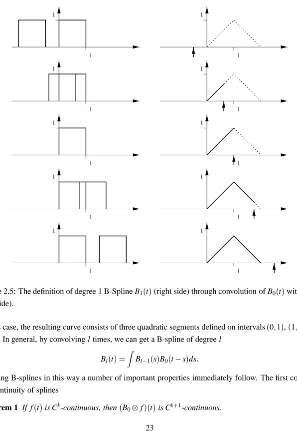
1 1 1 1 1 1 1 1 1 1 1 1 1 1 1 1 1 1 1 1

Figure 2.5: The definition of degree 1 B-Spline B

1(

t

)

(right side) through convolution of B

0(

t

)

with itself

(left side).

In this case, the resulting curve consists of three quadratic segments defined on intervals

(

0

;

1

)

,

(

1

;

2

)

and

(

2

;

3

)

. In general, by convolving l times, we can get a B-spline of degree l

B

l(

t

)= Z

B

l,1

(

s

)

B

0(

t

,

s

)

ds

:

Defining B-splines in this way a number of important properties immediately follow. The first concerns

the continuity of splines

Theorem 1 If f

(

t

)

is C

k

_{-continuous, then}

(

B

0

f

)(

t

)

is C

k+1

(24)

This is a direct consequence of convolution with a box function. From this it follows that the B-spline of

degree n is C

n,1

continuous because the B-spline of degree 1 is C

0

-continuous.

2.2.3 Refinability of B-splines

Another remarkable property of B-splines is that they obey a refinement equation. This is the key

observation to connect splines and subdivision. The refinement equation for B-splines of degree l is

given by

B

l(

t

)=

1

2

l l+1

∑

k=0

l

+

1 k

B

l(

2t

,

k

):

(2.1)

In other words, the B-spline of degree l can be written as a linear combination of translated (k) and

dilated (2t) copies of itself. For a function to be refineable in this way is a rather special property. As an

example of the above equation at work consider the hat function shown in Figure 2.5. It is easy to see that

it can be written as a linear combination of dilated hat functions with weights

(

1

=

2

;

1

;

1

=

2

)

respectively.

The property of refinability is the key to subdivision and so we will take a moment to prove it. We

start by observing that the box function, i.e., the B-spline of degree 0 can be written in terms of dilates

and translates of itself

B

0(

t

)=

B

0(

2t

)+

B

0(

2t

,

1

);

(2.2)

which is easily checked by direct inspection. Recall that we defined the B-spline of degree l as

B

l(

t

)= l O i=0

B

0(

t

)= l O i=0 (

B

0(

2t

)+

B

0(

2t

,

1

))

(2.3)

This expression can be “multiplied” out by using the following properties of convolution for functions

f

(

t

)

, g

(

t

)

, and h

(

t

)

f

(

t

)(

g

(

t

)+

h

(

t

)) =

f

(

t

)

g

(

t

)+

f

(

t

)

h

(

t

)

linearity

f

(

t

,

i

)

g

(

t

,

k

) =

m

(

t

,

i

,

k

)

time shift

f

(

2t

)

g

(

2t

) = 1 2

m

(

2t

)

time scaling

where m

(

t

)=

f

(

t

)

g

(

t

)

. These properties are easy to check by substituting the definition of convolution

(25)

For example, in the case of B

1

we get

B

1(

t

) =

B

0(

t

)

B

0(

t

) = (

B

0(

2t

)+

B

0(

2t

,

1

))(

B

0(

2t

)+

B

0(

2t

,

1

)) =

B

0(

2t

)

B

0(

2t

)+

B

0(

2t

)

B

0(

2t

,

1

)+

B

0(

2t

,

1

)

B

0(

2t

)+

B

0(

2t

,

1

)

B

0(

2t

,

1

) =

1

2 B

1(

2t

)+

1

2 B

1(

2t

,

1

)+

1

2 B

1(

2t

,

1

)+

1

2 B

1(

2t

,

1

,

1

) =

1

2

(

B

1(

2t

)+

2B

1(

2t

,

1

)+

B

1(

2t

,

2

)) =

1

2

1 2

∑

k=0

2 k

B

1(

2t

,

k

):

The general statement for B-splines of degree l now follows from the binomial theorem

(

x

+

y

) l+1 = l+1

∑

k=0

l

+

1 k

x

l+1,k

y

k;

with B

0(

2t

)

in place of x and B

0(

2t

,

1

)

in place of y.

2.2.4 Refinement for Spline Curves

With this machinery in hand let’s revisit spline curves. Let

γ

(

t

)= "

x

(

t

)

y

(

t

) # =

∑

i

p

i

B

il(

t

)

be such a spline curve of degree l with control points

(

x

i;

y

i) T

=

p

i2

R

2

_{. Since we don’t want to worry}

about boundaries for now we leave the index set i unspecified. We will also drop the subscript l since the

degree, whatever it might be, is fixed for all our examples. Due to the definition of B

i(

t

)=

B

(

t

,

i

)

each

control point exerts influence over a small part of the curve with parameter values t

2[

i

;

i

+

l

]

.

Now consider p, the vector of control points of a given curve:

p

= 2 6 6 6 6 6 6 6 6 6 6 6 6 4

..

.

p,

2

p,

1

p

0

p

1

p

2

..

.

3 7 7 7 7 7 7 7 7 7 7 7 7 5

(26)

and the vector B

(

t

)

, which has as its elements the translates of the function B as defined above

B

(

t

)= h :::

B

(

t

+

2

)

B

(

t

+

1

)

B

(

t

)

B

(

t

,

1

)

B

(

t

,

2

) ::: i :

In this notation we can denote our curve as B

(

t

)

p.

Using the refinement relation derived earlier, we can rewrite each of the elements of B in terms of its

dilates

B

(

2t

)= h :::

B

(

2t

+

2

)

B

(

2t

+

1

)

B

(

2t

)

B

(

2t

,

1

)

B

(

2t

,

2

) ::: i ;

using a matrix S to encode the refinement equations

B

(

t

)=

B

(

2t

)

S

:

The entries of S are given by Equation 2.1

S

2i+k;i =

s

k=

1

2

l

+

1 k

:

The only non-zero entries in each column are the weights of the refinement equation, while successive

columns are copies of one another save for a shift down by two rows.

We can use this relation to rewrite

γ

(

t

)

γ

(

t

)=

B

(

t

)

p

=

B

(

2t

)

Sp

:

It is still the same curve, but desribed with respect to dilated B-splines, i.e., B-splines whose support is

half as wide and which are spaced twice as dense. We performed a change from the old basis B

(

t

)

to the

new basis B

(

2t

)

and concurrently changed the old control points p to the appropriate new control points

Sp. This process can be repeated

γ

(

t

) =

B

(

t

)

p

0 =

B

(

2t

)

p

1 =

B

(

2t

)

Sp

0

..

.

=

B

(

2

j

_t

)

p

j =

B

(

2

j

_t

)

S

j

_p

0 ;

from which we can define the relationship between control points at different levels of subdivision

p

j+1 =

Sp

j ;

(27)

Looking more closely at one component, i, of our control points we see that

p

j+1 i =

∑

l

S

i;l

p

j l:

To find out exactly which s

k

is affecting which term, we can divide the above into odd and even entries.

For the odd entries we have

p

j+1 2i+1 =

∑

l

S

2i+1;l

p

j l =

∑

l

s

₂(i,l)+1

p

j l

and for the even entries we have

p

j+1 2i =

∑

l

S

2i;l

p

j l =

∑

l

s

2(i,l)

p

j l:

From which we essentially get two different subdivision rules one for the new even control points of the

curve and one for the new odd control points. As examples of the above, let us consider two concrete

cases. For piecewise linear subdivision, the basis functions are hat functions. The odd coefficients are

1₂

and

1₂

, and a lone 1 for the even point. For cubic splines the odd coefficients turn out to be

1₂

and

1₂

, while

the even coefficients are

1₈

,

6₈

, and

1₈

.

Another way to look at the distinction between even and odd is to notice that odd points at level j

+

1 are newly inserted, while even points at level j

+

1 correspond directly to the old points from level j.

In the case of linear splines the even points are in fact the same at level j

+

1 as they were at level j.

Subdivision schemes that have this property will later be called interpolating, since points, once they

have been computed, will never move again. In contrast to this consider cubic splines. In that case even

points at level j

+

1 are local averages of points at level j so that p

j+1 2i 6=

p

j

i

. Schemes of this type will

later be called approximating.

2.2.5 Subdivision for Spline Curves

In the previous section we saw that we can refine the control point sequence for a given spline by

multi-plying the control point vector p by the matrix S, which encodes the refinement equation for the B-spline

used in the definition of the curve. What happens if we keep repeating this process over and over,

gen-erating ever denser sets of control points? It turns out the control point sequence converges to the actual

spline curve. The speed of convergence is geometric, which is to say that the difference between the

curve and its control points decreases by a constant factor on every subdivision step. Loosely speaking

this means that the actual curve is hard to distinguish from the sequence of control points after only a

few subdivision steps.

(28)

We can turn this last observation into an algorithm and the core of the subdivision paradigm. Instead

of drawing the curve itself on the screen we draw the control polygon, i.e., the piecewise linear curve

through the control points. Applying the subdivision matrix to the control points defines a sequence of

piecewise linear curves which quickly converge to the spline curve itself.

In order to make these observations more precise we need to introduce a little more machinery in the

next section.

2.3 Subdivision as Repeated Refinement

2.3.1 Discrete Convolution

The coefficients s

k

of the B-spline refinement equation can also be derived from another perspective,

namely discrete convolution. This approach mimics closely the definition of B-splines through

continu-ous convolution. Using this machinery we can derive and check many useful properties of subdivision

by looking at simple polynomials.

Recall that the generating function of a sequence a

k

is defined as

A

(

z

)=

∑

k

a

k

z

k;

where A

(

z

)

is the z-transform of the sequence a

k

. This representation is closely related to the discrete

Fourier transform of a sequence by restricting the argument z to the unit circle, z

=

exp

(

i

θ

)

. For the case

of two coefficient sequences a

k

and b

k

their convolution is defined as

c

k=(

a

b

)k=

∑

n

a

k,n

b

n :

In terms of generating functions this can be stated succinctly as

C

(

z

)=

A

(

z

)

B

(

z

);

which comes as no surprise since convolution in the time domain is multiplication in the Fourier domain.

The main advantage of generating functions, and the reason why we use them here, is that

manip-ulations of sequences can be turned into simple operations on the generating functions. A very useful

example of this is the next observation. Suppose we have two functions that each satisfy a refinement

equation

f

(

t

) =

∑

k

a

k

f

(

2t

,

k

)

g

(

t

) =

∑

k

b

k

g

(

2t

,

k

):

(29)

In that case the convolution h

=

f

g of f and g also satisfies a refinement equation

h

(

t

)=

∑

k

c

k

h

(

2t

,

k

);

whose coefficients c

k

are given by the convolution of the coefficients of the individual refinement

equa-tions

c

k=

1

2 ∑

_i

a

k,i

b

i :

With this little observation we can quickly find the refinement equation, and thus the coefficients of the

subdivision matrix S, by repeated multiplication of generating functions. Recall that the box function

B

0(

t

)

satisfies the refinement equation B

0(

t

)=

B

0(

2t

)+

B

0(

2t

,

1

)

. The generating function of this

refinement equation is A

(

z

)=(

1

+

z

)

since the only non-zero terms of the refinement equation are those

belonging to indices 0 and 1. Now recall the definition of B-splines of degree l

B

l(

t

)= l O k=0

B

0(

t

);

from which we immediately get the associated generating function

S

(

z

)=

1

2

l(

1

+

z

)

l+1 :

The values s

k

used for the definition of the subdivision matrix are simply the coefficients of the various

powers of z in the polynomial S

(

z

)

S

(

z

)=

1

2

l l+1

∑

k=0

l

+

1 k

z

k;

where we used the binomial theorem to expand S

(

z

)

. Note how this matches the definition of s

k

in

Equation 2.1.

Recall Theorem 1, which we used to argue that B-splines of degree n are C

n,1

continuous. That same

theorem can now be expressed in terms of generating functions as follows

Theorem 2 If S

(

z

)

defines a convergent subdivision scheme yielding a C

k

_{-continuous limit function then}

1

2(

1

+

z

)

S

(

z

)

defines a convergent subdivision scheme with C

k+1

-continuous limit functions.

We will put this theorem to work in analyzing a given subdivision scheme by peeling off as many

fac-tors of

1₂(

1

+

z

)

as possible, while still being able to prove that the remainder converges to a continuous

(30)

limit function. With this trick in hand all we have left to do is establish criteria for the convergence of

a subdivision scheme to a continuous function. Once we can verify such a condition for the

subdivi-sion scheme associated with B-spline control points we will be justified in drawing the piecewise linear

approximations of control polygons as approximations for the spline curve itself. We now turn to this

task.

2.3.2 Convergence of Subdivision

There are many ways to talk about the convergence of a sequence of functions to a limit. One can use

different norms and different notions of convergence. For our purposes the simplest form will suffice,

uniform convergence.

We say that a sequence of functions f

i

defined on some interval

[

a

;

b

]

R converges uniformly to a

limit function f if for all

ε

>

0 there exists an n

0>

0 such that for all n

>

n

0

max

t2[a;b]

j

f

(

t

),

f

n(

t

)j<

ε

:

Or in words, as of a certain index (n

0

) all functions in the sequence “live” within an

ε

sized tube around

the limit function f . This form of convergence is sufficient for our purposes and it has the nice

prop-erty that if a sequence of continuous functions converges uniformly to some limit function f , that limit

function is itself continuous.

For later use we introduce some norm symbols

k

f

(

t

)k =

sup

t j

f

(

t

)j k

p

k =

sup

i j

p

ij k

S

k =

sup

i

∑

_k j

S

ikj;

which are compatible in the sense that, for example,

k

Sp

kk

S

kk

p

k

.

The sequence of functions we want to analyze now are the control polygons as we refine them with

the subdivision rule S. Recall that the control polygon is the piecewise linear curve through the control

points p

j

at level j. Independent of the subdivision rule S we can use the linear B-splines to define the

piecewise linear curve through the control points as P

j(

t

)=

B

1(

2

j

_t

)

p

j

_.

One way to show that a given subdivision scheme S converges to a continuous limit function is to

prove that (1) the limit

P

∞(

t

)=

lim

j!∞

(31)

exists for all t and (2) that the sequence P

j(

t

)

converges uniformly. In order to show this property we

need to make the assumption that all rows of the matrix S sum to 1, i.e., the odd and even coefficients of

the refinement relation separately sum to 1. This is a reasonable requirement since it is needed to ensure

the affine invariance of the subdivision process, as we will later see. In matrix notation this means S1

=

1,

or in other words, the vector of all 1’s is an eigenvector of the subdivision matrix with eigenvalue 1. In

terms of generating functions this means S

(,

1

)=

0, which is easily verified for the generating functions

we have seen so far.

Recall that the definition of continuity in the function setting is based on differences. We say f

(

t

)

is continuous at t

0

if for any

ε

>

0 there exists a

δ

>

0 so that

j

f

(

t

0),

f

(

t

)j<

ε

as long as

j

t

0,

t

j<

δ

.

The corresponding tool in the subdivision setting is the difference between two adjacent control points

p

_ij +1 ,

p

j i =(

∆

p

j

)i

. We will show that if the differences between neighboring control points shrink fast

enough, the limit curve will exist and be continuous:

Lemma 3 If

k

∆

p

j

k<

c

γ

j

_{for some constant c}

>

0 and a shrinkage factor 0

<

γ

<

1 for all j

>

j

0

0 then P

j(

t

)

converges to a continuous limit function P

∞

(

t

)

.

Proof: Let S be the subdivision rule at hand, p

1=

Sp

0

_{and S}

1

be the subdivision rule for B-splines of

degree 1. Notice that the rows of S

,

S

1

sum to 0

(

S

,

S

1)

1

=

S1

,

S

1

=

1

,

1

=

0

:

This implies that there exists a matrix D such that S

,

S

1=

D

∆

, where

∆

computes the difference of

adjacent elements

(

∆

)ii=,

1,

(

∆

)i ;i+1

=

1, and zero otherwise. The entries of D are given as D

i j = ,

∑

j k=i

(

S

,

S

1)ik

. Now consider the difference between two successive piecewise linear approximations

of the control points

k

P

j+1 (

t

),

P

j (

t

)k = k

B1

(

2

j+1

t

)

p

j+1 ,

B1

(

2

j

_t

)

p

j k = k

B1

(

2

j+1

t

)

Sp

j ,

B1

(

2

j+1

t

)

S

1

p

j k = k

B

1(

2

j+1

t

)(

S

,

S

1)

p

j k k

B

1(

2

j+1

t

)kk

D

∆

p

j k k

D

kk

∆

p

j k k

D

k

c

γ

j :

This implies that the telescoping sum P

0(

t

)+

∑

j k=0 (

P

k+1 ,

P

k

)(

t

)

converges to a well defined limit

func-tion since the norms of each summand are bounded by a constant times a geometric term

γ

j

_{. Let P}

∞ (

t

)

(32)

as j

!

∞

, then

k

P

∞ (

t

),

P

j (

t

)k< k

D

k

c

1

,

γ

j ;

since the latter is the tail of a geometric series. This implies uniform convergence and thus continuity of

P

∞(

t

)

as claimed.

How do we check such a condition for a given subdivision scheme? Suppose we had a derived

subdivision scheme D for the differences themselves

∆

p

j+1

=

D

∆

p

j

;

defined as the scheme that satisfies

∆

S

=

D

∆

:

Or in words, we are looking for a difference scheme D such that taking differences after subdivision is

the same as applying the difference scheme to the differences. Does D always exist? The answer is yes

if S is affinely invariant, i.e., S

(,

1

)=

0. This follows from the following argument. Multiplying S by

∆

computes a matrix whose rows are differences of adjacent rows in S. Since odd and even numbered rows

of S each sum to one, the rows of

∆

S must each sum to zero. Now the existence of a matrix D such that

∆

S

=

D

∆

follows as in the argument above.

Given this difference scheme D all we would have to show is that some power m

>

0 of D has norm

less than 1,

k

D

m k=

γ

<

1. In that case

k

∆

p

j k<

c

(

γ

1=m )

j

_{. (We will see in a moment that the extra degree}

of freedom provided by the parameter m is needed in some cases.)

As an example, let us check this condition for cubic B-splines. Recall that B

3(

z

)= 1 8(

1

+

z

) 4

_{, i.e.,}

p

j+1 2i+1 =

1

8

(

4p

j i +

4p

j i+1 )

p

j+1 2i =

1

8

(

p

j i,1 +

6p

j i+

p

j i+1 ):

Taking differences we have

(

∆

p

j+1 )2i =

p

j+1 2i+1 ,

p

j+1 2i =

1

8

(,

p

j i,1 ,

2p

j i +

3p

j i+1 ) =

1

8

(

3

(

p

j i+1 ,

p

j i)+

1

(

p

j i,

p

j i,1 ))=

1

8

(

3

(

∆

p

j )i+

1

(

∆

p

j )i ,1 );

and similarly for the odd entries so that D

(

z

)= 1 8(

1

+

z

)

3

_{, from which we conclude that}

k

D

k=

1

2

, and that

the subdivision scheme for cubic B-splines converges uniformly to a continuous limit function, namely

the B-spline itself.

(33)

Another example, which is not a spline, is the so called 4 point scheme [5]. It was used to create

the curve in Figure 2.1, which is interpolating rather than approximating as is the case with splines. The

generating function for the 4 point scheme is

S

(

z

)=

1

16

(,

z

,3 +

4z

,2 ,

z

,1 )(

1

+

z

) 4

Recall that each additional factor of

1₂(

1

+

z

)

in the generating function increases the order of continuity of

the subdivision scheme. If we want to show that the limit function of the 4 point scheme is differentiable

we need to show that

1₈(,

z

,3 +

4z

,2 ,

z

,1 )(

1

+

z

)

3

_{converges to a continuous limit function. This in}

turn requires that D

(

z

)= 1 8(,

z

,3 +

4z

,2 ,

z

,1 )(

1

+

z

)

2

_{satisfy a norm estimate as before. The rows of D}

have non-zero entries of

( 1 4; 1 4)

, and

( ,1 8 ; 6 8; ,1

8 )

respectively. Thus

k

D

k=

1, which is not strong enough.

However, with a little bit more work one can show that

k

D

2

k= 3

4

, so that indeed the 4 point scheme is

C

1

.

In general, the difficult part is to find a set of coefficients for which subdivision converges. There

is no general method to achieve this. Once a convergent subdivision scheme is found, one can always

obtain a desired order of continuity by convolving with the box function.

2.3.3 Summary

So far we have considered subdivision only in the context of splines where the subdivision rule, i.e., the

coefficients used to compute a refined set of control points, was fixed and everywhere the same. There

is no pressing reason for this to be so. We can create a variety of different curves by manipulating the

coefficients of the subdivision matrix. This could be done globally or locally. I.e., we could change the

coefficients within a subdivision level and/or between subdivision levels. In this regard, splines are just

a special case of the more general class of curves, subdivision curves. For example, at the beginning of

this chapter we briefly outlined an interpolating subdivision method, while spline based subdivision is

approximating rather than interpolating.

Why would one want to draw a spline curve by means of subdivision? In fact there is no sufficiently

strong reason for using subdivision in one dimension and none of the commercial line drawing packages

do so, but the argument becomes much more compelling in higher dimensions as we will see in later

chapters.

In the next section we use the subdivision matrix to study the behavior of the resulting curve at a point

or in the neighborhood of a point. We will see that it is quite easy, for example, to evaluate the curve

exactly at a point, or to compute a tangent vector, simply from a deeper understanding of the subdivision

matrix.

(34)

2.4 Analysis of Subdivision

In the previous section we have shown that uniform spline curves can be thought of as a special case of

subdivision curves. So far, we have seen only examples for which we use a fixed set of coefficients to

compute the control points everywhere. The coefficients define the appearance of the curve, for example,

whether it is differentiable or has sharp corners. Consequently it is possible to control the appearance of

the curve by modifying the subdivision coefficients locally. So far we have not seen a compelling reason

to do so in the 1D setting. However, in the surface setting it will be essential to change the subdivision

rule locally around extraordinary vertices to ensure maximal order of continuity. But before studying this

question we once again look at the curve setting first since the treatment is considerably easier to follow

in that setting.

To study properties such as differentiability of the curve (or surface) we need to understand which

of the control points influences the neighborhood of the point of interest. This notion is captured by the

concept of invariant neighborhoods to which we turn now.

2.4.1 Invariant Neighborhoods

Suppose we want to study the limit curve of a given subdivision scheme in the vicinity of a particular

control point.

3

To determine local properties of a subdivision curve, we do not need the whole infinite

vector of control points or the infinite matrix describing subdivision of the entire curve. Differentiability,

for example, is a local property of a curve. To study it we need consider only an arbitrarily small piece

of the curve around the origin. This leads to the question of which control points influence the curve in

the neighborhood of the origin?

As a first example consider cubic B-spline subdivision. There is one cubic segment to the left of the

origin with parameter values t

2[,

1

;

0

]

and one segment to the right with parameter range t

2[

0

;

1

]

.

Figure 2.6 illustrates that we need 5 control points at the coarsest level to reach any point of the limit

curve which is associated with a parameter value between

,

1 and 1, no matter how close it is to the

origin. We say that the invariant neighborhood has size 5. This size depends on the number of non-zero

entries in each row of the subdivision matrix, which is 2 for odd points and 3 for even points. The latter

implies that we need one extra control point to the left of

,

1 and one to the right of 1.

Another way to see this argument is to consider the basis functions associated with a given subdivision

scheme. Once those are found we can find all basis functions overlapping a region of interest and

3_{Here and in the following we assume that the point of interest is the origin. This can always be achieved through}