Plant high-throughput phenotyping using photogrammetry and 3D modeling techniques

(1)

PLANT HIGH-THROUGHPUT PHENOTYPING USING PHOTOGRAMMETRY AND 3D MODELING TECHNIQUES

by NAN AN

M.A., University of Kansas, 2009

B.S., China University of Geosciences, Beijing, 2005 AN ABSTRACT OF A DISSERTATION

submitted in partial fulfillment of the requirements for the degree

DOCTOR OF PHILOSOPHY

Department of Agronomy College of Agriculture

KANSAS STATE UNIVERSITY Manhattan, Kansas

(2)

Abstract

Plant phenotyping has been studied for decades for understanding the relationship between plant genotype, phenotype, and the surrounding environment. Improved accuracy and efficiency in plant phenotyping is a critical factor in expediting plant breeding and the selection process. In the past, plant phenotypic traits were extracted using invasive and destructive

sampling methods and manual measurements, which were time-consuming, labor-intensive, and cost-inefficient. More importantly, the accuracy and consistency of manual methods can be highly variable. In recent years, however, photogrammetry and 3D modeling techniques have been introduced to extract plant phenotypic traits, but no cost-efficient methods using these two techniques have yet been developed for large-scale plant phenotyping studies. High-throughput 3D modeling techniques in plant biology and agriculture are still in the developmental stages, but it is believed that the temporal and spatial resolutions of these systems are well matched to many plant phenotyping needs. Such technology can be used to help rapid phenotypic trait extraction aid crop genotype selection, leading to improvements in crop yield.

In this study, we introduce an automated high-throughput phenotyping pipeline using affordable imaging systems, image processing, and 3D reconstruction algorithms to build 2D mosaicked orthophotos and 3D plant models. Chamber-based and ground-level field

implementations can be used to measure phenotypic traits such as leaf length, rosette area in 2D and 3D, plant nastic movement, and diurnal cycles. Our automated pipeline has cross-platform capabilities and a degree of instrument independence, making it suitable for various situations.

(3)

PLANT HIGH-THROUGHPUT PHENOTYPING USING PHOTOGRAMMETRY AND 3D MODELING TECHNIQUES

by NAN AN

M.A., University of Kansas, 2009

B.S., China University of Geosciences, Beijing, 2005 A DISSERTATION

submitted in partial fulfillment of the requirements for the degree

DOCTOR OF PHILOSOPHY Department of Agronomy

College of Agriculture

KANSAS STATE UNIVERSITY Manhattan, Kansas 2015 Approved by: Co-Major Professor Stephen Welch Approved by: Co-Major Professor Kevin Price

(4)

Copyright

NAN AN

(5)

Abstract

Plant phenotyping has been studied for decades for understanding the relationship between plant genotype, phenotype, and the surrounding environment. Improved accuracy and efficiency in plant phenotyping is a critical factor in expediting plant breeding and the selection process. In the past, plant phenotypic traits were extracted using invasive and destructive

sampling methods and manual measurements, which were time-consuming, labor-intensive, and cost-inefficient. More importantly, the accuracy and consistency of manual methods can be highly variable. In recent years, however, photogrammetry and 3D modeling techniques have been introduced to extract plant phenotypic traits, but no cost-efficient methods using these two techniques have yet been developed for large-scale plant phenotyping studies. High-throughput 3D modeling techniques in plant biology and agriculture are still in the developmental stages, but it is believed that the temporal and spatial resolutions of these systems are well matched to many plant phenotyping needs. Such technology can be used to help rapid phenotypic trait extraction aid crop genotype selection, leading to improvements in crop yield.

In this study, we introduce an automated high-throughput phenotyping pipeline using affordable imaging systems, image processing, and 3D reconstruction algorithms to build 2D mosaicked orthophotos and 3D plant models. Chamber-based and ground-level field

implementations can be used to measure phenotypic traits such as leaf length, rosette area in 2D and 3D, plant nastic movement, and diurnal cycles. Our automated pipeline has cross-platform capabilities and a degree of instrument independence, making it suitable for various situations.

(6)

List of Figures

Figure 1.1 Potted Arabidopsis thaliana plant. ... 12

Figure 1.2. Flowchart of the high-throughput phenotyping pipeline. ... 13

Figure 2.1 Original image with optical distortion and perspective distortion. ... 44

Figure 2.2 Image analysis workflow. ... 45

Figure 2.3 Indoor imaging platform. ... 46

Figure 2.4 Field imaging platform. ... 47

Figure 2.5 Field image data management. ... 48

Figure 2.6 Orthophoto processing... 49

Figure 2.7 Field single plant extraction and genotype assignment. ... 50

Figure 2.8 Image optical distortion correction. ... 51

Figure 2.9 Image color correction. ... 52

Figure 2.10 Image perspective correction. ... 53

Figure 2.11 Indoor orthophoto-rendering methods comparison. ... 54

Figure 2.12 Field orthophoto-rendering methods comparison. ... 55

Figure 2.13 First iteration of leaf tip detection. ... 56

Figure 2.14 Second iteration of leaf tip detection. ... 57

Figure 2.15 Relationship of rosette area and total leaf expansion for indoor environment ... 58

Figure 2.16 Parameter estimations for indoor environment. ... 59

Figure 2.17 Relationship of rosette area and total leaf expansion for field environment. ... 60

Figure 2.18 Parameter estimations for field environment. ... 61

Figure 2.19 Original image and analyzed image of the outlier. ... 62

Figure 3.1 Camera calibration... 86

Figure 3.2 A half-shelf 3D mesh generated by Photoscan... 87

Figure 3.3 Single-plant binary image for extracting a single-plant 3D model. ... 88

Figure 3.4 A single-plant vertex map. ... 89

Figure 3.5 A single-plant 3D model. ... 90

Figure 3.6 Plant orthophoto vs. 3D model. ... 91

Figure 3.7 Half-shelf 3D mesh before and after camera calibration. ... 92

(10)

Figure 3.9 Time-series 3D models. ... 94 Figure 3.10 Z score comparison between 3D area and 2D area. ... 95

(11)

List of Tables

Table 2.1 Throughput capability of chamber phenotyping processing pipeline. ... 63

Table 2.2 The statistics of the parameter estimation for indoor environment. ... 64

Table 2.3 The statistics of the parameter estimation for field environment. ... 65

Table 3.1 Sample Python code for sorting and extracting plant vertices and faces. ... 96

(12)

Acknowledgements

I owe a great amount of appreciation to a large number of people who helped me complete my dissertation and guided my career path instrumentally and emotionally.

I would like to express my deepest gratitude to my advisors, mentors, and friends, Dr. Stephen Welch and Dr. Kevin Price. Thank both of you so much for your unconditional support that made it possible for me to complete my dissertation. I will always remember the personal and professional interactions we had over the years. I am grateful for the influence of your personalities and your attitudes on my career, family, and life in general. Both of you not only taught me critical thinking skills as a researcher but also taught me how to reflect and learn from each life experience. I will remember the teachings from both of you for the rest of my life.

I would also like to thank my committee members: Dr. Jesse Poland, Dr. Stephen Egbert, and Dr. Stacy Hutchinson. Your invaluable feedback and suggestions encouraged me to broaden my horizons so I could incorporate them into my dissertation. I would also love to thank Dr. Cynthia Weinig at the University of Wyoming and Dr. Julin Maloof at the University of California, Davis for their support on my project.

I appreciate all of the help and suggestions from my collaborators: Christine Palmer, Robert Baker, Cody Markelz, James Ta, Smita Sharan, Rishab Vaswani, Lakshmi Narjala, Wen Fung Leong, and Huan Wang. All of you provided invaluable help throughout years on this project.

Last but not least, I especially want to thank my parents for believing in me and giving me the autonomy to pursue my dreams. Without your numerous sacrifices and support, I would not have been able to complete my Ph.D. and enjoy my personal and professional growth. To my supportive wife, life partner, and soul mate, Ran Zhao, thank you for standing by me through all

(13)

these seven years. I am glad that we have each other to witness many of our life milestones and have shared our laughter and tears together in the past nine years. I am also grateful for the joy, excitement, hope, and love as a father that Dillon and Ian (on the way) have brought to me. Seeing your smile is the most beautiful thing of all.

(14)

Dedication

For my parents My beautiful wife, Ran Zhao And my lovely boys, Dillon and Ian

(15)

Chapter 1 - Introduction

Plant high-throughput phenotyping

Phenotyping is acquiring a set of observable characteristics of plants resulting from the interaction of their genotypes with the environment (Wanscher 1975; Blum et al. 1982). Traditional phenotyping methods often rely on simple tools like rulers and other measuring devices, along with large amounts of manual work, to extract the desired trait data. Compared to advanced genotyping methods such as the latest sequencing technologies, traditional

phenotyping methods are time-consuming, labor-intensive, and cost-inefficient. This limits our ability to quantitatively understand how genetic traits are related to plant growth, environmental adaptation, and yield.

In the past several years, tremendous interest in plant high-throughput phenotyping (HTP) techniques has arisen. These techniques use sensor systems and automated computer algorithms to extract phenotypic traits for large genetic mapping populations using non-destructive and non-invasive sampling methods (Fiorani and Schurr 2013). With such new techniques, plant phenotypes can be linked with functional genomics and environmental factors, thus facilitating plant breeding and leading toward improved crop production and yield stability. This is essential to meet the expected demands of the world population by 2050 (Bolon et al. 2011; Bongaarts 2014).

Typically, the extraction of data via HTP methods involves a series of discrete steps that must be reliably executed in sequence. Such a set of steps is referred to as a “pipeline”.

Commercial phenotyping systems such as GROWSCREEN⁄FLUORO (Walter et al. 2007; Jansen et al. 2009), PHENOPSIS (Granier et al. 2006), and the LemnaTec Scanalyzer HTS

(16)

(Furbank and Tester 2011; Green et al. 2012; Chen et al. 2014; Dornbusch et al. 2014) have been used in some small-scale research laboratories for automating plant phenotyping in controlled environments. Larger-scale, fully-automated high-throughput phenotyping facilities have also been deployed in the greenhouses or growth chambers of private sector firms such as Monsanto and Dupont Pioneer and in the most advanced national plant research institutions such as the Australian Plant Phenomics Facility, the European Plant Phenotyping Network, and USDA; however, these indoor facilities cannot be used for field phenotyping. Additionally, the cost of these systems is beyond most research laboratories’ budgets, thus slowing the advance of science.

In the field, most phenotyping systems have mainly focused on automated solutions for data acquisition using platforms that combine a vehicle and perhaps some robotics with imaging systems and sensors. Less well-developed are complete data pipelines that automate data storage, processing, and analysis (White et al. 2012). The result can be that slow manual collection of small amounts of data is replaced by slow manual management of large amounts of

automatically-collected data. Therefore, what is needed is integrated HTP and data management systems incorporating both data acquisition and processing. Ideally, these systems would be sufficiently generic to be used with minimal or no alteration in both laboratory and field settings. We will present such a system in this and the chapters that follow, but first we will describe the biological system of interest.

The model plant

Arabidopsis thaliana

The plant used as the test subject in this study is Arabidopsis thaliana (L.) Heynh. It is a small, rapidly maturing plant in the Brassicaceae that is native to Europe, Asia, and parts of North Africa. It has also invaded North America on several occasions and is, therefore, virtually

(17)

ubiquitous from latitude 25 to 65 N, except for Greenland. It is also found in parts of South America, Sub-Saharan Africa, Australia, and New Zealand. Arabidopsis thaliana is an important model system that has been used for identifying plant genes and determining their functions (Arabidopsis Genome Initiative, 2000). It has a small genome and its small stature and rapid development times make it an ideal genetic model plant for the same reasons that Drosophila is an ideal genetic model for animals. It was the first plant to have its genome sequenced (in 2000).

Figure 1.1 shows an Arabidopsis plant with key parts labeled. This study primarily focuses on vegetative development and the critical phenotypes are the areas, lengths, and angles of the rosette leaves, which form a circular pattern in close proximity to the ground.

Shade-avoidance responses

All plants are vulnerable to shading by taller neighbors and this is particularly so in Arabidopsis because its rosette is close to the ground. Shade-avoidance behaviors form a suite of responses that plants can undertake to find more light. They range from increased leaf

elongation, alteration of leaf angles, growth in a more upward rather than outward direction, and even flowering more rapidly (Morelli and Ruberti 2000; Mullen et al. 2006).

Shade-avoidance responses are triggered by the reduced amounts of photosynthetically active radiation (PAR) transmitted through or reflected from plant tissues. In plant leaves, chlorophyll absorbs light more strongly in the red portion of the spectrum than in the longer-wavelength, far-red region (Smith, 1982). Phytochrome is an important plant pigment that has two molecular configurations that are differentially sensitive to these two wavebands; therefore, the plant is able to sense the ratio of red to far-red wavelengths (R: FR). Low ratios are an accurate signal of neighboring plant proximity and, therefore, a positive indicator of competitive intensity (Ballare et al. 1990; Smith et al. 1990; Gilbert et al. 2001; Schmitt et al. 2003). Thus,

(18)

shade-avoidance phenotypes constitute an interesting complex of traits whose intricate

interactions with each other and with the environment are therefore widely studied (Weijschedé et al. 2006; Schmitt et al. 2003).

As listed above, leaf length, rosette area, and leaf angles are widely-studied traits related to shade-avoidance responses. Chitwood et al. (2012) manipulated far-red light to induce changes in leaf length. This study found a linear relationship between total leaf length and the square root of total leaf area. This study involved destructive sampling of fully-developed leaves. Studies of leaf angles are not only important in shade avoidance but also in studies of repetitive daily patterns of activity. Under some circumstances, plant leaves can rise and fall in an

oscillatory behavior that can serve as a proxy for the cycling of the plant’s circadian clock (Hong et al. 2013; Dornbusch et al. 2014). In indoor environments (although not in the field),

Arabidopsis plants exhibit these nastic movements (Greenham et al. 2015).

In many shade-avoidance and growth-stage related studies, leaf area, leaf length and rosette area were obtained using mechanical measuring tools, such as calipers or rulers (Poethig and Sussex 1985; Boyes et al. 2001; Weijschedé et al. 2006, Gonzalez et al. 2010). The accuracy of those data, however, is limited by systematic error from the precision of conventional

measuring tools along with human errors during invasive plant handling and subjective interpretation. The manual measurement process is also time-consuming and labor-intensive. Arvidsson et al. (2011) indicated a major bias in that the measurements of one stage during a particular plant developmental period are insufficient to interpret the phenotypes at other stages. Therefore, continuous time-series measurements during the entire developmental period are needed for studying shade-avoidance traits and, presumably, for other types of plant

(19)

Objectives

In the HTP pipeline to be described, the three traits of total leaf length, leaf area, and leaf angle will be detected by both 2D and 3D processing in a laboratory environment. The first two will also be monitored in the field using the 2D components of the same pipeline.

This pipeline is low-cost, fully-automated, and, as just noted, generic. That is, the

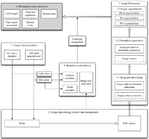
pipeline was specifically designed at the application level to have cross-platform capabilities and a degree of instrument independence. As depicted by the flowchart shown in Figure 1.2, the pipeline contains five sections. 1) Image data acquisition used different platforms in indoor vs. field environments to collect time-series images of plant development. Indoor, stationary imaging systems were designed and mounted on each of six shelves in a growth chamber of University of California, Davis (UCD). At the University of Wyoming (UWY), a mobile imaging system was developed for use in the field. 2) Image data storage, transmission, and management involved the use of servers at UCD, UWY, and Kansas State University (KSU). For both the chamber and field experiments, images were stored locally and then transmitted via the iPlant Collaborative (http://www.iplantcollaborative.org/) (iPlant) to servers at KSU. This resulted in three complete backups of all image sets: one at the origin, one at iPlant, and one at KSU. 3) Image processing operations include pre-processing, orthophoto generation, and image segmentation. 4) Metadata reconciliation is necessary because metadata generated by different sources (i.e., human-entered data and/or some automated data) may conflict regarding the identity of each image. Reconciliation yields the most accurate pairings of genotype and phenotype data. 5) Phenotype extraction includes the machine-vision operations that yield the biological data that comprise the ultimate goal of the system. Python, a high-level scripting language, was used to connect and automate the sections.

(20)

In Chapter 2, we develop the pipeline in the context of a growth chamber experiment. It extracts data on total leaf length and 2D rosette area for a set of 1050 distinct Arabidopsis

genetic lines comprising a nested association mapping (NAM) population. A NAM population is a set of plants specifically designed to permit measured traits to be associated with genomic regions by a particular form of statistical analysis (Brachi et al. 2010). Using the same pipeline, the relationship between these two traits will be analyzed both in the indoor environment where it was developed and also in the context of a field experiment using the same 1050 lines. This comparison will reveal how the pipeline is independent of the particular imaging platform used, as this is different for the two environments.

In Chapter 3, we used the same pipeline over time to extract hourly measurements of 2D rosette area under the indoor environment for analyzing plant growth and plant nastic

movements across multiple diurnal cycles. In this context, “2D” means that the nastic

movements were detected via the influence of leaf angle changes on apparent leaf lengths and areas. A shortcoming of the 2D approach is that there is no way to correct the length and area estimates to account for those movements; however, we then proceed to exploit 3D information to construct just a correction. The result is a novel system that is able to track both nastic movements and plant growth from the same images, something not previously possible.

(21)

References

Arabidopsis Genome Initiative, (2000). Analysis of the genome sequence of the flowering plant Arabidopsis thaliana, Nature, 408(6814), 796-815.

Arvidsson, S., Pérez‐Rodríguez, P., & Mueller‐Roeber, B. (2011). A growth phenotyping

pipeline for Arabidopsis thaliana integrating image analysis and rosette area modeling for robust quantification of genotype effects. New Phytologist, 191(3), 895-907.

Ballare, C. L., Scopel, A. L., & Sanchez, R. A., 1990. Far-red radiation reflected from adjacent leaves: An early signal of competition in plant canopies. Science, 247 (4940), 329-332. Bolon, Y. T., Haun, W. J., Xu, W. W., Grant, D., Stacey, M. G., Nelson, R. T., Gerhardt, D. J., Jeddeloh, J. A., Stacey, G., Muehlbauer, G. J., Orf, J. H., Naeve, S. L., Stupar, R. M., & Vance, C. P. (2011). Phenotypic and genomic analyses of a fast neutron mutant

population resource in soybean. Plant physiology, 156(1), 240-253.

Bongaarts, J. (2014). United Nations, Department of Economic and Social Affairs, Population Division, Sex Differentials in Childhood Mortality. Population and Development Review, 40(2), 380-380.

Boyes, D. C., Zayed, A. M., Ascenzi, R., McCaskill, A. J., Hoffman, N. E., Davis, K. R., & Görlach, J. (2001). Growth stage–based phenotypic analysis of Arabidopsis a model for high throughput functional genomics in plants. The Plant Cell, 13(7), 1499-1510. Blum, A., Mayer, J., & Gozlan, G. (1982). Infrared thermal sensing of plant canopies as a

screening technique for dehydration avoidance in wheat. Field Crops Research, 5, 137-146.

(22)

Brachi, B., Faure, N., Horton, M., Flahauw, E., Vazquez, A., Nordborg, M., Bergelson, J., Cuguen, J., & Roux, F. (2010). Linkage and association mapping of Arabidopsis thaliana flowering time in nature. PLoS Genet, 6(5), e1000940.

Chen, D., Neumann, K., Friedel, S., Kilian, B., Chen, M., Altmann, T., & Klukas, C. (2014). Dissecting the Phenotypic Components of Crop Plant Growth and Drought Responses Based on High-Throughput Image Analysis. The Plant Cell, 26(12), 4636-4655.

Chitwood, D. H., Headland, L. R., Filiault, D. L., Kumar, R., Jiménez-Gómez, J. M., Schrager, A. V., Park, D. S., Peng, J., Sinha, N. R., & Maloof. J. N. (2012). Native environment modulates leaf size and response to simulated foliar shade across wild tomato species. PLoS One 7(1).

Dornbusch, T., Michaud, O., Xenarios, I., & Fankhauser, C. (2014). Differentially phased leaf growth and movements in Arabidopsis depend on coordinated circadian and light regulation. The Plant Cell Online, 26(10), 3911-3921.

Fiorani, F., & Schurr, U. (2013). Future scenarios for plant phenotyping. Annual review of plant biology, 64(2013), 267-291.

Furbank, R. T., & Tester, M. (2011). Phenomics–technologies to relieve the phenotyping bottleneck. Trends in plant science, 16(12), 635-644.

Gilbert, I. R., Jarvis, P. G., & Smith. H. (2001). Proximity signal and shade avoidance differences between early and late successional trees. Nature, 411(6839), 792-795. Gonzalez, N., De Bodt, S., Sulpice, R., Jikumaru, Y., Chae, E., Dhondt, S., Van Daele, T., De

Milde, L., Weigel, D., Kamiya, Y., Stitt, M., Beemster, G.T.S., Inzé, D. (2010). Increased leaf size: different means to an end. Plant Physiology, 153(3), 1261-1279.

(23)

Granier, C., Aguirrezabal, L., Chenu, K., Cookson, S. J., Dauzat, M., Hamard, P., Thioux, J., Rolland, G., Bouchier-Combaud, S., Lebaudy, A., Muller, B., Simonneau, T., & Tardieu, F. (2006). PHENOPSIS, an automated platform for reproducible phenotyping of plant responses to soil water deficit in Arabidopsis thaliana permitted the identification of an accession with low sensitivity to soil water deficit. New Phytologist, 169(3), 623-635. Green, J. M., Appel, H., Rehrig, E. M., Harnsomburana, J., Chang, J. F., Balint-Kurti, P., &

Shyu, C. R. (2012). PhenoPhyte: a flexible affordable method to quantify 2D phenotypes from imagery. Plant Methods, 8(1), 1-12.

Greenham, K., Lou, P., Remsen, S. E., Farid, H., & McClung, C. R. (2015). TRiP: Tracking Rhythms in Plants, an automated leaf movement analysis program for circadian period estimation. Plant methods, 11(1), 33.

Hong, S., Kim, S. A., Guerinot, M. L., & McClung, C. R. (2013). Reciprocal interaction of the circadian clock with the iron homeostasis network in Arabidopsis. Plant physiology, 161(2), 893-903.

Jansen, M., Gilmer, F., Biskup, B., Nagel, K. A., Rascher, U., Fischbach, A., Briem, S., Dreissen G., Tittmann, S., Braun, S., De Jaeger, I., Metzlaff, M., Schurr, U., Scharr, H., & Walter, A. (2009). Simultaneous phenotyping of leaf growth and chlorophyll fluorescence via GROWSCREEN FLUORO allows detection of stress tolerance in Arabidopsis thaliana and other rosette plants. Functional Plant Biology, 36(11), 902-914.

Morelli, G., & Ruberti, I. (2000). Shade avoidance responses. Driving auxin along lateral routes. Plant Physiology, 122(3), 621-626.

Mullen, J. L., Weinig, C., & Hangarter, R. P. (2006). Shade avoidance and the regulation of leaf inclination in Arabidopsis. Plant, Cell & Environment, 29(6), 1099-1106.

(24)

Poethig, R. S., & Sussex, I. M. (1985). The cellular parameters of leaf development in tobacco: a clonal analysis. Planta, 165(2), 170-184.

Schmitt, J., Stinchcombe, J. R., Heschel, M. S., & Huber, H. (2003). The adaptive evolution of plasticity: phytochrome-mediated shade avoidance responses. Integrative and

Comparative Biology, 43(3), 459-469.

Smith, H. (1982). Light quality, photoreception, and plant strategy. Annual review of plant physiology 33(1), 481-518.

Smith, H., Casal, J. J., & Jackson, G. M. (1990). Reflection signals and the perception by phytochrome of the proximity of neighbouring vegetation. Plant, Cell & Environment, 13(1), 73-78.

Walter, A., Scharr, H., Gilmer, F., Zierer, R., Nagel, K. A., Ernst, M., Wiese, A., Virnich, O., Christ, M. M., Uhlig, B., Jünger, S., & Schurr, U. (2007). Dynamics of seedling growth acclimation towards altered light conditions can be quantified via GROWSCREEN: a setup and procedure designed for rapid optical phenotyping of different plant species. New Phytologist, 174(2), 447-455.

Wanscher, J. H. (1975). The history of Wilhelm Johannsen's genetical terms and concepts from the period 1903 to 1926. Centaurus, 19(2), 125-147.

Weijschedé, J., Martínková, J., De Kroon, H., & Huber, H. (2006). Shade avoidance in Trifolium repens: costs and benefits of plasticity in petiole length and leaf size. New Phytologist, 172(4), 655-666.

White, J. W., Andrade-Sanchez, P., Gore, M. A., Bronson, K. F., Coffelt, T. A., Conley, M. M., Feldmann, K. A., French, A. N., Heun, J. T., Hunsaker, D. J., Jenks, M. A., Kimball, B.

(25)

A., Roth, R. L., Strand, R. J., Thorp, K. R., Wall, G. W., & Wang, G. (2012). Field-based phenomics for plant genetics research. Field Crops Research, 133, 101-112.

(26)

Figure 1.1 Potted Arabidopsis thaliana plant. In flor es cen ce wi th caud al lea ves and flo w er s Rosette leaves

(27)

(28)

Chapter 2 - High-throughput phenotyping pipeline development

Introduction

Global crop production and plant biology is facing a tremendous challenge in that current production rates will not provide sufficient food to meet the demands of the world’s population by 2050 (Bongaarts 2014). Previous studies (Furbank et al. 2009; Reynolds et al. 2009; Tester and Langridge 2010) showed that traditional breeding programs cannot sufficiently increase annual crop production for the three major cereal crops: rice, maize, and wheat. In the past decade, advances in gene technology, such as next generation DNA sequencing, have provided various means to improve plant breeding techniques. With these new techniques, breeders can potentially increase the rate of genetic improvement by molecular breeding (Phillips 2010).

Initial molecular genetics studies focused on studying Arabidopsis thaliana to gain an understanding of plants in general. O’Malley and Ecker (2010) reported that homozygous genome-wide knockout lines were available in Arabidopsis thaliana. Weigel and Mott (2009) stated that 1001 Arabidopsis ecotypes were sequenced to provide a comparative genomic database. Similarly, the genome sequences of many crops, such as rice, maize, wheat, sorghum, and barley, have also been obtained due to the dramatic reduction in sequencing costs in the past few years (Furbank and Tester 2011). Because of high-throughput genotyping, it is possible to develop large mapping populations and diversity panels for plant breeding (McMullen et al. 2009).

Although genotyping techniques have improved dramatically, methods of extracting phenotypic traits for large mapping populations are much less well-developed. This greatly limits our ability to quantitatively understand how genes relate to plant growth, environmental

(29)

adaptation, and yield. To remedy this, the genetic data need to be carefully and comprehensively linked to plant phenotypic traits in real-world environments (Miyao et al. 2007). In contrast to high-throughput genotyping that offers rapid and inexpensive genomic information extraction, conventional plant phenotyping methods are still labor-intensive and cost-inefficient. Plant phenotyping methods for smaller plants, such as Arabidopsis, are mainly dependent on intensive manual work for sampling, handling, and measuring plants often invasively, if not fully

destructively. Due to this time-consuming process, very few phenotypic measurements can be acquired during the entire growing period (Arvidsson et al. 2011).

In the past few years, there has been increased interest in high-throughput phenotyping approaches in controlled indoor environments (Fiorani and Schurr 2013). These new approaches linking functional genomics, phenomics, and plant breeding are needed to improve both crop production and crop yield stability and also for efficient screening of high-yielding/stress-tolerant varieties (Bolon et al. 2011). Walter et al. (2007) and Jansen et al. (2009) used the GROWSCREEN⁄FLUORO system to measure chlorophyll and leaf counts. Granier et al. (2006) utilized the PHENOPSIS system to automate the soil water content control for screening soil water deficit response. Many studies (Furbank and Tester 2011; Dornbusch et al 2012; Green et al. 2012; Chen et al. 2014; Dornbusch et al. 2014) have used LemnaTec Scanalyzer HTS systems (http://www.lemnatec.com) to scan plant surfaces with imaging, laser systems to acquire and analyze plant images, or 3D point clouds for extracting certain phenotypic traits. The main advantage of the Scanalyzer HTS is that it is a fully-automated processing pipeline containing image acquisition, storage, management, and processing components, along with some

(30)

Some larger-scale, fully-automated high-throughput phenotyping facilities have also been deployed in the greenhouses or growth chambers of private sector firms such as Monsanto and Dupont Pioneer and the most advanced national plant research institutions, such as the Australian Plant Phenomics Facility, the European Plant Phenotyping Network, and USDA. In these

installations, robotics, precise environmental control, and remote sensing technologies are used to monitor and assess plant growth and development over time. Such high-end facilities require budgets far beyond those of most research laboratories, however, and may not be suitable for all situations, such as field environments.

To date, current field phenotyping approaches have mainly focused on automated

solutions for data acquisition using platforms that integrate a vehicle, robotics, imaging systems, and sensors. Although this is changing, less work has been directed toward automating data storage, processing, and analysis. Due to these considerations and limitations, high-throughput phenotyping under field conditions has not yet reached its full potential.

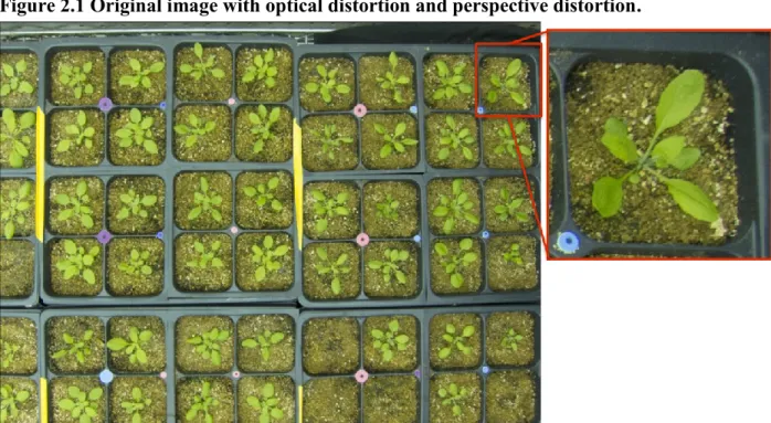
Many previous indoor and field studies used imaging systems (cameras or scanners) and invasive sampling methods (excised plant parts) to extract phenotypic traits (Candela et al. 1999; Pérez-Pérez et al. 2002; Cookson et al. 2007; Bylesjö et al. 2008; Ali et al. 2012; Chitwood et al. 2012). These studies, however, failed to take into account the optical distortion generated by imaging system lenses and the perspective distortion created by the angle of view. True distances and areas cannot be determined from a 2D image if either optical distortion or perspective

distortion are present, and merely facing the imagers straight down does not fix this problem. In particular, if a large number of plants are clustered for imaging, most of the plants will not be at the center of each individual frame. The plants on the corners of each frame will be distorted by the perspective viewing angle of the wide-angle lens (Figure 2.1). The optical distortion and

(31)

perspective distortion of the imaging system must therefore be removed before measuring any geometric quantities from a 2D image.

Therefore, in this chapter, we present a low-cost and fully-automated high-throughput imaging-based phenotyping pipeline suitable for both controlled environments and the field. This pipeline has three advantages compared to other existing pipelines: 1) a low-cost imaging

system, 2) elements of instrument independency, and 3) cross-platform capability. The first advantage is that off-the-shelf, low-cost digital cameras were used as imaging devices instead of other possible remote sensors. This technique allows phenotypic traits (e.g., leaf length, rosette area, diurnal plant nastic movements, and plant vegetation conditions) to be extracted and measured directly from images.

The second advantage of this pipeline is a degree of instrument independency. For example, high-level scripts were used to interface with camera-manufacturer–supplied image processing software. Because many camera manufacturers provide similar tools, exchanging cameras becomes mainly a matter of altering the interface scripts.

The third advantage is cross-platform capability. Although the image data acquisition and data transfer methods may vary in different applications, the pipeline has a generic structure so that it can be deployed on different phenotyping platforms in multiple environments with minimal modification. Specifically, the pipeline was deployed on two different imaging platforms: a stationary growth chamber platform and a movable field platform. The novel,

generic features enabling the pipeline to operate in these very different environments are outlined next.

In particular, the pipeline extracts plant phenotypic traits by: 1) removing image optical distortion and perspective distortion, and 2) applying mathematical algorithms to analyze rosette

(32)

parameters (e.g., rosette center, leaf tips) for total leaf expansion and 2D rosette area

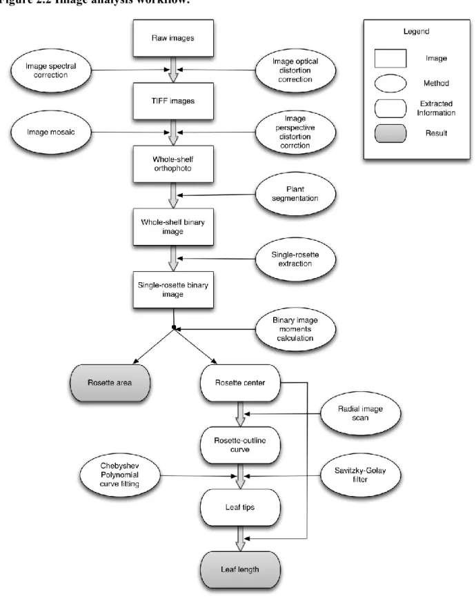
measurements. The workflow for image analysis and extracting rosette parameters from 2D images is shown in Figure 2.2.

Materials and methods

Imaging platform

Indoor imaging platform

The pipeline development was part of a growth chamber experiment conducted at University of California, Davis (UC-Davis) for studying the shade-avoidance response of an Arabidopsis NAM population. A total of 108 Canon Powershot S95 cameras were mounted facing straight down on six shelves—three shelves for simulating sun and three shelves for shade (Figure 2.3A and B). On each shelf, 18 cameras were mounted in a 2-row stationary camera frame 0.4-m height above the shelf surface. Each shelf held 24 (three rows of eight) 4-by-4 pot flats within a 0.80-by-2.13-m area.

Each camera was assigned a three-digit ID comprised of shelf number (1–6), row number (1–2), and camera position (1–9), in that order. Figure 2.3C is one individual image showing the field-of-view (FOV) of each camera and the color dot systems for tracking plant rotation. (The color-dot system is described below in the section on indoor genotype assignment.)

All of the cameras were set on manual focus, manual exposure mode (F7.1, 1/25 s, auto white balance), and a 28-mm (35-mm equivalent) focal length. A modified intervalometer script and the Canon Hack Development Kit (CHDK) firmware were installed on all of the cameras to trigger them simultaneously at the start of each hour. In order to prevent cameras from

(33)

image was taken. All of the images were saved as Canon CR2 RAW format for preserving the maximal amount of geometric, spectral, and camera information.

Field imaging platform

The same genotypes of Arabidopsis used in the chamber were also planted outdoors at the University of Wyoming (UWY) Plant Science Station in Laramie. Plants were grown for a few days in biodegradable pots in the greenhouse and then transplanted to the field in a

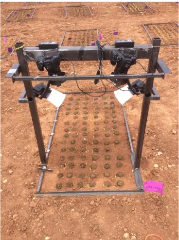
randomized block design. They were placed in a 10-cm grid with 14 rows and 6 columns. Two Canon EOS REBEL T3i DSLR cameras with Canon EF 20mm f/2.8 wide-angle lens were mounted on a moveable camera frame at a 95-cm height above the ground (Figure 2.4). Instead of facing straight down as in the chamber pipeline design, both cameras were mounted angled slightly towards each other to maximize the overlap area of their respective FOV.

For stability and repeatability, the camera mount was placed on a metal frame

surrounding each plot. The inner frame dimensions were 153.0 cm by 73.6 cm. To image the whole plot, the camera mount was first moved to six fixed positions in sequence and pictures were taken. These six pairs did not fully capture all plants, but, because the cameras were on one side of the mount, a seventh position would only have seen the ground outside the plot.

Therefore, the camera mount was turned 180 degrees and a final, seventh pair of pictures was taken.

Two Canon flashes with diffusers were attached on opposite sides of the camera mount. These served to limit the influence of the ambient light changes during the exposure interval and minimize camera mount shadows. Each flash was camera-controlled through an extension cable. Both cameras were set on manual focus, manual exposure mode (F9, 1/200 s, auto white

(34)

Image storing, management, and transfer

Indoor image storing, management, and transfer

All cameras were connected to a local data server at UC-Davis via USB cables for transferring images automatically. A Perl script written by Michael Covington renamed the hourly image files using the combination of the imaging date, time, and camera ID. Nighttime images were deleted and daytime (5:00 am to 8:00 pm) images were stored in the server.

Although all of the 108 cameras were mounted in landscape orientation, the built-in auto rotation function of the cameras would sometimes rotate images to portrait orientation, creating problems in subsequent steps. To fix this, ExifTool (http://www.sno.phy.queensu.ca/~phil/exiftool/), a Perl-based program, was integrated into the pipeline to automatically rotate any RAW images found to be in portrait orientation. Each night, the pre-processed RAW images were transferred to a data store operated by the iPlant and, from there, to a server at KSU. Once the images reached the KSU server, they were organized into different subdirectories based on the imaging date, time, and shelf number. This set of transfers resulted in three redundant copies of the images being maintained at UC-Davis, iPlant, and KSU.

Field image storing, management, and transfer

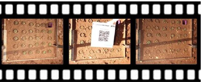
For field image storing and transfer, images were first downloaded from the cameras onto a local computer at UW and then transferred to the data server at KSU via iPlant. Whereas the indoor system used camera ID’s and dates to organize the images, QR codes containing block and plot numbers were employed in the field (Figure 2.5). The QR-code images were first automatically recognized within the stream of images by computing a color histogram and looking for a large number of white pixels. The images containing QR codes were converted to binary using a threshold that removed shadows, then ZBar (http://zbar.sourceforge.net/), a

(35)

freeware QR coder reader integrated into the pipeline, extracted the block number and plot number. This data was used to group the subsequent images into a directory named by image date, block, and plot information.

Missing camera detection mechanism of indoor imaging pipeline During the imaging period, occasionally some cameras would accidently turn off, possibly due to unstable CHDK firmware. If not immediately detected and corrected, gaps in phenotypic data would result. Therefore, we included in the pipeline a mechanism for detecting missing cameras based on tracking the cameras’ IDs in the image names. When missing camera IDs were detected, the pipeline automatically sent an email reporting the problem so it could be manually fixed.

Pipeline control

Agisoft Photoscan Pro (Photoscan), one of the programs to be described below, includes a Python scripting-capable application program interface (API) whose intent is to allow users to automate its capabilities. This was exploited to control all pipeline functions, including, in some cases, the control of programs completely external to Photoscan. The following sections describe all functions used in the processing pipeline, all of which were completely automated within the Photoscan Python API.

Image pre-processing

There were two corrections performed during the image pre-processing section for the images: image color correction and image optical distortion correction. The Canon Digital Photo Professional (DPP) program was used for color correction, optical distortion correction, and TIFF conversion.

(36)

Image color correction

Due to illumination variations across the shelf, the camera color responses differed slightly. For better plant segmentation process in the following step, the color of the RAW images was corrected by the white balance correction function of the DPP program. The spectral-lossless RAW file format was chosen despite its memory requirements to make this possible. Wide-angle lenses are also susceptible to vignetting effects where image brightness is reduced at the periphery. This can complicate color segmentation but was corrected during this process. A customized color-grid poster was photographed to verify the image color correction at the end of the process.

Image optical distortion correction

Few of the previous image-base phenotyping studies have considered lens distortion when extracting leaf parameters (length, width, and area). Due to the geometric distortion caused by lens optics, those leaf measurements have reduced accuracy for plants not at the center of each image. Using the RAW file format also allowed us to use manufacturer-provided lens profile data to correct the geometric distortion of each plant—another function built into DPP. After image color correction and optical distortion correction, TIFF image files were exported. The color-grid poster was also used for verifying the image optical distortion correction.

DPP automation

A design drawback of DPP is that it assumes a human will be using it to correct a small number of images. Thus, it lacks any automation capabilities. Therefore, AutoIt

(https://www.autoitscript.com/site/autoit/), a BASIC-like scripting language, was used to

automate the DPP graphical user interface (GUI). This language simulates user mouse clicks and text entries. While this may seem cumbersome, it is actually a major advantage of the pipeline.

(37)

Aside from the Perl script described, the AutoIt script is the only element of the pipeline that would have to be altered if a different brand of camera and manufacturer-provided image correction software were adopted.

Orthophoto generation

The final type of correction removed image perspective distortion. This was done by generating orthophotos, which are synthetic images produced as if each pixel is being viewed straight down. Thus, orthophotos permit geometric quantities such as 2D distances and areas to be measured with perspective effects removed. The Agisoft Photoscan Pro (Photoscan) program (http://www.agisoft.com) performed this step using the TIFF images output from DPP. This was done in nine-image subsets, each of which covered one half-shelf. (The original intent was to do full shelves but it was discovered after plants were added to the chamber that the vertical camera spacing did not permit this—a design flaw to be avoided in the future.) The program converted each set to an orthophoto. However, in the process of implementing this step, a subtle difference between the chamber and the field was uncovered that affected exactly how this should be done. This is described in the following two subsections.

Indoor environment image rendering method

Photoscan has four alternative rendering options for producing orthophotos: Mosaic, Average, Max Intensity, and Min Intensity. These govern the coloring method used to merge corresponding pixels from different images into the orthophoto. It was discovered that a wrong choice could have side effects for the small fraction of leaves that happened to have very different orientations with respect to different cameras. Specifically, the leaves would appear to be ghost-like double exposures. This was corrected by choosing the Mosaic method that favored

(38)

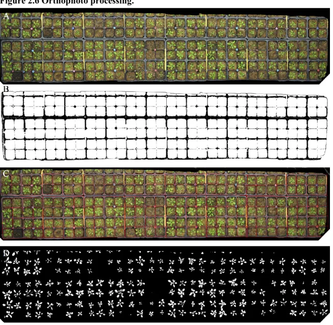
the camera whose view of ghost leaves was most vertical. An example orthophoto is shown as Figure 2.6A.

Field image rendering method

When used in the field, however, the Mosaic rendering method left pronounced shadows in the orthophoto that complicated subsequent processing steps. This was resolved by using the Average rendering method. This produces a more uniform orthophoto because areas that are shadowed by the camera mount in one image will often not be shadowed in others. Because it blends pixels, the Averaging method reduces shadow contrast.

To summarize the pipeline control description, Python scripts written and executed within Photoscan first invoke AutoIt to run a script in that language simulating user keystrokes and mouse clicks instructing DPP to remove lens and color distortion and produce TIFF

formatted images. Once AutoIt processing is finished, the Python script then initiates Photoscan operations that produce the orthophoto. The same script then continues, executing the operations described in the following sections.

Image segmentation

Pot segmentation

In order to extract individual plants from each chamber orthophoto, the first step is to apply image segmentation to identify the pots. This was done using the following equation:

𝑃𝑜𝑡 = 𝑏𝑤(𝐵𝑙𝑢𝑒 − 𝑅𝑒𝑑),

where Blue is the pixel brightness value of the image blue channel, Red is the pixel brightness value of the image red channel, and bw() is the Otsu threshold method (Otsu 1975) for binary image transformation. Due to the slight illumination variation across each shelf, some of the pot

(39)

edges could not be detected. The probabilistic Hough Transformation (Duda and Hart 1972) was implemented in Python to identify the line segments and fill in the missing pot edges (Figure 2.6B). A 4-by-4 grid was generated for each flat based on the known dimensions of the pots and flats (Figure 2.6C).

Plant segmentation

Plant segmentation, the process of isolating the plants from other unwanted image features like soil, pots, or other items, is the next process applied to each orthophoto. The well-controlled illumination sources and image color corrections in the previous step allowed us to use a simple vegetation index for quick plant segmentation. The vegetation index used for this study computes the difference between the green and red channels and uses a ratio to normalize it throughout the entire imaging period. This measure, the Normalized Green–Red Difference Index (NGRDI) developed by Hunt et al. (2005), is similar to the well-known Normalized Difference Vegetation Index (NDVI). However, NDRDI is more useful to distinguish healthy vegetation from background in cameras like ours that have not been modified to be infrared-sensitive. The Otsu threshold method was then applied for transforming grayscale NGRDI images to a binary form in which the plant pixels are white and all non-plant pixels are black. The NDRDI equation in this study is as follows:

𝑃𝑙𝑎𝑛𝑡 = 𝑏𝑤 (𝐺𝑟𝑒𝑒𝑛 − 𝑅𝑒𝑑 𝐺𝑟𝑒𝑒𝑛 + 𝑅𝑒𝑑),

where Green is the pixel brightness value of the image green channel, Red is the pixel brightness value of the image red channel, and bw() is the Otsu threshold method for binary image

transformation. The processed binary orthophoto is shown as Figure 2.6D. The NGRDI equation was implemented in Python and the Otsu threshold was from the Open Source Computer Vision Library (OpenCV; http://opencv.org/).

(40)

Plant genotype assignment

Indoor pipeline genotype assignment

Although growth chambers are well controlled, there are still temperature and lighting gradients that can affect plant growth and development. It is therefore common practice in Arabidopsis experiments to randomly reshuffle flats of pots every two to three days. Flat

movements are recorded in spreadsheet form, but, to provide redundancy within the image data, a system using three-color dot combinations on each flat was developed. A color-dot detection and decoding routine was integrated into the processing pipeline for automatically tracking pots so that the proper genotypes of each plant could be paired with the ultimate measured

phenotypes.

Field pipeline genotype assignment

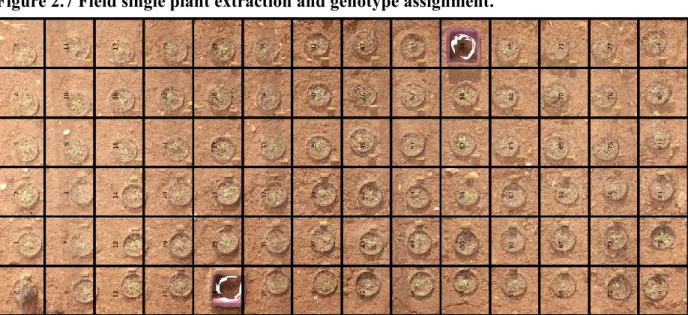
Because all of the plants were placed with a 14-by-6 planting grid in each plot of the field study, a Python routine was integrated in the pipeline to generate a 14-by-6 grid on each plot orthophoto for extracting plants. However, due to some irregularities of planting grid placement in each plot, each plot orthophoto needed to be cropped first so the grids were generated in appropriate positions (Figure 2.7). As each plant was extracted, plant position and QR-code data on block and plot number was used to rename each single-rosette image. This information was paired with the genotype metadata collected when plant locations were assigned.

Phenotypic traits extraction

Leaf length and total leaf expansion calculation

The key step in measuring leaf length is the detection of the rosette center and leaf tips on each single-rosette binary image. The contours of each binary image were analyzed first and the

(41)

image moments were then calculated (https://en.wikipedia.org/wiki/Image_moment). The rosette center was estimated using the binary image centroid of all white (i.e., plant) pixels. That is:

(𝑥̅, 𝑦̅) = (𝑀10 𝑀₀₀,

𝑀₀₁ 𝑀₀₀),

where 𝑥̅ and 𝑦̅ are the coordinates of the binary image centroid and M are image moments. Using the calculated rosette center as the origin, a radial scan was executed on the binary image to yield a curve representing the traced rosette outline in a 2D plot. The leaf tips, the points most distant from the plant center, should be the peaks of the curve just described. However, at first it was challenging to find accurate peak locations due to the rough edges of plant leaves. This was even more complicated when parts of the leaves appeared to be missing due to damage or segmentation faults. Therefore, the rosette-outline curve was first smoothed using Savitzky–Golay filter (Savitzky and Golay 1964) so small, erroneous maxima could be removed. The next step was to fit a Chebyshev polynomial (Tchebychev, 1853) to the smoothed rosette-outline curve. Putative peaks were then located by calculating the roots (i.e., zeros) of the first derivative of the Chebyshev polynomial curve. Unfortunately, this procedure still yielded false leaf tip positions sometimes.

Therefore, as a second step, the peak widths were analyzed using the x coordinates of the rosette-outline curve to find the minimum peak width, which was used as the length of a moving window centered at each detected curve peak. Within this moving window, the maximum of the fitted rosette-outline curve and the maximum of the original rosette-outline curve were

compared. The true peak locations were recovered if the maximum of the original rosette-outline curve was higher. The pixel coordinates of the leaf tips were calculated based on the curve peak locations. The length of each leaf was measured as the distance from the rosette center to the leaf tip. The total leaf expansion of each plant is the sum of all of the leaf lengths.

(42)

Rosette area calculation

The rosette area in each single-rosette binary image can be simply calculated by computing the total number of white pixels in each single-rosette binary image.

Statistical modeling

Chitwood et al. (2012) manipulated far-red light to induce changes in leaf length as an index of the shade-avoidance response. This study demonstrated a linear relationship between total leaf length and square root of the total leaf area. To test the relationship between total leaf expansion and rosette area using our workflow, we implemented the power law function to fit the phenotype data with the following equation:

𝑇𝑜𝑡𝑎𝑙 𝐿𝑒𝑎𝑓 𝐸𝑥𝑝𝑎𝑛𝑠𝑖𝑜𝑛 = 𝑎 ∗ 𝑅𝑜𝑠𝑒𝑡𝑡𝑒 𝐴𝑟𝑒𝑎𝑏,

where a and b are parameters that determine the trajectory and shape of the power law function, respectively.

The parameters a and b were estimated using the Levenberg-Marquardt non-linear least square method. Bootstrap resampling was used to calculate 95% confidence intervals (CI) based on 10000 simulations. The power law function and the least square estimation were implemented using Python Scipy package.

Indoor pipeline data analysis

Data for total leaf expansion and rosette area measured on four different dates during a 10-day growth period were used for the analysis. The first set of data was collected the eighth day after plant emergence, followed by three subsequent datasets at two-day intervals. The time points of this test were selected so that: 1) the plants were big enough to distinguish individual leaves from the start, 2) the final image had a large rosette, and 3) leaf overlap areas between

(43)

adjacent plants were minimal. All of the images from the indoor pipeline were taken at 6:00 am to minimize any possible ambient influences.

Field pipeline data analysis

The same genotypes tested in the indoor environment were also tested in the field experiment. Data from six different days were used to fit the same relationship. They were selected from an 18-day period in which Day 1 was the third day after plants were transplanted in the field. Five subsequent dates, each three to four days apart, followed. (The dates of field image data collection were dependent on weather conditions.)

Results and discussion

Indoor imaging pipeline throughput capability

Because there was a certain amount of unavoidable manual work during image acquisition in the field, the completely-automated indoor pipeline was used to evaluate the throughput capability of the phenotyping pipeline.

Orthophoto generation, which initially required 38 CPU-minutes per half-shelf, was the most time-consuming process in the entire pipeline. By implementing High Performance Computing (HPC) routines using OpenCL and AMD GPUs in the pipeline, this processing time was reduced to 25 minutes per half-shelf orthophoto. These HPC routines were also utilized in other steps. It took approximately 6–8 minutes to detect pots and decode the color dots for genotype assignment, then two minutes for extracting phenotypic trait data (e.g., total leaf expansion, rosette area). Therefore, the total runtime of the entire processing pipeline was 35 minutes maximum for each half-shelf.

The second method for improving pipeline throughput was to use distributed parallel computing routines to spread the processing tasks across a small computing cluster. Two split

(44)

half-shelf orthophotos from each shelf were processed by two nodes simultaneously. For the chamber application, there were 24 4-by-4 pot flats on each of the six shelves, which made 2,304 plants photographed hourly. Because imaging was conducted for 16 hours per day, a total of 36,864 single-plant pictures were obtained each day. Each cluster node processed 192 plant images in 35 minutes, equating to at least five plants per minute. Therefore, the runtime for processing 16 hours of single-rosette images on the six-node cluster was 11.2 hours. The capabilities of the chamber processing pipeline are shown in Table 2.1.

This pipeline was fast because all 108 cameras took images for six shelves

simultaneously. The times for image storing, management, and transfer have not been included in this analysis because of variations in local network and internet speeds. In the future, when the processing pipeline is executed on a local computer cluster at UC-Davis for minimizing data transfer time, all 2,304 plants can be screened within an hour.

Image analysis

Image optical distortion and color correction

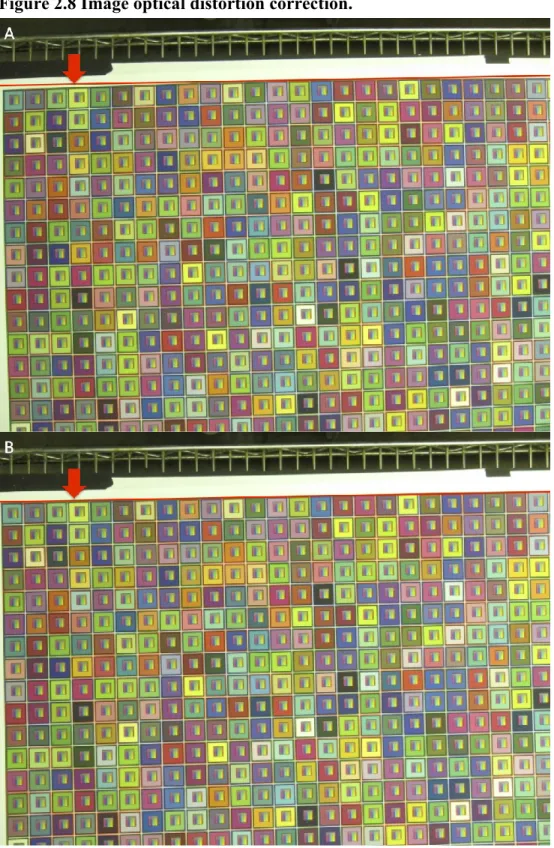
The 28-mm (35-mm equivalent) focal length caused the optical distortion to be much more severe on the image edges than on the image center. Figure 2.8A shows the color-grid image before optical distortion removal. The red reference line was drawn on the image to illustrate the curvature of the color grids caused by the optical distortion. Using Canon DPP to remove optical distortion was accurate and efficient because of the manufacturer’s lens profile database. Figure 2.8B shows that the curvature of the edges of color grids was removed after the optical distortion correction. The red reference line matched the edge of the color grid.

Due to variations in shelf illumination and camera firmware differences, the original images were greener than the original RGB values of color grids. After comparing different

(45)

image color correction packages, the Canon DPP software provided reasonably accurate color correction using the white balance function provided by the camera manufacturer. After color correction, the green tone was removed and the photographed RGB values were very close to the original (Figure 2.9).

Image perspective distortion correction

Figure 2.10 (A–B) shows two plants at the corner of the individual frame. The effects of perspective are clear because a great deal of pot wall can be seen compared to plants at the image centers, where much less wall is visible. Due to this issue, direct measurements from the image centers and corners are not comparable; Figure 2.10 (C–D) shows that after re-projecting each pixel vertically. The sidewalls of the pots were largely corrected and only a small portion of the pots’ sidewalls were visible compared to the uncorrected images. Moreover, the red-box– highlighted leaves showed more leaf area in the corrected image for both of the plants when the leaves were not entirely flat. The two pots shown in Figure 2.10 are from the most extreme corners of the shelf, so the small portions of visible sidewalls are inevitable. For most of the pots, the sidewalls were well corrected.

Moreover, the blue-box–highlighted leaves show that leaf positions were also corrected. For plant 1 (Figure 2.10A), the two leaves in the blue box showed a side-by-side position, but in reality, the smaller leaf was under the big leaf, as the corrected image shows (Figure 2.10C). For plant 2, the two leaves highlighted by blue boxes overlapped in the uncorrected image but distinguished clearly after correction (Figure 2.10B and 2.10D). Although smaller leaves could not be counted when covered by bigger leaves, the perspective-distortion–corrected images will provide more accurate leaf length and rosette area measurements, which are more critical when studying leaf shade-avoidance responses.

(46)

Rendering methods for indoor and field orthophoto

Most previous studies did not use orthophotos for extracting phenotypic traits from 2D images and therefore did not have occasion to compare rendering methods. In the chamber, each plant appeared in two views, one necessarily more oblique than the other. In a small number of cases, the leaf angles were sufficiently extreme that, depending on how the orthophoto was rendered, a double image of the leaf would result. Figure 2.11 illustrates the double image problem and how it was resolved using the Mosaic method, which colors the orthophoto using the image pixels that resolve as being closest in 3D space.

The red-box–highlighted leaves in Figure 2.11A and B were photographed with different viewing angles by adjacent cameras 514 and 515. In this instance, a small leaf was covered by a bigger leaf. Camera 515 photographed them at an oblique angle so both leaves were visible to this camera but not to Camera 514. Because of this, under the Average rendering method, which blends corresponding pixel colors from both images, the highlighted leaf appears twice in the orthophoto (Figure 2.11C). This defect would subsequently confuse the leaf tip detection algorithm. However, in Figure 2.11D, when the Mosaic rendering method was used, the plant outline was not confusing and the “double-leaf” issue was solved.

There are actually three defects in Figure 2.11 which need to be discussed: one is partial overlap (top red box), one is different viewing angle (middle red box), and the last is complete overlap (bottom red box). With the Average method, all three create spurious leaf tips due to differences in the “opacity” of the double images. However, the Mosaic method fixes this issue at the cost of occasionally losing an entire leaf (bottom red box).

On the other hand, in the field environment, the two cameras were relatively far away from the plants, so the viewing-angle issue was not as pronounced as in the chamber. Instead, the

(47)

major problem affecting rendering was the strong ambient illumination by sunlight, which cast constantly-changing shadows of the camera mounts into the plots. Originally, it was thought that the flashes could be used to completely eliminate shadows. Unfortunately, this required their most powerful settings, which saturated image brightness. Therefore, a lower setting was used in combination with the Average rendering method to improve the consistency of the brightness of the orthophoto. Figure 2.12A shows pronounced camera mount shadows when the Mosaic rendering method was used. Subsequent image segmenting by color analysis was not able to achieve equal results at identifying plants under shadowed and non-shadowed conditions. However, in Figure 2.12B, the orthophoto produced by the Average rendering method shows more uniform brightness throughout the entire plot. These images could be successfully segmented even though the shadows were not completely eliminated.

Field QR codes imaging and processing

QR codes provided a very efficient way to store plot metadata and organize plot images. Initially, the ground-level field pipeline could successfully recognize all of the QR-code images among other field images by analyzing the histograms of the images, but there were some failed attempts when the ZBar reader tried to decode the QR codes. The failed attempts occurred when the shadow of the camera mount fell on the QR codes. To solve this issue, the brightness and contrast of all of the recognized QR-code images were first increased to minimize the shadow, then the adjusted images were thresholded to a shadow-free binary image. With this

improvement, all of the QR codes were successfully decoded and the plot metadata was accurately extracted.

(48)

Accurate leaf tip detection is critical to measuring leaf length and total leaf length expansion. Initially, however, many false leaf tips were detected, due to small irregularities on the original rosette-outline curve (Figure 2.13). As Figure 2.14 shows, the estimated peak locations were shifted from the original rosette-outline curve peak locations, and peak heights were lowered due to smoothing after the Savitzky–Golay filter and the Chebyshev Polynomial curve fitting. However, after the second iteration of the leaf tip detection, most of the peak locations from the first iteration were shifted back to the original radial-scan-yield curve peak locations, true peak locations were recovered, and many false peaks were eliminated. These optimization operations provide much more accurate rosette-outline peaks for positioning the true leaf tips on the single-rosette binary image. This method was especially accurate and efficient for finding the leaf tips when the leaves were damaged, as in the example in Figure 2.14.

Relationship between rosette area and total leaf expansion

Relationship for indoor pipeline

The estimated parameter b of the power law function from Day 1 to Day 4 is 0.836 (Figure 2.15A), 0.753 (Figure 2.15B), 0.750 (Figure 2.15C), and 0.636 (Figure 2.15D),

respectively, indicating a change in shape from near-linearity to a more curved relationship. The range of possible estimates for parameters a and b obtained from 10000 bootstrap simulations is shown in Figure 2.16. The histograms shows the frequency of estimate for a and b in 10 bins. The mean, median, and mode for a and b, respectively, are very close to the original estimate from the least squares fit. The analyses of the parameter distributions and the bootstrap 95% confidence intervals are shown in Table 2.2.

(49)

Because the confidence limits for Days 1 and 4 do not overlap, it can be said that the exponent of the power law decreases with time while the slope factor increases, although there is considerable uncertainty about the values of parameter a. However, the range of values for b is within the reasonable expectations of being not greater than 1 and not less than 0.5. These values are consistent with the idea young leaves mainly grow by elongation. However, in later

developmental stages, total leaf expansion slows relative to leaf-width growth increases, which become the main contributor to increasing rosette area. Chitwood et al. (2012) reported a linear relationship between total leaf length and square root of the total leaf area (i.e., b=0.5) for tomato leaves at a late developmental stage. This result is very similar to our finding of b=0.636 during late development.

This dynamic relationship between total leaf expansion and rosette area has not been reported previously, quite possibly because destructive sampling made it impossible to collect time-series data from the same plant during growth. Our non-invasive imaging method, however, can be used to track the time-series development pattern for single plants in a mapping

population.

Relationship for field pipeline

The estimated parameters a and b and the power law curves for Days 1 to 6 in the field are shown in Table 2.3 and Figure 2.17A-F, respectively. The b values also followed a

descending trend over time. Figure 2.18 shows the analyses of the parameter distributions and the bootstrap 95% confidence intervals. This result follows what is seen in the chamber; that is, b is close to 1 at the beginning of the growth period but decreases over time. As above, the