Published by: IEEE
URL:
http://dx.doi.org/10.1109/ACCESS.2018.2880416
<http://dx.doi.org/10.1109/ACCESS.2018.2880416>
This version was downloaded from Northumbria Research Link:
http://nrl.northumbria.ac.uk/36965/
Northumbria University has developed Northumbria Research Link (NRL) to enable users to
access the University’s research output. Copyright © and moral rights for items on NRL are
retained by the individual author(s) and/or other copyright owners. Single copies of full items
can be reproduced, displayed or performed, and given to third parties in any format or
medium for personal research or study, educational, or not-for-profit purposes without prior
permission or charge, provided the authors, title and full bibliographic details are given, as
well as a hyperlink and/or URL to the original metadata page. The content must not be
changed in any way. Full items must not be sold commercially in any format or medium
without formal permission of the copyright holder. The full policy is available online:
http://nrl.northumbria.ac.uk/policies.html
This document may differ from the final, published version of the research and has been
made available online in accordance with publisher policies. To read and/or cite from the
published version of the research, please visit the publisher’s website (a subscription may be
required.)
Date of publication xxxx 00, 0000, date of current version xxxx 00, 0000.
Digital Object Identifier
Evolving Image Classification
Architectures with Enhanced Particle
Swarm Optimisation
BEN FIELDING, AND LI ZHANG, (Member, IEEE)
Department of Computer and Information Sciences, Faculty of Engineering and Environment, Northumbria University, Newcastle upon Tyne, UK, NE1 8ST Email: {ben.fielding; li.zhang}@northumbria.ac.uk
Corresponding author: Li Zhang (email: [email protected]).
The authors would like to thank RPPtv Ltd and Northumbria University for their funding support towards this work.
ABSTRACT Convolutional Neural Networks (CNNs) have become the de facto technique for image feature extraction in recent years, however their design and construction remains a complicated task. As more developments are made in progressing the internal components of CNNs, the task of assembling them effectively from core components becomes even more arduous. To overcome these barriers, we propose Swarm Optimised Block Architecture (SOBA), combined with an enhanced adaptive Particle Swarm Optimisation (PSO) algorithm for deep CNN model evolution. The enhanced PSO model employs adaptive acceleration coefficients generated using several cosine annealing mechanisms to overcome stagnation. Specifically, we propose a combined training and structure optimisation process for deep CNN model generation, where the proposed PSO model is utilised to explore a bespoke search space defined by a simplified block-based structure. The proposed PSO model not only devises deep networks specifically for image classification, but also builds and pre-trains models for transfer learning tasks. To significantly reduce the hardware and computational cost of the search, the devised CNN model is optimised and trained simultaneously, using a weight sharing mechanism and a final fine-tuning process. Our system compares favourably with related research for optimised deep network generation. It achieves an error rate of 4.78% on the CIFAR-10 image classification task, with 34 hours of combined optimisation and training, and an error rate of 25.42% on the CIFAR-100 image data set in 36 hours. All experiments were performed on a single NVIDIA GTX 1080Ti consumer GPU.
INDEX TERMS Computer Vision, Convolutional Neural Networks, Deep Learning, Evolutionary Com-putation, Image Classification, Particle Swarm Optimisation
I. INTRODUCTION
D
ESPITE being a relatively mature concept, Convolu-tional Neural Networks (CNNs) have proven to be in-credibly effective feature extractors in recent computer vision research. They were originally proposed and proven effective by LeCun et al. [1] in 1989 for classifying handwritten numerical digits from a dataset now commonly known as MNIST, but subsequently fell out of favour for a number of years. Since then, CNNs have experienced a large resur-gence in popularity, particularly for challenging computer vision tasks requiring effective feature extraction. This rise in popularity has been motivated largely by the increases in performance demonstrated by CNNs on challenging tasks such as the ImageNet Large-Scale Visual RecognitionChal-lenge (ILSVRC) [2]. The ILSVRC has been running annual competitions since 2010, backed by the ImageNet dataset which contains over 14 million images with various asso-ciated metadata, organised to follow the paradigms of the popular WordNet dataset [3]. Since 2015, all of the winners, and a majority of the entrants, have each been some variation of a deep CNN, with a newly proposed architecture being the improving factor for a number of the entrants. Often these new architectures are then used by subsequent works in relevant sub-fields by exploiting the pre-trained networks as essentially pre-created feature extractors and using transfer-learning techniques to apply them to the new tasks. Since this widespread adoption of deep convolutional networks as the go-to technique for image feature extraction, it has become
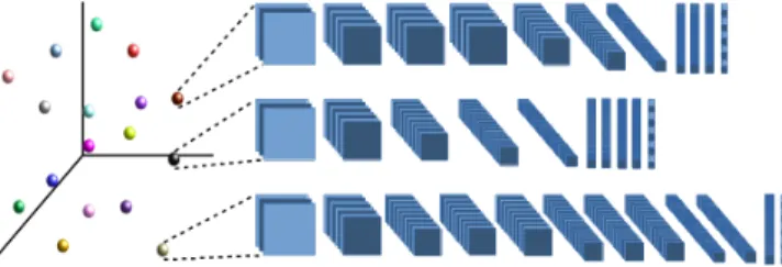
Fig. 1: The proposed Swarm Optimised Block Architecture where each particle represents a full, discrete convolutional architecture for image classification.
necessary for many researchers to integrate these pre-trained networks into their own models, where previously they would have used a hand-designed feature extractor such as SIFT [4] or HOG [5]. Currently, the choice of pre-trained network comes from the few existing, well-known architectures that have been proposed and validated in deep learning literature, but modifying these architectures to better suit a particular task requires deep domain knowledge that is often unavail-able to researchers or end-users in many sub-fields.
In this research, we refer to the specific combination of layers and parameters that make up the structure of a CNN as the ‘architecture’ of the network. This combination of design choices rapidly becomes larger as the intended depth of a net-work increases. The architectures of the netnet-works described above have largely been designed by hand, using expert knowledge in order to tweak parameters and hyperparameters to achieve the best possible results. This has unfortunately resulted in a high barrier-to-entry for the field, as this expert knowledge must be acquired before one can design effective networks. The process can be seen as a sort-of human-led stochastic optimisation, whereby human agents iteratively design and test new architectures, using knowledge gained through previous experiments or from others’ experimental results. When applying to sub-field tasks, transfer learning implementations rely on existing pre-trained models due to the time/hardware constraints, difficulty in designing and training a new model, and the potential pitfalls in this process. This does, however, mean that the pool of available networks is very small, as one must rely solely on the published architectures. Therefore an automatic architecture optimisa-tion process is required to allow these researchers to design architectures specific to the task at hand without needing a deep background knowledge in the area. The process must also be fast and usable on commodity hardware, in order to be available to those who need it the most.
In this work, we propose Swarm Optimised Block Ar-chitecture (SOBA), a system to perform evolutionary deep CNN model generation using an enhanced Particle Swarm Optimisation (PSO) model. The proposed model is able to conduct concurrent architecture optimisation and end-to-end training for the task of image classification. In other words, the proposed method both optimises and trains model archi-tectures at the same time, allowing a ‘one-click’ approach
to creating an effective model from a block-based skeleton architecture. Using this approach, we provide an effective way to optimise the architecture of CNNs for image classi-fication through the formation of the optimisation problem within a constrained search space. We employ a skeleton architecture that is used as a minimal starting point by our optimisation system, which loosely follows the VGG architecture [6]. A modified PSO model with adaptive ac-celeration coefficients is used to perform the evolving deep CNN generation, with parameter sharing used to alleviate the enormous computational cost of fully training and evaluating each new architecture. The newly proposed cosine annealing mechanisms for adaptive search weight generation in the enhanced PSO model enable the search to balance between local exploitation and global exploration to carefully direct the architecture generation around the additional constraints introduced by the parameter sharing strategy. The nature of the search process in combination with the training of the network blocks themselves ensures that each block becomes much more robust, as it is trained and optimised to its best performance level, regardless of the structure of the rest of the network. Specifically, each block will be trained using backpropagation independent of the specific configurations of the other layers, with the weights shared between differ-ent model configurations. This strategy is contrary to hand-designed models which are wholly trained with the same model configuration. Fig.1 represents the proposed Swarm Optimised Block Architecture (SOBA) model.
The research contributions are as follows:
1) We formulate the optimisation problem within a con-strained search space through the creation of a bespoke objective function.
2) We employ a continual training method using a weight lookup table to alleviate the enormous computational cost of fully training and evaluating each new architec-ture.
3) An enhanced PSO model is proposed to perform the minimisation of our objective function with acceleration coefficients determined by a shifted cosine function to address the added constraints from our continual train-ing method.
4) We apply a combined optimisation and training strategy to provide single-run, end-to-end optimisation with a final fine-tuning step.
5) Evaluated on the CIFAR-10 and CIFAR-100 image datasets, the proposed model shows superior classifica-tion performance on consumer hardware in reasonable time, over other related methods reported in the litera-ture.
The proposed SOBA model allows for fast, effective de-sign & training of simple VGG-style image classification models up to a high level of accuracy through stochastic exploration of a constrained euclidean search space, inspired by the simple and popular VGG architecture model. SOBA is designed and tested using consumer-level hardware with
reasonable runtimes, providing an accessible method of ar-chitecture optimisation with huge potential for other complex computer vision tasks.
The rest of this paper is organised as follows. We discuss the background theory and related work in Section II, and present the proposed SOBA optimisation model for evolving deep CNN generation with adaptive PSO and weight sharing in Section III. We then provide system evaluation and exper-imental results in Section IV. Finally, we provide concluding remarks and discuss further directions in Section V.
II. BACKGROUND & RELATED WORK A. ARCHITECTURE OPTIMISATION
Evidenced by recent research [7], [6], [8], [9], CNNs have become exceedingly popular for solving computer vision problems owing to their ability to learn task-specific filters to extract the key information in an image. CNNs are usually comprised of multiple layers of computation that function together to form a network. When designing a CNN for classification, the typical goal is to embed the information found in the image into a fixed length vector, which can then be passed through fully-connected (linear) layers, or even another classifier, to finally output class probabilities. This is performed by cascading layers of convolutional operations with learned filters. There are a number of design and param-eter choices that can be made for each layer, as well as for the connections between the layers. The traditional approach is a purely hierarchical model, where each layer feeds its output feature maps into the next layer sequentially until the final layer is reached. Recent works have, however, explored the possibility of considering the connections between the layers as a Directed Acyclic Graph (DAG), whereby each layer can connect to any number of subsequent layers. This approach is motivated by the success of residual or skip-connections [9], which proved effective at maintaining global features throughout the network by directly passing earlier feature maps to later layers in a hierarchical network. Besides the connections between the layers in the network, each layer itself requires a number of choices to be made pertaining to its parameters and functionality. As previously mentioned, these choices have traditionally been made based on prior knowledge and intuition, with many combinations being thoroughly tested before an optimal architecture is found. There has been a large amount of recent interest in the task of designing architecture search strategies to replace this human-led trial and error process and provide an effective method to automatically design optimal architectures and associated hyper-parameters. As an example, Stanley and Miikulainen [10], [11], [12] explored various methods for automating the process of designing neural network architec-tures. Their method, called NeuroEvolution of Augmenting Topologies (NEAT), took the form of a Genetic Algorithm (GA) which could ‘grow’ architectures from a simple start-ing point. Stanley et al. [13] also explored trainstart-ing neural networks via similar evolutionary methods, although this has thus far not proved to outperform backpropagation. There has
been some recent work to extend the NEAT methodology to build deep learning architectures, as the size and complexity of CNN models present further challenges [14], [15], [16], [17]. More recently there have been a number of experiments using reinforcement learning (RL) for automated architecture design [18], [19], [20], [21], [22], although these techniques have very recently been surpassed by relatively more simple evolutionary methods [23], [24], [25], [26].
In [25], Real et al. demonstrate evolution of image clas-sifiers using relatively few constraints. They inherit weights between evolutionary generations for more effective training with less wasted processing time for re-training layers of the same shape/depth in the architecture. Their model uses a form of tournament selectionwhereby an initial population of models is trained, then individual pairs are compared and the weaker of the pair is terminated. On the contrary, the fitter solution of the pair is selected for reproduction to yield an offspring solution via a mutation operation. This offspring model is then trained and evaluated and becomes a member of the overall population and the above process is repeated. Mutations are chosen from a population of eleven hand-picked operations (such as Insert-convolution, Alter-learning-rate, and Alter-filter-size) intended to mimic the steps a human would take when attempting to improve the architecture. Their work could also be extended to yield “hybrid evolutionary–hand-design methods” in the future.
Brock et al. [27] train a ‘hypernetwork’ model to gener-ate weights for a given architecture, in order to effectively evaluate an architecture’s validation performance. They can then sample architectures to obtain validation performance estimates using the weights generated by the hypernetwork. Once a number of architectures are generated and sampled, they take the architecture with the best estimated validation performance and fully train it in the usual way, in order to test its performance on the test set.
Zoph and Le [19] use a recurrent neural network (RNN) as a controller network to generate potential network archi-tectures. These architectures are trained for a large num-ber of epochs and then evaluated on a validation set to determine a score for the child architecture. The controller architecture is trained using policy gradients, particularly the REINFORCE algorithm [28]. Owing to the enormous cost of training for evaluating each child architecture, an asyn-chronous, distributed training process is used whereby many child architectures are trained concurrently using multiple workers. This approach is common for current architecture optimisation works, although it does require huge resources not commonly available to research teams.
Negrino and Gordon [29] propose a method that allows researchers to describe search spaces, which can then be ef-fectively explored using a tree-search strategy. They demon-strate the effectiveness of Monte Carlo tree search (MCTS) and sequential model-based optimisation (SMBO) over ran-dom search when traversing their defined search spaces.
Baker et al. [18] use Q-Learning to maximise the overall expected reward by modelling architecture optimisation as
a Markov Decision Process (MDP). Their agent iteratively selects layers to add to the architecture, until it reaches a stop-state. Initially the agent is allowed to sample architectures with a random walk, giving the opportunity to explore the search space before targeted optimisation. They allow the agent to continue this random behaviour to a certain extent, until the end of the process, producing a number of different models which can then be evaluated as an ensemble in order to improve final performance.
Besides the above, Real et al. [30] perform the first con-trolled comparison of reinforcement learning and evolution-ary methods for architecture optimisation and found that “regularized evolution consistently produces models with similar or higher accuracy across a variety of contexts with-out need for re-tuning parameters”.
Wang et al. [31] proposed a method using the PSO model to optimise architecture, with an embedding scheme derived from IP address allocation. Unfortunately, their proposed system was unable to effectively deal with the issue of function-evaluation cost, whereby each particle evaluation is prohibitively time and resource expensive when performed as a full training-evaluation process. They implemented early evaluation, where each individual was partially trained on the training dataset and then evaluated on the validation set for each fitness function evaluation. This is effective at reducing the time required for each function evaluation, but results in unreliable fitness scores due to the fact that each architecture has not been trained to its full extent when evaluating and it is impossible to know when its performance will plateau. Their work thus showed limited capabilities to be tested on any datasets other than the decidedly small MNIST dataset. Their system performed favourably in comparison with the other methods, although it is notable that they did not compare against any key deep learning architectures, or indeed any systems proposed in recent years.
The drawbacks of the vast majority of these works are that they focus on the optimisation of the architecture as a distinct search problem, and separate it from the actual training of the model for the specific task. This results in these methods having two distinct steps, i.e. resource-heavy optimisation, followed by lengthy training in order to generate the model with the most promising performance. This motivates the proposed work in this research to jointly optimise and train an identified deep learning model to enhance both system performance and computational efficiency. The proposed SOBA optimisation model also employs a weight sharing mechanism to overcome the function-evaluation cost issue encountered by [31] and discussed above.
B. PARTICLE SWARM OPTIMISATION
Particle Swarm Optimisation (PSO) [32] is a stochastic op-timisation technique that relies on a population X of m individuals, each with a specific position in the search space defined by a fixed-length vector Rn. Each position in the
search space represents a distinct set of parameters to an objective function f. The fitness of an individual particle
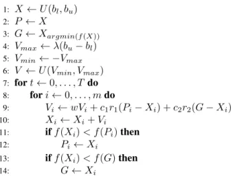
1: X ←U(bl, bu) 2: P ←X 3: G←Xargmin(f(X)) 4: Vmax←λ(bu−bl) 5: Vmin← −Vmax 6: V ←U(Vmin, Vmax) 7: fort←0, . . . , T do 8: fori←0, . . . , mdo 9: Vi ←wVi+c1r1(Pi−Xi) +c2r2(G−Xi) 10: Xi←Xi+Vi 11: iff(Xi)< f(Pi)then 12: Pi←Xi 13: iff(Xi)< f(G)then 14: G←Xi
Fig. 2: The original PSO algorithm
represents the result of evaluating the objective function f with the position of the particle as parameters. The goal of PSO is to minimise or maximise the objective evaluation by finding the best overall particle position argminxf(x) orargmaxxf(x). The individual particles in the population are initialised with random positions in the search space, usually by drawing their values from a uniform distribution U, bounded by defined upper (bu) and lower (bl) bounds. The particles are then iteratively evaluated and conduct the search process by following personal and global best solutions in order to attain global optimality. Specifically, as the particles are moved around the search space, the best positions found so far, along with their fitness scores, are stored for each individual particle. These are referred to as the ‘local best’ solutions. The best solution of the overall swarm is referred to as the ‘global best’ solution and indicates the best set of parameters that the algorithm has as-yet found for the objective function. (1) & (2) denote the velocity and position updating operations for each particle respectively.
Vit=wVit−1+c1r1(Pi−Xit−1) +c2r2(Pg−Xit−1) (1) Xit=Xit−1+Vit (2) where c1 and c2 denote acceleration coefficients, and r1 andr2 are random vectors drawn fromU(0,1)to introduce stochasticity.PiandPgrepresent the personal and global best solutions respectively, with w as the inertia weight. Xit−1 andVit−1represent the position and velocity of the particlei from the previous (t−1) iteration, respectively. The process is repeated over a defined number of iterations, or until a stop criterion is met. The pseudo-code of the PSO model is provided in Fig.2.
The velocities of the particles are updated by using three components, i.e. the existing velocity, the distance between the current position and the best position of this particle so far (local best), and the distance between the current position and the swarm leader (global best). Each of the three main components thus described is weighted to control the effect it has on the resulting velocity and position updates. These
search weights take the form of w, c1, and c2, where w controls the impact of the previous velocity,c1 controls the effect of the local best, andc2controls the effect of the global best. The standard PSO model employs pre-determined, fixed search weights, thereby defining the magnitude of the effect of the previous velocity, and the local and global bests on the resultant velocity.
The ‘No Free Lunch’ theorems [33] suggest that “if an algorithm performs well on a certain class of problems then it necessarily pays for that with degraded performance on the set of all remaining problems”. This is widely considered to suggest that optimisation algorithms can be necessarily tuned towards a specific problem, without the burden of being required to prove their general (or average) performance over the set of all problems. Following this paradigm, many works [34], [35] successfully focus on improving the performance of PSO for their own specific optimisation tasks by address-ing their unique constraints through modification of the PSO algorithm. For example, in order to overcome premature convergence of the original PSO model, Mirjalili et al. [35] proposed and tested a number of ‘adaptive’ acceleration coefficients, whereby the acceleration coefficients become a function of the current iteration and the overall number of iterations, resulting in search weights that change throughout the course of the optimisation process. Intuitively, they found that allowing the individual and social behaviours of the particles to change, as the optimisation process approaches global optimality, results in improved overall performance and convergence speed. Using adaptive search weight tech-niques therefore allows for tailoring of the search behaviour throughout the optimisation process, in comparison with using fixed parameters.
III. METHODOLOGY
A huge variety of strategies could be employed for swarm-based architecture optimisation. One intuitive strategy is to traverse through a large number of distinctive key ar-chitecture decisions, where each individual could represent a discrete architecture by determining distinct filter sizes, dilation factors, strides, pooling kernel size, etc. for every layer in the network. Our initial experiments with this ap-proach used anR5j+2kdimensional vector to represent each architecture where the dimensionality of the search space was (2 ×84×162 ×322 ×126)j ×(2×4096)k. Here,
j and k represent the number of convolutional layers and the number of fully-connected layers respectively. Using our standard values forj&kofj= 7andk= 2, this represents an approximate total number of discrete, potential models of ∼ 7.1×1087. Such a search space allowed for many
configurations of architecture but proved incredibly difficult to efficiently navigate owing to its enormous size, especially compounded by the constraints introduced by the interactions and conflictions between the individual scalar control values in a position vector. Many combinations of the scalar control values could result in physically impractical architectures, which proved impossible to create given realistic hardware
constraints. This approach thus proved unworkable, even when heavily penalising these failures inside the optimisation process, as the model would often resort to creating the simplest possible (unconstrained) architecture.
A. SEARCH SPACE/OBJECTIVE FUNCTION DESIGN We started with the idea of a simplified version of the search space described above, by looking at existing effective convo-lutional network designs and distilling them down into their core components. VGG-16 [6] is a popular CNN architecture to start with when approaching a new computer vision task owing to its simplicity, combined with its proven effective-ness. We construct a restricted search space around the core concept of the VGG family of networks by taking the concept of downsampling the width and height of the network, whilst simultaneously increasing the number of feature maps cre-ated, and build a ‘skeleton’ of blocks where each block ends with the proposed down/up-sampling operation. We then have a model for the gradual decrease in spatial size and in-crease in number of feature maps as the network progresses, which we hypothesise to be the key to the success of the network. The decrease in spatial size from the downsampling operations can also be seen as a gradual increase in receptive field size of the filters, beyond the usual increases, as each subsampling operation increases the receptive field of the next convolutional layer by condensing the feature map. For simplicity, for all convolutional operations we use a filter size of(3×3)with stride(1×1)and padding(1×1)to maintain the feature map sizes between convolutional layers. For each convolutional block, we produce a number of feature maps equal to 2 where takes the values [6,7,8,9]for blocks
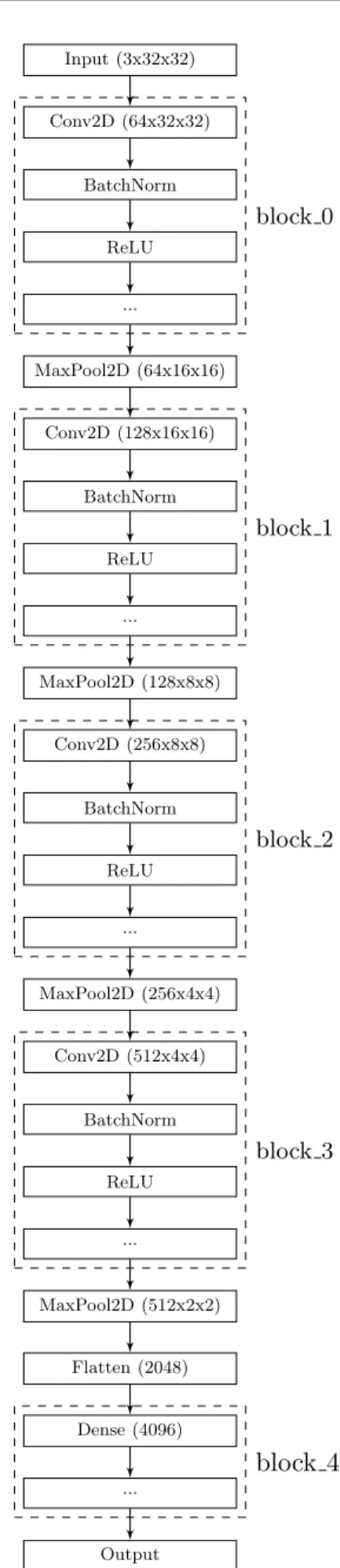
[0,1,2,3]respectively. For the downsampling layers, we use max pooling with kernel size(2×2)and stride(2×2). If we were to scale up the experiments to larger images, we would look to add additional subsampling layers to decrease the spatial size of the feature maps, increase receptive field sizes, and create more tuneable blocks in our architecture. The skeleton architecture which is used as the starting point for the deep CNN evolution can be seen in Fig.3, with further detail in Table.1.
Next, we define a method for mapping a vector of integers to a full convolutional architecture by ‘stacking’ layers in each block, according to the value in the specific index of the architecture vector. In this way, we can explore an
n dimensional space, where n represents the number of tuneable blocks in our architecture. We then frame the task of generating the architecture of a model as a minimisation of an objective function f(x) (defined in Fig.4), where x
represents an abstraction of network architecture into a single point in the navigable multi-dimensional search space and
f(x)represents the error rate of the model when evaluated on the validation set. This involves discovering the optimal value of xwhich produces the minimal error rate when evaluated using the fitness function, as shown by (3).
argmin x
f(x) ={x|x∈S∧∀y∈S:f(y)≥f(x)} (3)
Table. 1: The structure of the convolutional architecture to be optimised when applied to CIFAR-10 and CIFAR-100
layer type input convolutional convolutional convolutional convolutional fully-connected output
depth (no. f-maps) 3 64 128 256 512 4096 10|100
spatial-size (of f-maps) 32×32 16×16 8×8 4×4 2×2 1 1
filter-size n/a 3×3 3×3 3×3 3×3 n/a n/a
block-size (no. layers) n/a 1. . .10 1. . .10 1. . .10 1. . .10 1. . .10 n/a
where,
S⊂Nn | ∀x∈S : 0≤ {x0, . . . , xn−1}<10 (4) in actual fact, we explore the search space using,
S⊂Rn | ∀x∈S : 0≤ {x
0, . . . , xn−1}<10 (5)
and rely on the implicit integer-cast to function as a form of regularisation by only allowing large, or multiple small, movements to modify the structure, similar to the approach taken by [25]. We do this by min-max scaling the position values into our desired range and then converting into inte-gers representing the number of layers to add to each block. This is simply performed by multiplying each position value by the upper bound of the range, as we use the values0and1 as the lower and upper bounds for optimisation respectively. In order to optimise the objective function, we use the pre-viously described evolutionary optimisation technique, i.e. the proposed adaptive PSO model, to efficiently explore the search space defined by our objective function.
B. ENHANCED PARTICLE SWARM OPTIMISATION We propose an enhanced PSO model for optimal deep CNN model generation. It considers each individual architecture in the search space as a position in ann-dimensional space wherenrepresents the number of distinct blocks in our skele-ton architecture. Instead of using fixed acceleration coeffi-cients as in the original PSO model, adaptive search parame-ters based on linear and non-linear functions are proposed. Four new strategies have been applied for the coefficient generation: (1) linear functions with an equal crossover in the centre, (2) cosine functions with an equal crossover in the centre, (3) cosine functions with a later crossover, and (4) cosine functions with no crossover. These strategies are described in further detail in Section III-D.
We start by initialising a population of m individual particles as random positions in the search space, where each dimension in each particle is drawn from a uniform distribution:
X=U(bl, bu) (6)
wherebl andbu are the lower and upper boundaries of the
search space, respectively. We then initialise the velocities of each of the particles:
Vi=U(vmin, vmax) (7)
where,
vmax=λ(bu−bl)
vmin=−vmax
(8)
and we use a value of0.2forλin all experiments based on best practice.
Once the swarm has been initialised, the optimisation process can begin. It starts with updating the inertia weight and both acceleration coefficients according to the specific strategies chosen. Next, each particle Xi is processed with
the following steps. First, the velocity of the particle is updated using the search weights and the distances between the current position and the local and global best positions as defined in (1). Using the velocity, the new position of the particle is calculated based on the previous position as illustrated in (2). The fitness of the particle is evaluated using the objective function provided in Fig.4. The fitness score of
Xi is compared against those of the previous personal best
position Pi and the global best solution, respectively. The
local best position is updated according to (9).
Pi=
(
Xi, iff(Xi)< f(Pi)
Pi, otherwise
(9) Whilst the global best is similarly updated according to (10).
G= argmin Pi f(Pi), if min f(Pi) < f(G) G, otherwise (10)
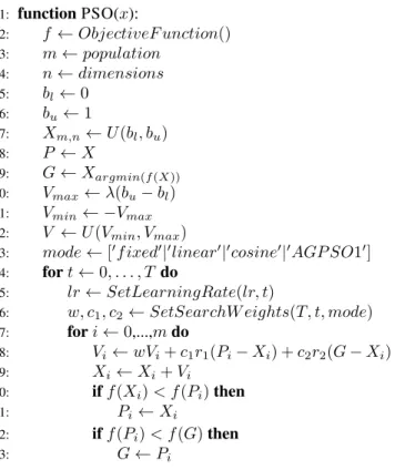
In practice, in order to avoid unnecessary overhead we store the fitness values for each evaluation for the score comparisons, rather than re-calculating the fitness for each updated particle position. This process then repeats over all particles, and all iterations, until a certain stop criterion has been met, i.e. the maximum number of iterations. Once the iterations have completed, the final output of the system is the global best position G and its fitness value f(G), representing the best arguments to minimise the objective function (argminxf(x)) and the fitness value respectively. As mentioned earlier, Section III-D outlines several linear and cosine annealing mechanisms that are proposed for adaptive acceleration coefficient generation in the proposed PSO model to enable the search to balance well between local exploitation and global exploration. Fig.5 demonstrates the proposed, customised PSO, with Fig.4 comprising our bespoke objective function. In comparison with [31], we also employ weight sharing strategies to overcome the function-evaluation cost constraints, which are introduced below.
C. CONTINUAL TRAINING/PARAMETER SHARING Due to the nature of our fitness function, evaluating fully for each particle requires inhibitive amounts of time and resources as each architecture must be trained and validated to obtain a fitness score. We reconcile this constraint through
Input (3x32x32) Conv2D (64x32x32) BatchNorm ReLU ... MaxPool2D (64x16x16) Conv2D (128x16x16) BatchNorm ReLU ... MaxPool2D (128x8x8) Conv2D (256x8x8) BatchNorm ReLU ... MaxPool2D (256x4x4) Conv2D (512x4x4) BatchNorm ReLU ... MaxPool2D (512x2x2) Flatten (2048) Dense (4096) ... Output block 0 block 1 block 2 block 3
block 4
Fig. 3: The skeleton architecture used in the proposed system
the use of early evaluation of the function on the validation set, similar to the approach used by [31]. However, using early evaluation solely does not provide a realistic view of the performance of the particle, as an architecture may train very successfully initially but later plateau before reaching an acceptable level of accuracy. In contrast to [31], we additionally use a form of parameter sharing, allowing new architectures to inherit the weights from previous particles when performing their fitness function evaluations. This al-lows the architectures to train alongside the optimisation process, with each block keeping track of its own weights. In this way, the fitness function evaluations are representative of the performance of the individual particles at all stages of the optimisation process, as their training progresses and perfor-mance increases throughout. In [25], Real et al. implemented weight inheritance as a feature of the inheritance process of their GA, allowing weights for layers with matching shapes to be inherited, or not depending on the specific mutation. We take this a step further by considering weight sharing as a means of continually training all of the models jointly. This continual training allows us to consider the optimisation process as the bulk of the training of the final model, with the fitness function evaluations becoming more accurate as training progresses and the shared weights are trained. This allows us to quickly navigate the search space, following the path that leads to the greatest performance increases as we go. We combine this approach with a previously men-tioned annealing strategy applied to the PSO search weights. These adaptive search parameters in PSO enable the search to favour local exploitation in early iterations and global exploration in final iterations. In this way we ensure that we avoid prematurely optimising to a local minimum before the possible architectures have been trained for a reasonable number of iterations. Without this strategy, it is likely that the large improvements in error rate that can be seen with the first few training iterations would result in a rapid clustering of all of the particles into one area after following the global best solution.
We jointly train the population of continually evolving net-work architectures by maintaining a lookup table of convo-lutional filter parameters and fully-connected layer weights. The lookup table consists of a simple key-value store, where the key takes the form of a string concatenation of the integer block number in the architecture, with the integer size of the block (i.e. the number of layers in the block minus 1; zero indicates a single layer) separated by a period. A key thus takes the form ‘ψ.(ω −1)’ where ψ is the specific number of the block in the skeleton architecture, and ω is the number of layers in the block. Each value in our key-value store is itself a smaller key-key-value store, consisting of two key-value pairs, i.e. the best performing parameters, and the last used parameters, for each distinct block & size. This allows us to check if a specific block has been constructed to a certain size before, and inherit the weights of that block, thereby gradually training the individual blocks as we explore the architecture search space. Initially we experimented with
1: functionOBJECTIVEFUNCTION(position):
2: model←InitM odel(position) .Initialise the model using the particle position vector
3: ifweight_sharingthen
4: model.weights←BlockLookup(position) .Construct the weight lookup keys from the model structure
5: .Determine the weight lookup strategy
6: .Iteratively check the weight lookup table for existing weights
7: .Load the existing weights into the model
8: T rain(model) .Train the model for a single epoch (or a defined number of batches)
9: error_rate←V alidate(model) .Evaluate the model on the validation set to determine the error rate
10: ifweight_sharingthen
11: BlockStore(position, model.weights, error_rate) .Iteratively update the weights in the weight lookup table
12: return(error_rate/100) .Return the error rate as the fitness for this function evaluation Fig. 4: The bespoke objective function to be optimised
1: functionPSO(x): 2: f ←ObjectiveF unction() 3: m←population 4: n←dimensions 5: bl←0 6: bu←1 7: Xm,n←U(bl, bu) 8: P ←X 9: G←Xargmin(f(X)) 10: Vmax←λ(bu−bl) 11: Vmin← −Vmax 12: V ←U(Vmin, Vmax)
13: mode←[0f ixed0|0linear0|0cosine0|0AGP SO10]
14: fort←0, . . . , Tdo
15: lr←SetLearningRate(lr, t)
16: w, c1, c2←SetSearchW eights(T, t, mode)
17: fori←0,...,mdo 18: Vi←wVi+c1r1(Pi−Xi) +c2r2(G−Xi) 19: Xi←Xi+Vi 20: iff(Xi)< f(Pi)then 21: Pi←Xi 22: iff(Pi)< f(G)then 23: G←Pi
Fig. 5: The proposed PSO model with adaptive acceleration coefficients
storing the best performing weights for each particle position & block size (with the error-rate of the model as performance indicator). This approach has the downside of limiting the exploration of the model since it ensures that any training run that does not increase performance by the end of the run will be discarded, in favour of the original parameters. The model is then limited in its exploration capability. To alleviate this issue, we also store the last known weights of each block number & size. We can then choose whether to continue with the last known weights, or to select the best seen so far. We control the selection of existing parameters through a weight valueβ which controls how likely we are to select the best
1: functionLOOKUP(β) 2: ifβ > U(0,1)then 3: returnbest
4: else
5: returnlast
Fig. 6: The weighted parameter lookup function
weights over the last known weights by comparing with a random value between0and1. This process can be seen in Fig.6.
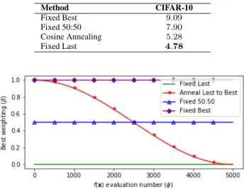
We experimented with a number of strategies forβ. Ini-tially we chose to always use the best weights that have been seen before for each block when performing the inheritance process. However, as previously described, this led to a cycle of limited exploration, whereby a model would become stuck repeatedly retraining parameters but never achieving a better validation score, therefore discarding its progress. Next we experimented with a fixed 50:50 chance of inheritance from best or last, allowing for exploration but also promoting superior results with an even chance. We found this approach to perform better than just using the best results but we still hypothesised that there would be a superior approach. We then implemented an annealing schedule for β, in order to allow the chance of inheriting from best, rather than last, to gradually increase from 0%to100%. This schedule can be seen in (11).
β= 1 + cos(π(1−
φ Φ))
2 (11)
where φ andΦ represent the current and total number of fitness function evaluations respectively.Φcan be calculated bym+m×T, wheremrepresents the swarm population andTrepresents the number of iterations for the optimisation algorithm. Finally, we experimented with only using the last values stored for each block, regardless of their fitness value. Surprisingly, we found this approach to be the most performant, which led to its subsequent use in all following experiments. The four main techniques that were tested can be seen in Fig.7 and the experimental results can be seen in Table.2. When storing the weights for a specific block in
Table. 2: Error Rates (%) for Different Weight Lookup β Strategies Method CIFAR-10 Fixed Best 9.09 Fixed 50:50 7.90 Cosine Annealing 5.28 Fixed Last 4.78
Fig. 7: The different weighting strategies for parameter lookup table access (β for the lookup function) against the number of fitness function evaluations (φ)
the architecture, we transfer the weight tensors into RAM in order to save the on-board GPU memory for larger batch sizes and larger potential network architectures.
Once our optimisation process has concluded, we need to finalise the model for testing. In related work, this is usually performed by discarding any parameters learned during the optimisation process, taking the best architecture discovered, and training it completely from scratch. We use a different approach in order to combine the optimisation process with the final model training, so as not to waste the training progress thus far. We construct a fine-tuning dataset from the previous training and validation sets by combining them into one large training dataset. We then fine-tune the best performing model from the optimisation process on this dataset for a small number of epochs in order to alleviate the effect of any overfitting introduced by the optimisation process. Once we have completed our fine-tuning on the larger training set, we are able to test the model on the test set and report the final results of the model without re-creating or re-training the model after the optimisation process.
D. ADAPTIVE PSO SEARCH WEIGHTS
Using the process outlined above, we are able to effectively explore our constructed search space in reasonable time using the proposed PSO model. In the original PSO model, the search weights for cognitive and social components are fixed when updating the velocity of each particle, which is then used to update the position. Specifically, the coefficients are set to give fixed weightings to both the local and global best solutions for each particle when performing the update. Our continual training method means that initially, we expect to see large gains no matter where a particle moves, owing to the initial training of the networks up to a reasonable level
of performance. Because of this, it is desirable that each particle can be allowed to explore its own space initially, rather than move towards the global best. This will ensure that the particles perform useful exploration in these initial stages, by moving towards the area with the greatest improve-ments around themselves. We can ensure that this happens by setting the ratio between the local search weight and the global search weight to a high value. This could be achieved by setting the local search weight to a fixed, high value and the global search weight to a fixed, low value. However, later in the training process, we expect that the performance gains from each iteration will slow down significantly, as the net-works come closer to achieving their optimal performance. At this point, it is desirable that we obtain the best perform-ing, single network from the population of individuals. It follows then, that rather than allowing the particles to explore around their own space, it would be beneficial to exploit one of the key functions of PSO, by allowing the particles’ positions to trend towards the position of the best performing particle, in the hopes that they can explore together around the position and achieve even better performance. At this later iteration stage, we would like the previously described ratio between local and global search weights to reverse, promot-ing a high ratio of global to local. This means that a fixed ratio for the whole optimisation process is less than ideal, as this reversal process cannot happen. In order to achieve the above, desired outcome for the search weight strategy and overcome the premature convergence of the original PSO model, we explored the concept of adaptive acceleration coefficients, where the search weights can change depending on the current iteration number.
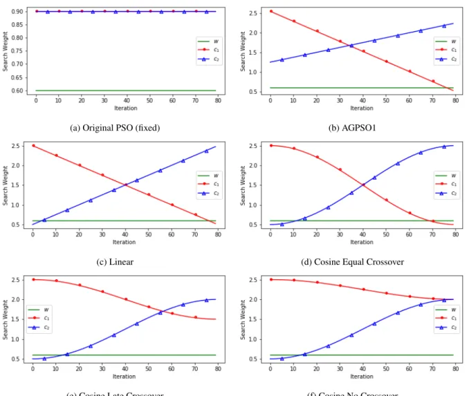
Motivated by [35], several adaptive acceleration coeffi-cient generation schemes are subsequently explored in this research. Fig.8 shows the explored mechanisms for coef-ficient generation, i.e. (1) fixed acceleration coefcoef-ficients in Fig.8a, as the baseline wherec1 =c2 = 0.9andw= 0.6; (2) a linear AGPSO1 schedule borrowed from [35] (in Fig.8b), as another baseline; (3) a proposed linear crossover function in Fig.8c; and (4)-(6) proposed nonlinear cosine annealing schedules with equal, late, and no crossover in Fig.8d, Fig.8e, and Fig.8f respectively. The above adaptive search strategies are employed with the goal of allowing the particles to explore in their local search space initially, so as not to prematurely head towards the global best during the initial training stages. This could happen due to the large increases in accuracy that are present in the initial training steps of a convolutional architecture, combined with our continual training method. We found that maintaining a reasonably high level of local exploration during the optimisation pro-cess was effective to allow the particles to efficiently cover the search space, as can be seen in Fig.9 as well as Fig.10 (with detailed explanation provided later in this section). The proposed linear and nonlinear adaptive search weight functions are provided in (12) and (14), respectively. Fig.11 shows the pseudo-code for the overall adaptive accelera-tion coefficient generaaccelera-tion funcaccelera-tion, with the accompanying
graphs in Fig.8. First of all, the proposed linear coefficient generation function is defined in (12):
c1=Q− t T(Q−q) c2=q+ t T(Q−q) (12)
where t refers to the current iteration number, T refers to the total number of iterations to be performed for the optimisation run,qrefers to the lower bound for the search weight, andQrefers to the upper bound for the search weight. A baseline adaptive weight generation strategy of AGPSO1 from [35] is defined below:
c1=t 1 T + 1.25 c2=t −2.05 T + 2.55 (13)
Motivated by (13), in order to adapt the weights more gently towards the extreme values, a smoother annealing schedule is proposed in this research, based on the cosine function. (14) denotes the proposed cosine search weights and variants:
c1=q+ Q−q 2 cos(π(1− t T)) + 1 c2=q+ Q−q 2 cos(π t T) + 1 (14)
where the variants are created by choosing different values forqandQforc1andc2. The Cosine Equal Crossover variant
(Fig.8d) is created usingq= 0.5,Q= 2.5for bothc1andc2.
The Cosine Late Crossover variant (Fig.8e) is created using
q = 1.5,Q = 2.5 for c1 andq = 0.5,Q = 2.5 for c2.
The Cosine No Crossover variant (Fig.8f) is created using
q = 2.0,Q = 2.5 for c1 andq = 0.5,Q = 2.5 for c2.
As mentioned above, Fig.11 shows the pseudo-code of the adaptive weight generation over iterations, which are then used to update the velocities of the particles using (1).
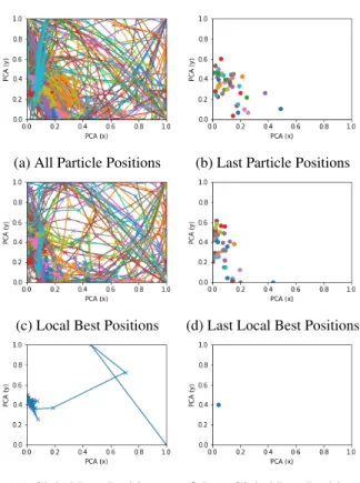
With fixed search weights, the behaviour of particles with respect to local or global exploration remains the same throughout the optimisation process, favouring whichever is given a higher weighting, or neither if they are equally weighted. Using an annealing schedule allows us to intro-duce different search behaviour trends on local and global exploration that evolve over the course of the optimisation. Specifically we utilise this for the linear, AGPSO1, and cosine schedules to initially favour local exploration around each particle’s own best position, and gradually trend towards focusing on global exploration, towards the best particle position found so far. We do this to prevent our particles from quickly abandoning their local search space in favour of pursuing the best position, and thereby all becoming stuck in the same local minima. Fig.10 demonstrates the effects of the late crossover cosine search weight strategy on the local bests of each particle and the overall global best. The
xandy axes represent the particle positions projected into two-dimensional space using Principal Component Analysis (PCA). Thezaxis represents the fitness value for the particle
Table. 3: Error rates (%) for different search weight strategies
Method CIFAR-10
Original PSO (fixed) 5.38
AGPSO1 [35] 5.84
Linear Crossover 5.78 Cosine Equal Crossover 5.14 Cosine Late Crossover 4.78
Cosine No Crossover 10
after being evaluated on the validation set. Fig.10a shows how initially the particles explore their own space, improving their fitness scores but not converging on a single location, as well as how they begin to converge on the xandy axes later as the search weights begin to favour following the global best. This can also be seen in the positions of the local and global bests in Fig.10b and Fig.10c, which eventually converge around a single point after gradually narrowing focus and improving fitness scores.
The test results for the different strategies for adaptive coefficient generation can be seen in Table.3.
E. HYPERPARAMETERS
We use the excellent PyTorch library [36] for all deep learning implementation and training. Each particle fitness function evaluation involves creating a full CNN architec-ture from the particle representation, training the CNN us-ing stochastic gradient descent with backpropagation, and evaluating the CNN on the validation set to determine its fitness score. Treating the CNN training as a ‘black box’ like this means that our method could be generalised to other deep learning tasks, where the fitness function could be modified to train a different type of network without having to modify the PSO system. We train each individual CNN model using stochastic gradient descent (SGD) with a nesterov momentum factor [37], [38] of 0.9, and weight decay (L2 regularisation) of 1e-4, on minibatches of size 256 for one epoch per fitness function evaluation. The proposed PSO swarm optimisation is performed using a population size of 50 individual particles with a maximum number of iterations of 100.
1) Learning Rate
In this research, we also experimented with a number of different approaches for the learning rate schedule in order to find the best mechanism for our combined optimisation and training process. We started with (1) simple scheduled learn-ing rate decay at certain points in the optimisation/trainlearn-ing process using (15), αφ = ( γαφ−1, ifφ= 50orφ= 75 αφ−1, otherwise (15) whereγwas set to10−1and the initial learning rate was also
set to10−1. This approach was reasonably effective.
Motivated by [39], [40], we experimented with (2) cyclic learning rates, which proved effective owing to the fast ini-tial convergence, allowing the shared parameters to quickly
(a) Original PSO (fixed) (b) AGPSO1
(c) Linear (d) Cosine Equal Crossover
(e) Cosine Late Crossover (f) Cosine No Crossover
Fig. 8: PSO search weights by iteration
become effective. Huang et al. [39] use a cyclical learning rate to repeatedly train a network to an acceptable level of performance, then store a snapshot of the model in that state. These snapshots are then combined into an ensemble model in a manner similar to gradient boosting, to achieve enhanced performance. They construct an ensemble by ‘snapshotting’ the parameter weights after each cycle of the learning rate, although we found it effective to simply train our models with shared parameters using the cyclic learning rate without snapshotting. The cyclic learning rate that we used in our experiments can be seen in (16).
αφ=
α0
2 (cos(
πmod(φ−1,dΦ/Me)
dΦ/Me ) + 1) (16)
whereM represents the number of cycles, which was set to 5in our experiments.
Our final approach for the learning rate was to simply use (3) cosine annealing to decrease the learning rate over a defined interval, throughout the optimisation process. This
was performed using (17),
αφ =b+
a−b
2 cos(π
φ
Φ) + 1 (17)
where a and b represent the initial and final learning rate values respectively, for the interval. We found this approach works best for our combined optimisation and training pro-cess, with values of10−1and10−4foraandbrespectively.
Therefore, all of the following reported results use this strat-egy. We also used this decay strategy for the fine-tuning portion of the model training, using values of10−4and10−7
foraandbrespectively. A visualisation of the three different learning rate schedules can be seen in Fig.12.
2) Fine-tuning
As previously mentioned, the usual method for evaluating ar-chitecture optimisation systems is to separate out the optimi-sation process from the final model training process. Contrary to this approach, we evaluate our optimisation process by integrating it into the training process for the final model to be
(a) All Particle Positions (b) Last Particle Positions
(c) Local Best Positions (d) Last Local Best Positions
(e) Global Best Positions (f) Last Global Best Positions
Fig. 9: Example particle movements over time (PCA for dimensionality reduction to display particle positions on two axes)
tested. Once the optimisation process has completed, we then fine-tune the best performing model on a combined training set consisting of the training and validation sets together for a small number of epochs. In this way the training of the final network is embedded in the optimisation process, meaning the architecture design and training are performed as one task. By using this approach we couple the architecture de-sign and training processes together and remove some of the high barrier-to-entry for building CNNs for new problems. The finetuning process is performed for 10 epochs and uses SGD with a nesterov momentum factor of 0.9, and weight decay (L2 regularisation) of 1e-4, on minibatches of size 256 with a cosine annealing learning rate schedule over an interval ofa= 10−4andb= 10−7.
IV. EVALUATION
The well known CIFAR-10 and CIFAR-100 datasets [7] are used to evaluate the proposed SOBA model.
The CIFAR-10 dataset consists of 60,000 images equally split over 10 classes (6,000 per class). The dataset divides into 50,000 training images and 10,000 test images. For our experiments we further divided the 50,000 training im-ages into 45,000 training and 5,000 validation, whereby the validation set was used to generate the fitness scores for each function evaluation in the optimisation process. Fig.13a shows a confusion plot generated from thepre-fine-tuning
(a) Local best positions & their fitness scores by iteration for all 50 particles (point indicates start position)
(b) All local & global best positions & their fitness scores
(c) Global best positions & their fitness scores
Fig. 10: Example local and global best positions over time (PCA for dimensionality reduction to display particle posi-tions on two axes)
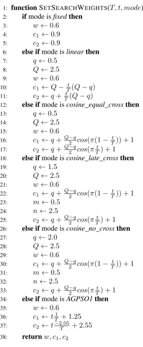
1: functionSETSEARCHWEIGHTS(T, t, mode) 2: ifmode isfixedthen
3: w←0.6
4: c1←0.9
5: c2←0.9
6: else ifmode islinearthen
7: q←0.5 8: Q←2.5 9: w←0.6 10: c1←Q− t T(Q−q) 11: c2←q+ t T(Q−q)
12: else ifmode iscosine_equal_crossthen
13: q←0.5
14: Q←2.5
15: w←0.6
16: c1←q+Q−q2 cos(π(1−Tt)) + 1
17: c2←q+Q−q2 cos(πTt) + 1
18: else ifmode iscosine_late_crossthen
19: q←1.5 20: Q←2.5 21: w←0.6 22: c1←q+Q−q2 cos(π(1− t T)) + 1 23: m←0.5 24: n←2.5 25: c2←q+Q−q2 cos(πTt) + 1 26: else ifmode iscosine_no_crossthen
27: q←2.0 28: Q←2.5 29: w←0.6 30: c1←q+Q−q2 cos(π(1−Tt)) + 1 31: m←0.5 32: n←2.5 33: c2←q+Q−q2 cos(πTt) + 1
34: else ifmode isAGPSO1then
35: w←0.6
36: c1←tT1 + 1.25 37: c2←t−2.05T + 2.55 38: returnw, c1, c2
Fig. 11: The function for the generation of adaptive PSO search weights
Fig. 12: Learning rate by iteration
test on the CIFAR-10 dataset, whilst (18) shows the raw confusion matrix. 933 0 119 24 4 819 6 20 12 2 18 15 2 4 0 1 0 0 965 947 0 1 0 0 0 0 0 0 0 4 1 963 30 94 22 122 990 4 8 17 0 0 0 0 0 0 0 0 0 0 12 21 834 15 14 6 1 20 9 12 0 0 0 0 0 0 0 0 0 0 0 0 0 0 0 0 0 0 0 0 32 0 5 846 7 39 1 19 6 16 4 0 10 17 953 13 2 937 0 2 (18) This test was not used to influence the fine-tuning in any way. It was simply performed in order to demonstrate the effect of fine-tuning on the classification performance. Fig.13b shows the confusion plot generated after fine-tuning, with (19) showing the accompanying raw confusion matrix.
965 1 7 6 3 2 3 4 16 4 1 979 0 1 0 0 0 0 5 22 13 0 934 18 8 9 8 4 5 1 2 0 14 878 9 41 8 8 2 1 1 1 15 16 966 12 3 12 0 0 0 0 13 64 8 930 1 9 0 1 1 0 10 7 2 3 975 1 0 0 0 0 3 5 3 2 2 961 0 0 16 3 3 4 1 1 0 0 968 5 1 16 1 1 0 0 0 1 4 966 (19) Table.4 shows aggregate statistics for the CIFAR-10 test runs before the fine-tuning process and after. It is clear that the fine-tuning process is effective in reversing the overfitting on the training set and allows the model to generalise to greatly improved performance on the test set. This fast, effective gen-eralisation is owing to the robustness of the weights learned through our combined optimisation and training process, as each block in the architecture is trained to be globally optimal for all potential surrounding configurations, rather than one single, fragile configuration. It is also interesting to note that after fine-tuning, the areas that the model seems to struggle, namely the intersections of cat-dog, ship-airplane, and truck-automobile, are areas that intuitively would also prove difficult to a human classifying the images by hand.
The CIFAR-100 dataset consists of the same number of images but split over 100 classes, each of which belongs to one of twenty ‘superclasses’. Each class has 500 train-ing images and 100 testtrain-ing images, resulttrain-ing in the same training-testing split as that of CIFAR-10 (50,000 vs 10,000 respectively). As with CIFAR-10, we further split the training images into 45,000 training and 5,000 validation for CIFAR-100, and the validation images are used to generate the model fitness after each optimisation function evaluation.
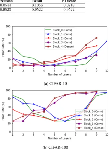
Fig.14 shows some analysis of the lookup table following the final access during the optimisation/training process. Each line represents a different block in the architecture,
Table. 4: Aggregate performance measures on the CIFAR-10 test set
Stage Accuracy Error Rate Macro-Average Precision Macro-Average Recall Macro-Average F1 Score Pre-fine-tuning 10.56% 89.44% 0.0544 0.1056 0.0718 Post-fine-tuning 95.22% 4.78% 0.9523 0.9522 0.9522 (a) Pre-Finetuning (b) Post-Finetuning
Fig. 13: Confusion plots for CIFAR-10 test results
(a) CIFAR-10
(b) CIFAR-100
Fig. 14: The best validation error rates achieved for each individual block during the optimisation process, from the final lookup table
with the number of layers in the block displayed along the x axis. The y axis shows the lowest error rate achieved by any particle with that configuration of block in its architecture (although the other blocks could be in any configuration). It is clear from the CIFAR-10 experiment (Fig.14a) that the system tends to prefer more depth in the initial blocks, whilst the feature maps are larger and the receptive field is smaller, and more shallow blocks later in the network, especially when it comes to the fully connected layers. This becomes drastically more pronounced in the CIFAR-100 experiment (Fig.14b) when the number of output classes is increased by an order of magnitude and the same pattern can still be seen.
We have also compared our model with related research as illustrated in Table.5. The first section of the table con-tains traditional, hand-crafted architectures, the second sec-tion contains reinforcement learning (RL) techniques, the third section contains evolutionary techniques, and the final section contains our proposed model. In comparison with most of the existing studies, our proposed model achieves the best trade-off between performance and computational efficiency. As an example, [26], [25], and [19] used 200,
Table. 5: Classification error rates (%) for the proposed SOBA model and other related studies
Method CIFAR-10 CIFAR-100 GPUs Time (hours)
Handcrafted architectures
VGG [6] 7.25 - n/a n/a
ResNet-110 [9] 6.61 - n/a n/a
WideResNet [41] 3.80 18.30 n/a n/a
DenseNet [42] 3.46 17.18 n/a n/a
Reinforcement learning techniques
MetaQNN [18] 6.92 27.14 10 10
Neural Architecture Search [19] 3.65 - 800 672
Evolutionary optimisation techniques
Large-Scale Evolution [25] 5.40 23.00 250 264 Block-QNN [21] 3.54 18.06 32 72 SMASHv1 [27] 5.53 22.07 - -SMASHv2 [27] 4.03 20.60 - -Genetic CNN [43] 7.10 29.03 ∼20 ∼24 Hierarchical Representations [26] 3.60 - 200 36 Our system
SOBA (inc training model) 4.78 25.42 1 34
(36for C-100)
250, and 800 GPUs with 36, 264, and 672 processing hours respectively, but in some cases the performance enhancement was marginal. Whilst these works did allow for more varia-tion in the proposed architectures, they are also inaccessible to the average user due to the enormous cost. They also require re-training from scratch for the eventually discov-ered architectures, whilst our method provides optimisation and training in one process, quickly delivering an effective, trained network. In addition, we also compare against hand-designed methods [6], [9], [41], and [42], where our method creates architectures that are most similar to [6]. However, we achieve much improved results using our combined opti-misation and training strategy and the enhanced PSO model to generate and train the models. This improvement comes not only from the optimised network topology itself, but also from the robustness of the parameters in our network, as each block is trained to its optimal performance regardless of the configuration of the blocks surrounding it, ensuring that we do not train to fragile local minima. Networks such as VGG-16 [6] are likely to train to local minima as the structure of the network never changes during the training process. The integration of an overall optimisation process in SOBA ensures that even as the structure of the network changes, we still strive for the global minimum, thereby avoiding the local minima as they disappear and reappear. This robustness of weights is ideal for transfer learning as the network is already able to deal very effectively with changes in surrounding structure, so adding or removing layers will not disrupt the performance greatly.
V. CONCLUSION
In this research we have presented an enhanced PSO model with adaptive search weights and weight sharing for optimis-ing the architecture of deep image classification networks. Our model starts with a hand-crafted skeleton architecture and quickly explores our constructed search space by con-currently training multiple architectures, using a weighted lookup table of trained parameters. This allows us to optimise
the architecture of CNNs quickly and effectively, without having to fully train and validate each architecture from scratch, which is prohibitively expensive. We demonstrate results on CIFAR-10 and CIFAR-100, with comparison to other recent architecture optimisation studies. As illustrated in Table.5, our proposed model is among the top performers and has significantly lower computational and hardware requirements than those of other methods, even with our method of training and optimising all-in-one, with no sep-aration between the optimisation and training of the final test architecture.
For future work, we intend to explore adding residual con-nections [9] to the architecture search space, in order to investigate the differences on the performance of the search methods. We intend to expand our formulation of the search space to treat the network structure as a Directed Acyclic Graph, rather than a simple hierarchical structure. We also intend to compare the performance of our enhanced PSO method with other, similar optimisation techniques inside our SOBA model on a wider variety of datasets, including trans-fer learning tasks such as facial emotion recognition, image description generation, and visual question generation.
REFERENCES
[1] Y. LeCun, B. Boser, J. S. Denker, D. Henderson, R. E. Howard, W. Hub-bard, and L. D. Jackel, “Backpropagation applied to handwritten zip code recognition,” Neural computation, vol. 1, no. 4, pp. 541–551, 1989. [2] O. Russakovsky, J. Deng, H. Su, J. Krause, S. Satheesh, S. Ma, Z. Huang,
A. Karpathy, A. Khosla, M. Bernstein, A. C. Berg, and L. Fei-Fei, “Im-ageNet Large Scale Visual Recognition Challenge,” International Journal of Computer Vision (IJCV), vol. 115, no. 3, pp. 211–252, 2015. [3] G. A. Miller, “Wordnet: a lexical database for english,” Communications
of the ACM, vol. 38, no. 11, pp. 39–41, 1995.
[4] D. G. Lowe, “Distinctive image features from scale-invariant keypoints,” International journal of computer vision, vol. 60, no. 2, pp. 91–110, 2004. [5] N. Dalal and B. Triggs, “Histograms of oriented gradients for human detection,” in Computer Vision and Pattern Recognition, 2005. CVPR 2005. IEEE Computer Society Conference on, vol. 1. IEEE, 2005, pp. 886–893.
[6] K. Simonyan and A. Zisserman, “Very deep convolutional networks for large-scale image recognition,” CoRR, vol. abs/1409.1556, 2014.