Top-k Exploration of Query Candidates for Efficient Keyword Search on Graph-Shaped (RDF) Data

Top-k Exploration of Query Candidates for Efficient

Keyword Search on Graph-Shaped (RDF) Data

∗

Thanh Tran

_{, Haofen Wang}

_{, Sebastian Rudolph}

_{, Philipp Cimiano}

Universit¨at Karlsruhe, Germany

{dtr,sru}@aifb.uni-karlsruhe.de 2_{Department of Computer Science & Engineering}

Shanghai Jiao Tong University, Shanghai, 200240, China [email protected]

3_{Web Information Systems}

TU Delft, PO Box 5031, 2600 GA Delft, The Netherlands [email protected]

Abstract— Keyword queries enjoy widespread usage as they represent an intuitive way of specifying information needs. Recently, answering keyword queries on graph-structured data has emerged as an important research topic. The prevalent approaches build on dedicated indexing techniques as well as search algorithms aiming at finding substructures that connect the data elements matching the keywords. In this paper, we introduce a novel keyword search paradigm for graph-structured data, focusing in particular on the RDF data model. Instead of computing answers directly as in previous approaches, we first compute queries from the keywords, allowing the user to choose the appropriate query, and finally, process the query using the underlying database engine. Thereby, the full range of database optimization techniques can be leveraged for query processing. For the computation of queries, we propose a novel algorithm for the exploration of top-kmatching subgraphs. While related techniques search the best answer trees, our algorithm is guaranteed to compute all k subgraphs with lowest costs, including cyclic graphs. By performing exploration only on a summary data structure derived from the data graph, we achieve promising performance improvements compared to other approaches.

I. INTRODUCTION

Query processing over graph-structured data has attracted much attention recently, which can be explained by the mas-sive availability of such type of data. For instance, XML data can be represented as graphs. In many approaches, even databases have been treated as graphs, where tuples correspond to vertices and foreign relationships to edges (see [1], [2]).

A data model that explicitly builds on graphs is RDF1_{, a} framework for (Web) resource description standardized by the W3C. RDF appears to have a great momentum on the web and an increasing amount of data is becoming available. The RDF model has also attracted attention in the database community. ∗_{This work has been supported by the European Commission under contract}

IST-FP6-026978 X-Media, and by the Deutsche Forschungsgemeinschaft (DFG) under the ReaSem project.

1_{http://www.w3.org/RDF/}

Recently, many database researchers have proposed solutions for the efficient storage and querying of RDF data (e.g. [3], [4], [5]).

In this paper, we present an approach for keyword search on graph-structured data, RDF in particular. Query mechanisms that are accessible to ordinary users have always been an important goal of database research. Relaxed-structure query models aim at facilitating the construction of complex queries (SQL or XQuery) by supporting relaxed patterns as well as structure-free query components. Labelled query models do not require any knowledge about the structure as the user simply associates values with schema elements called “labels”. At the end of the spectrum, keyword search does not require any knowledge about the query syntax or the schema.

Much work has been carried out on keyword search over tree-structured data (e.g. [6], [7], [8], [9], [10], [11], [12], [13]) as well as graph-structured data (e.g. [2], [14], [1]). The basic idea is to map keywords to data elements (keyword elements), search for substructures on the data graph that connect the keyword elements, and output the top-k substructures com-puted on the basis of a scoring function. This task can be decomposed to 1) keyword mapping, 2) graph exploration, 3) scoring and 4) top-kcomputation.

In many approaches ([1], [14]), anexact matching between keywords and labels of data elements is performed to obtain the keyword elements. For the exploration of the data graph, the so-called distinct root assumption is employed (see [2], [1], [14]). Under this assumption, only substructures in the form of trees with distinct roots are computed and the root element is assumed to be the answer. The algorithms for finding these answer trees are backward search ([1]) and bidirectional search ([14]). For top-kprocessing and ranking, different scoring functions have been proposed (see [6], [9], [8], [11], [15], [10], [12], [16]), where metrics range from path lengths to more complex measures adopted from IR. In order to guarantee that the computed answers indeed have the best

scores, both the lower bound of the computed substructures and the upper bound of the remaining candidates have to be maintained. Since book-keeping this information is difficult and expensive, current algorithms compute the best answers only in anapproximate way (see [1], [14]).

In our approach, IR concepts are adopted to support an imprecise matching that incorporates syntactic and semantic similarities. As a result, the user does not need to know the labels of the data elements when doing keyword search. We now present our main contributions to keyword search on graph-structured data:

• Keyword Search through Query Computation While

the mentioned approaches interpret keywords as neigh-bors of answers, we interpret keywords as elements of structured queries. Instead of presenting the top-k

answers, which might actually belong to many distinct queries, we let the user select one of the top-kqueries to retrieve all its answers. Thus, the keyword search process contains an additional step, namely the presentation of structured queries. We consider this step as beneficial because queries can be seen as descriptions, and can thus facilitate the comprehension of the answers. Also, refinement can be made more precisely on the structured query than on the keyword query.

• Algorithms for Subgraph ExplorationOur main

techni-cal contribution is a novel algorithm for the computation of the top-ksubgraphs. In current approaches, keywords are exclusively mapped to vertices. In order to connect the vertices corresponding to the keywords, current algo-rithms aim at computing tree-shaped candidate networks ([10], [6], [9]) or answer trees ([1], [14], [2]). Since keywords do not necessarily correspond to answers ex-clusively in our approach, they might also be mapped to edges. As a consequence, substructures connecting keyword elements are not restricted to trees, but can be graphs in general. Thus, algorithms as applied for tree-exploration such as breadth-first search (e.g. [6], [9]), backward search [1] or bidirectional search [14] are not sufficient.

• Efficient and Complete Top-kthrough Graph

Summa-rizationSo far, algorithms for top-kretrieval assume that the computed substructures connecting keyword elements represent trees with distinct roots (e.g. [1], [2], [14]). Since book-keeping the information required for

top-k processing is difficult and expensive, existing top-k

algorithms (see [14], [1]) can not provide the guarantee that the results indeed have the best scores. This problem is exacerbated when searching for subgraphs. In order to guarantee that the results are indeed top-k subgraphs, we introduce more complex data structures to keep track of the scores of all explored paths and of all remaining candidates. For efficiency reasons, a strategy for graph summarization is employed that can substantially reduce the search space. This means that the exploration of subgraphs does not operate on the entire data graph but a summary containing only the elements that are necessary

to compute the queries.

We have achieved encouraging performance in comparison with previous approaches ([14], [2]). The effectiveness studies show that the generated queries match the meaning intended by the user very well. The user feedbacks on the demo sys-tem available at http://km.aifb.uni-karlsruhe.de/SearchWebDB/ suggest that the presentation of structured queries is valuable in terms of comprehension and enables more precise refine-ment than using keywords.

The rest of the paper is organized as follows. Section II introduces the problem tackled by our approach. Section III provides an overview of the off-line and online computation required in our approach. Details on the computation of the indices, the scores and the matching subgraphs are then provided in Section IV, Section V and Section VI, respectively. Section VII presents evaluation results. Finally, we survey the related work in Section VIII and conclude in Section IX.

II. PROBLEMDEFINITION

We assume that users formulate their information needs using some user query languageQU. Query engines support

queries specified in asystem query languageQS. When these

two languages are different, a transformation is necessary so that the user query can be processed by the system’s query engine. We deal with such scenarios where queries formulated by the user are simply sets of keywords and the query engine supports conjunctive queries only. We elaborate on this keyword search problem in what follows:

DataFor both the translation ofQU toQS and the actual

processing ofQS, we make use of the data graphG, a RDF

data model containing triples.

Definition 1: Adata graphGis a tuple (V, L, E)where

• V is a finite set of vertices. Thereby, V is conceived

as the disjoint unionVE]VC]VV with E-vertices VE

(representing entities), C-vertices VC (classes), and

V-verticesVV (data values).

• Lis a finite set ofedge labels, subdivided byL=LR]

LA] {type, subclass}, whereLR represents inter-entity

edges andLA stands for entity-attribute assignments.

• E is a finite set of edges of the form e(v1, v2) with

v1, v2 ∈V and e∈ L. Moreover, the following

restric-tions apply:

– e∈LR if and only ifv1, v2∈VE,

– e∈LA if and only ifv1∈VE andv2∈VV,

– e=type if and only ifv1∈VE andv2∈VC, and

– e=subclass if and only ifv1, v2∈VC.

The two predefined types of edges, i.e.type andsubclass, have a special interpretation. The former captures the class membership of an entity and the latter is used to define the class hierarchy. Vertices corresponding to entities are identified by specific IDs, which in the case of RDF data are so called Uniform Resource Identifiers (URIs). As identifiers for other elements we use class names, property names, attribute names and values, respectively.

As mentioned, RDF is relevant in practice because of its widespread adoption. Figure 1a shows an example RDF graph,

Sub. Prop. Obj.

pro2URI type Project pro1URI type Project pro1URI name X-Media pub1URI type Publication pub1URI author re1URI pub1URI author re2URI pub1URI year 2006 pub2URI type Publication re1URI type Researcher re1URI name Thanh Tran re1URI worksAt inst1URI re2URI type Researcher re2URI name P. Cimiano re2URI worksAt inst1URI inst1URI type Insitute inst1URI name AIFB inst2URI type Institute Institute subclass Agent Researcher subclass Person Person subclass Agent Agent subclass Thing

Example Keyword Query

2006 c i m i a n o a i f b

Example C o n j u n c t i v e Query

(x, y, z). t y p e ( x , P u b l i c a t i o n ) ∧ y e a r ( x , 2 0 0 6 )

∧ a u t h o r ( x , y ) ∧ name ( y , P . Cimiano )

∧ worksAt ( y , z ) ∧ name ( z , AIFB )

Example SPARQL Query

SELECT ? x , ? y , ? z WHERE{

? x t y p e P u b l i c a t i o n . ? x y e a r 2 0 0 6 . ? x a u t h o r ? y . ? y name ’ P . Cimiano ’ . ? y worksAt ? z . ? z name ’ AIFB ’}

Example SQL Query SELECT A . s . , D . s . , F . s . FROM Ex AS A, Ex AS B , Ex AS C , Ex AS D, Ex AS E , Ex AS F WHERE A . p . = t y p e AND A . o . = P u b l i c a t i o n AND A . s . = B . s . AND B . p . = y e a r AND B . o . = ’2006 ’ AND B . s . = C . s . AND C . p . = a u t h o r AND C . o . = D . s . AND D . p . = name AND D . s . = E . s . AND D . o . = ’ P . Cimiano ’ AND E . p . = worksAt AND E . o . = F . s . AND F . p . = name AND F . o = ’ AIFB ’

Fig. 1. a) Example RDF Data Graph b) Single Table Schema c) Example Queries

containing data about publications, researchers, the institutes they work for etc. Technically, RDF data is often stored in a relational database. For instance, exactly one relational table of three columns can be used to store entities’ properties and attributes (such as in Jena [3], Sesame [17] or Oracle [4]). In our example, the RDF graph is translated to data of the table shown in Fig. 1b. Recently, more advanced techniques such as the property table (c.f. [3], [4]) and vertical partitioning that leverage column-oriented databases have greatly increased performance of storage and retrieval of RDF data [5]. For instance, the required number of self-joins, as apparent in the SQL query shown in Fig. 1c, can be reduced substantially using these techniques.

Queries In our scenario, the user query QU is a set of

keywords(k1, ..., ki). The system queriesQS areconjunctive

queries defined as follows:

Definition 2: A conjunctive query is an expression of the form (x1, . . . , xk).∃xk+1, . . . xm.A1 ∧ . . . ∧Ar, where

x1, . . . , xk are calleddistinguished variables(those which will

be bound to yield an answer), xk+1, . . . , xm are

undistin-guished variables(existentially quantified) andA1, . . . , Arare

query atoms. These atoms are of the form P(v1, v2), where

P is calledpredicate,v1,v2 are variables orconstants.

While variables and constants correspond to identifiers of vertices, predicates correspond to labels of edges in the considered data graph. Conjunctive queries have high practical relevance because they cover a large part of queries issued on relational databases and RDF stores. That is, many SQL and SPARQL queries can be written as conjunctive queries (cf. example query shown in Fig. 1c). SPARQL2 _{is a query} language for RDF data recommended by the W3C.

Answers Since variables can interact in an arbitrary way, a conjunctive query q as defined above can be seen as a graph pattern. Such a pattern is constructed from a set of triple patternsP(v1, v2)in which zero or more variables might

appear. A solution toqon a graphGis a mappingµfrom the 2_{http://www.w3.org/TR/rdf-sparql-query/}

variables in the query to verticese such that the substitution of variables in the graph pattern would yield a subgraph of

G. Thesubstitutions of distinguished variables constitute the answers, which are defined formally as follows:

Definition 3: Given a data graph G = (V, L, E) and a conjunctive queryq, letV ard (resp.V aru) denote the set of

distinguished (resp. undistinguished) variables occurring inq. Then a mappingµ:V ard→V from the query’s distinguished

variables to the vertices of G will be called ananswer to q, if there is a mappingν :V aru→V fromq’s undistinguished

variables to the vertices ofGsuch that the function

µ0:V ard∪V aru∪V →V    v7→µ(v) ifv∈V ard v7→ν(v) ifv∈V aru v7→v ifv∈V satisfies P(µ0_(v 1), µ0(v2))∈E for any P(v1, v2)inq.

Typically, search on RDF data starts with a SPARQL query such as shown in Fig. 1c, which is evaluated by the SPARQL query engine. Using standard rewriting techniques (see [3], [17], [4]), the engine translates the query to SQL and returns the answers as computed by the underlying database engine.

Problem We are concerned with the computation of con-junctive queries from keywords using graph-structured data. We want to find the top-ranked queries, where the ranking is produced by the application of a cost functionC :q→c. For any given query q, Cassigns a cost that captures the degree to which a query qmatches the user’s information need.

III. OVERVIEW OF THEAPPROACH

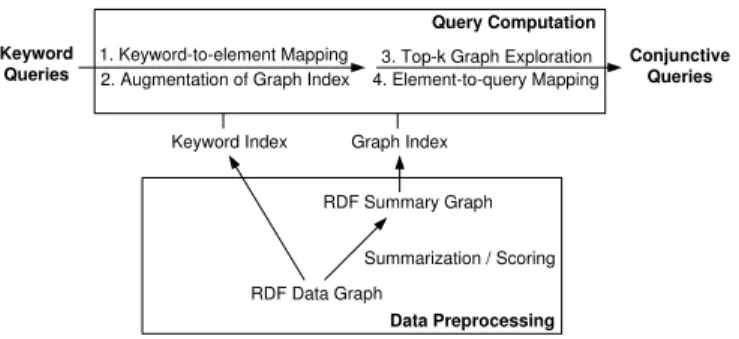
We start with an overview of the different steps involved in our process of keyword search, which is depicted in Figure 2. We will partially illustrate the whole process on the basis of a running example for the query ‘X-Media Philipp Cimiano publications’.

The crucial challenge we address is to infer a structured query from an information need expressed in the form of keywords. For example, the above keyword query asks for

RDF Data Graph

Summarization / Scoring RDF Summary Graph 1. Keyword-to-element Mapping

2. Augmentation of Graph Index

Keyword Index Graph Index

3. Top-k Graph Exploration 4. Element-to-query Mapping Conjunctive Queries Keyword Queries Query Computation Data Preprocessing

Fig. 2. Data Preprocessing and Query Computation

‘publications’that are in the hasProjectrelation with

‘X-Media’ and having author ‘Philipp Cimiano’. However,

there is no reference to the relations hasProject nor to

author in the query. These connections need thus to be inferred to interpret the query correctly. In our previous work [18], [19], we rely on the graph schema to infer such missing connections. In this paper, we are concerned with the challenge of doing this efficiently and propose an approach in which the best interpretations of the query are computed using a top-k

algorithm. We detail the different steps of the approach below.

Query Computation In order to compute queries, the keywords are first mapped to elements of the data graph. From these keyword elements, the graph is then explored to find a connecting element, i.e. a particular type of graph element that is connected to all keyword elements. The paths between the connecting element and a keyword element are combined to construct a matching subgraph. For each sub-graph, a conjunctive query is derived through the mapping of graph elements to query elements. In particular, based on the structural correspondence of triple patterns of a query and edges of the data graph, vertices are mapped to variables or constants, and edges are mapped to predicates. The process continues until the top-k queries have been computed.

PreprocessingIn order to perform these steps in an efficient way, we preprocess the data graph to obtain a keyword index that is used for the keyword-to-element mapping. For exploration, a graph index is constructed, which is basi-cally a summary of the original graph containing structural (schema) elements only. At the time of query processing, this index is augmented with keyword elements obtained from the keyword-to-element mapping. The augmented index contains sufficient information to derive the structure as well as the predicates and constants of the query. Since we are interested in the top-kqueries, graph elements are also augmented with scores. While scores associated with structure elements can be computed off-line, scores of keyword elements are specific to the query and thus can only be processed at query computation time.

Running Example In Fig. 3a, the augmented summary graph is shown for the example RDF data graph in Fig. 1a. This summary graph contains both the structural information computed during preprocessing (rendered gray) and the query specific elements added at query computation time (shown in white). In particular, the keywords of the query given in Fig. 1c

are mapped to corresponding elements of the augmented sum-mary graph, i.e. the vertices v2008, vAIFB andvp.c.. For each

of these keyword elements, the score as computed off-line is combined with the matching score obtained from the keyword-to-element mapping. The graph exploration starts from these three vertices (corresponding to keywords in the query), result-ing in three different paths as shown by the different arrow types in Fig. 3b (note that the arrows indicate the direction of the exploration, not the direction of the edges). Among them, there are three paths that meet at the connecting element nc,

namely p1(AIF B, ..., nc),p2(P hilipp Cimiano, ..., nc)and

p2(2006, year, nc) (rendered bold in Fig. 3b). These three

paths are merged, and the resulting matching subgraph is mapped to the conjunctive query presented in Fig. 1c and illustrated in Fig. 3c. Note that in this case, the matching subgraph is actually a tree. However, keywords elements might be edges that form a cyclic graph. The matching substructure is also very likely to be a graph when keywords are mapped to edges that are loops. We will see that the augmented summary graph might contain many loops.

IV. INDEXINGGRAPHDATA

This section describes the off-line indexing process where graph data is preprocessed and stored in specific data structures of a keyword and a graph index.

A. The Keyword Index

In our approach, keywords entered by the user might refer to data elements (constants) or structure elements of a query (predicates). From the data graph point of view, keywords might refer to C-vertices (classes), E-vertices (entities) or V-vertices (data values) and edges. Thus, in contrast to other approaches, keywords can also be interpreted as edges in our approach. We decided to omit E-vertices in the indexing process as it can be assumed the user will enter keywords corresponding to attribute values such as aname rather than using the verbose URI of an E-vertex to refer to the entity in question.

Conceptually, the keyword index is a keyword-element map. It is used for the evaluation of a multi-valued function

f : i → 2VC]VV]E_{, which for each keyword i, returns the}

set of corresponding graph elementsKi (keyword elements).

In the special cases where the keyword corresponds to an V-vertex or an A-edge, more complex data structures are required. In particular, for a V-vertex, a data structure of the form [V-vertex, A-edge, (C-vertex1,...,C-vertexn)] is returned.

Elements stored in this data structure are neighbors of the V-vertex, namely those connected through the edges type(E-vertex, C-vertexn) and A-edge(E-vertex, V-vertex). Likewise,

for an A-edge(E-vertex, V-vertex), the data structure[A-edge, (C-vertex1,...,C-vertexn)]is used to return also the neighbor’s

class memberships. Using these data structures, query-specific keyword elements can be added to the keyword index on-the-fly (see Section IV-B, Def. 5).

In order to recognize also keywords that do not exactly match labels of data elements, the keyword-element map is

2006 Philipp Cimiano AIFB nc 2006 _CimianoPhilipp AIFB year author y worksAt _z name x name

Fig. 3. a) Augmented Summary Graph b) Exploration c) Query Mapping

implemented as an inverted index. In particular, a lexical analysis (stemming, removal of stopwords) as supported by standard IR engines (c.f. Lucene3_{) is performed on the labels} of elements inVC]VV]Ein order to obtain terms. Processing

labels consisting of more than one word might result in many terms. Then, a list of references to the corresponding graph elements is created for every term. Further, semantically similar entries such as synonyms, hyponyms and hypernyms are extracted from WordNet [20] for every term. Every such entry is linked with the list of references of the respective term. Thus, graph elements can be returned also in the cases where the given keyword is semantically related with (but does not necessarily exactly match) a term extracted from the elements’ labels. In order to incorporate syntactic similarities, the Levenshtein distance is used for an imprecise matching of keywords to terms.

Thus, the keyword-element map is in fact an IR engine, which lexically analyzes a given keyword, performs an im-precise matching, and finally returns a list of graph elements having labels that are syntactically or semantically similar. B. The Graph Schema Index

The graph index is used for the exploration of substructures that connect keyword elements. In current approaches, this graph index is simply the entire data graph (see [1],[14],[2]). Thus, exploration might be very expensive when the data graph is large. As opposed to these approaches, we are interested in computing queries, i.e. we want to derive the query structure from the edges and the constants (variables) from the vertices of the computed subgraphs. This type of vertices can be omitted when building the graph index. To achieve this, we introduce the summary graph, which intuitively captures only relations between classes of entities:

Definition 4: A summary graph G0 _{of a data graph G =} (V = V, L, E) is a tuple (V0_{, L}0_{, E}0_{) with vertices V}0 ₌

VC ∪ {T hing}, edge labels L0 = LR ] {subclass}, and

edges E0 _{of the type e(v}

1, v2) withv1, v2 ∈V0 and e∈L0.

In particular, every vertex v0 _{∈ V}

C ⊂ V0 represents an

aggregation of all the vertices v ∈ V having the type v0_,

i.e. [[v0_{]] := {v|type(v, v}0_{) ∈ E} and Thing represents the}

aggregation of all the vertices in V with no given type, i.e.

[[Thing]] = {v|¬∃c ∈ VC withtype(v, c) ∈ E}.

Accord-ingly, we have e(v0

1, v20)∈E0 if and only if there is an edge

e(v1, v2)∈E for somev1∈ [[v01]]andv2∈ [[v02]].

In essence, we attempt to obtain a schema from the data graph that can guide the query computation process. The

3_{http://lucene.apache.org}

computation of the summary graph follows straightforwardly from the above definition and is accomplished by a set of aggregation rules (see our TR [21]), which compute the equivalence classes [[v0_{]]of all nodes belonging to one class}

v0 _{and project all edges to corresponding edges at the schema}

level with the result that for every path in the data graph, there is at least one path in the summary graph (while this is not the other way round). The summary graph is thus similar to the data guide concept [22]. It is however not a strong data guide as there might be several paths in the summary graph for a given path in the data graph.

C-vertices are preserved in the summary graph because they might correspond to keywords and are thus relevant for query computation. Both the dataguide and the summary graph as defined above can be seen as a schema. In the following, we define anaugmented summary graphthat is in fact a mixture of schema and data elements.

So far, A-edges and V-vertices have not been considered in the construction of the summary graph. By definition, a V-vertex has only one edge, namely an incoming A-edge that connects it with an E-vertex. This means that in the exploration for substructures, any traversal along an A-edge ends at a V-vertex. Thus, both A-edges and V-vertices do not help to connect keyword elements. They are relevant for query computation only when they are keyword elements themselves. In order to keep the search space minimal, the summary graph is augmented only with the A-edges and V-vertices that are obtained from the keyword-to-element mapping:

Definition 5: Given a set K of keywords, the augmented summary graph G0

K of a data graph G consists of G’s

summary graphG0 _{additionally containing}

• e(v0, v_k)for any keyword matching elementv_k whereG

containse(v, vk)andtype(v, v0)and

• ek(v0, value) for any keyword matching element ek

where Gcontains ek(v,˜v)and type(v, v0) and ˜v is not

a keyword matching element. Thereby,value is an new artificial node.

In order to construct G0

K, we make use of the data

structures resulting from the mapping, namely [V-vertex, A-edge, (C-vertex1,...,C-vertexn)] and (A-edge, C-vertex).

Using neighbor elements given in this data, edges of the form A-edge(C-vertexi, V-vertex)are added toG0for every keyword

matchingV-vertex, and an edge of the form A-edge(C-vertex, Value) is added for every keyword matching A-edge. Note that only A-edges and V-vertices are added as G0 _already

Using these two indices, keywords that can be interpreted must correspond to C-vertices, V-vertices or edges of the data graph. We will discuss how this information can be used to derive variables, constants and predicates of conjunctive queries. In order to support access patterns beyond this type of queries, these two indices can be extended with labels of additional query operators (e.g. filter conditions).

V. SCORING

The computation process can result in many queries all corresponding to possible interpretations of the keywords. This section introduces several scoring functions that aim to assess the relevance of the computed queries.

The scoring of answers has been extensively discussed in the database and information retrieval communities (see [15], [10], [11], [12], [8], [16]). In the context of graph-structured data, metrics proposed often incorporate both the graph structure and the label of graph elements. Standard metrics that can be computed off-line are PageRank (for scoring vertices) and shortest distance (for scoring paths). A widely used metric that is computed on-the-fly for a given query is TF/IDF (for scoring keyword elements).

Instead of answer trees (see [2], [1], [14]), we consider the subgraphs from which queries will be derived. These graphs are constructed from a set of paths P. The score of such a graph is defined as a monotonic aggregation of its paths’ scores. In particular, CG =

P

pi∈PCpi is used, where Cpi

andCGare in fact not scores, but denote the costs. In general,

the cost of a path is computed from the cost of its elements, i.e. Cpi =

P

n∈pic(n). We will now discuss the metrics we

have adopted to obtain different schemes for the computation of the path’s cost.

Path LengthThe path length is commonly used as a basic metric for ranking answer trees in recent approaches to key-word queries (e.g. [14], [2]). This is based on the assumption that the information need of the user can be modelled in terms of entities which are closely related [23]. Thus, a shorter path between two entities (keyword elements) should be preferred. For computing path length, the general cost function for paths given above can be casted asCpi =

P

n∈pi1, i.e. the cost of

an element is simply one. Accordingly, the score of a graph can be computed viaC1=

P

pi∈P

P

n∈pi1).

Popularity Score The previous function can be further extended to exploit structure information in the graph. For this, we useC2=

P

pi∈P(

P

n∈pic(n)), wherec(n)is an

element-specific cost function. In particular, we definec(v) = 1−|vagg| |V|

for vertices v and c(e) = 1−|e_|agg|_E| for edges e, where |V| is the total number of vertices in the summary graph, |vagg|

is the number of E-vertices that have been clustered to a C-vertex during the construction of the graph index, |E| is the total number of edges and|eagg|is the number of original

R-edges that have been clustered to a corresponding R-edge of the summary graph. These cost functions aim to capture the “popularity” of an element of the summary graph, measured by the relative number of data elements that it actually represents.

The higher the popularity, the lower should its contribution be to the cost of a path. Note that while PageRank can also be used in this context, this simple metric can be computed more efficiently for the specific summary graph we employ for query computation.

Keyword Matching Score A special treatment of the keyword matching elements can be achieved through C3 =

P

pi∈P

P

n∈pi

c(n)

sm(n), where sm(n)is the matching score of

an element n. This matching score ranges between [0,1] in case n is a keyword element (corresponding to a keyword) and is simply set to 1 otherwise.

The highersm(n), the lower should be the contribution of

a keyword element to the cost of a path. In our approach,

sm(n) reflects both syntactic and semantic similarity (by

incorporating knowledge from a lexical resource such as WordNet [20]) between keywords and labels of graph elements. If the labels contain many terms, an adoption of TF/IDF could improve the keyword-to-element mapping.

While the path lengths and the popularity scores can be computed off-line, the matching scores are query specific and are thus computed and associated with elements of the summary graph during query computation. Note that the costs of individual paths are computed independently, such that if the paths share the same element, the cost of this element will be counted multiple times. As noted in [2], this has the advantage that the preferred graphs exhibit tighter connections between keyword elements. This is in line with the assumption that closely connected entities more likely match the users’ information need [23]. We will show later that this also facilitates top-k processing due to the fact that the cost of paths can be computed “locally”.

VI. COMPUTATION OFQUERIES

For query computation, five tasks need to be performed: 1) mapping of keywords to data elements, 2) augmentation of the summary graph, 3) exploration of the graph to find subgraphs connecting the keyword elements, 4) top-k processing and 5) generation of the query for the top-k subgraphs. For the first task (1), the keyword index is used to obtain a possibly overlapping setKiof graph elements for every given keyword.

Every element in this set is representative for one or several keywords. These elements are added to the summary graph as discussed (task 2). In the following, we will elaborate on the other three operations (3-5).

A. Algorithms for Graph Exploration

Given the keyword elements, the objective of the exploration is to find minimal substructures in the graph that connect these elements. In particular, we search for minimal subgraphs that include one representative of every keyword. This notion of a minimal matching subgraphis formalized as follows.

Definition 6: Let G = (V, E) be a graph, K =

{k1, . . . , kn} be a set of keywords and let f : K → 2V∪E

graph elements. A K-matching subgraph of G is a graph

G0 _{= (V}0_{, E}0_)withV0_{⊆V andE}0_{⊆E such that}

• for everyk∈K,f(k)∩(V0∪E0)6=∅, i.e.G0contains at

least one representative for every keyword from K, and

• G0 is connected such that from every graph element to

every other graph element fromG0_{, there exists a path.}

A matching graph G0

i is minimal if there exists no otherG0j

inGsuch that Cost(G0

j)< Cost(G0i).

Many approaches to keyword search on graph data or databases have dealt with the same problem, i.e. the one of finding substructures connecting keywords. Approaches that operate on XML data rely on the exploration of tree structured data (see [24], [7], [8], [25]). More related to our work are approaches that deal with algorithms on graphs. We will now discuss and compare them to our approach.

Backward Search The backward search ([1]) algorithm starts from the keyword elements and then performs an iter-ative traversal along incoming edges of visited elements until finding a connecting element, called answer root. At each iteration, the element that is chosen for traversal is the one that has the shortest distance to the starting element.

Bidirectional Search Noticing that their backward search exhibits poor performance on certain graphs, the authors pro-pose a bidirectional search algorithm (see [14]). The intuition is that from some vertices the answer root can be reached faster by following outgoing rather than incoming edges. For prioritization, heuristic activation factors are used in order to estimate how likely an edge will lead to an answer root. These factors are derived from the general graph topology and the elements that have been explored. While this search strategy has been shown to have good performance w.r.t. different graphs, there is no worst-case performance guarantee.

Searching with Distance InformationRecently, an exten-sion to the bidirectional search algorithm has been proposed, which provides such a guarantee, i.e. it has been proven to be m-optimal, where mis the number of keywords [2]. This basically means that in worst case, the number of vertices visited by the algorithm corresponds to at most m-times the number of vertices visited by an optimal “oracle” algorithm. This optimality can be ensured through the use of additional connectivity information that is stored in the index. At each iteration, this information allows to determine the elements that can reach a keyword element as well as the shortest dis-tance to the keyword element, thereby offering guidance and enabling a more goal-directed exploration. Since in principle any graph element could be a keyword element, encoding all this information also largely increases space complexity [2].

Compared with these approaches, we tackle a more general problem. It has been assumed that the keywords correspond to leaf vertices and the answer is the root vertex of a tree. In our approach, a keyword can represent any element in the graph, including an edge. Thus, instead of trees, substructures that connect these keyword elements might be graphs. Also, since the connecting element is not assumed to be the root of a tree, forward search is equally important as backward search. The technique for indexing distance information as discussed

above is orthogonal. However, minimality is defined in terms of cost in our approach. Costs come in two fashions: query-independent costs which can be computed off-line (such as the distance between graph elements) andquery-specificcosts, which have to be computed on-the-fly. Indexing techniques can be applied to query-independent costs only.

We will now elaborate on our approach for finding matching subgraphs that are minimal w.r.t to both query-specific and query-independent costs.

B. Search for Minimal Matching Subgraph

The algorithm we propose for searching minimal matching subgraphs is shown in Alg. 1.

Input and Data Structures The input to the Algorithm 1 comprises the elements of the graph summary G0

K and

the keyword elements K = (K1, ..., Km) where each Ki

corresponds to the set of data elements associated to keywordi

(which have been retrieved using the keyword index). Further,

k is used to denote the number of queries to be computed. The maximum distance dmax is provided to constrain the

exploration to neighbors that are within a given vicinity. The cursor concept is employed for the exploration. In order to keep track of the visited paths, every cursor is represented as

c(n, k, p, d, w), wherenis the graph element just visited,kis a keyword element representing the origin of the path captured bycandpis the parent cursor ofc. Using this data structure, the path between n and ki captured by c can be computed

through the recursive traversal of the parent cursors. Besides, the cost w and the distance d (the length) is stored for the path. In order to keep track of information related to a graph elementnand the different paths discovered fornduring the exploration, a data structure of the form (w,(C1, ..., Cm)) is

employed, wherewis the cost ofnas discussed in Section V andCi is a sorted list of cursors representing paths from ki

to n. For supporting top-k (see next subsection VI-C), LG0

is used as a global variable to keep track of the candidate subgraphs computed during the exploration and KlowC is

employed to store the keyword elements with low cost.

Initialization and General Idea Similar to backward search, the exploration starts with a set of keyword elements. For each of these, cursors with an empty path history are cre-ated for the keyword elements and placed into the respective queue Qi ∈LQ (line 4). During exploration, the “cheapest”

cursor created so far is selected for further expansion (line 8). Every cursor expansion constitutes an exploration step, where new cursors are created for the neighbors of the element just visited by the current cursor (line 9). At every step of the exploration, top-k is invoked to check whether the element just visited is a connecting element, and whether it is safe to terminate the process (line 25). The top-k computation is discussed in more detail later. Here we continue with the discussion of the actual exploration.

Graph Exploration At each iteration, a cursorc with the lowest cost is taken from Qi ∈ LQ (line 8). Since Qi is

sorted according to the cursors’ cost, only the top element of each Qi has to be considered to determine c. In case

that the current distance c.d does not exceed the parameter

dmax (line 10), c is first added to the corresponding list Ci

of n, the graph element associated with c (line 11). This is to mark that n is connected with c.k through the path represented byc. During top-kprocessing, these paths are used to verify whether a given element nis a connecting element. Then, the algorithm continues to explore the neighborhood of

n, expanding the current cursor by creating new cursors for all neighbor elements of n (except the parent node (c.p).n

that we have just visited) and add them to the respective queues Qi (line 20). The distance and the cost of these new

cursors are computed on the basis of the current cursorcand the cost function as discussed in Section V. Since this cost function allows the contribution of every path to be computed independently, the cost of a new cursor is simply c.w+n.w, wherenis the neighbor element for which the new cursor has been created. Note that compared with the mentioned search algorithms, prioritization in our approach is based on the cost of the cursor’s path. Also, n might be a vertex or an edge. Thus, neighbors might be any incoming and outgoing edges, or vertices.

Computation of Distinct Paths The goal of the itera-tive expansion of cursors is to explore all possible distinct paths, beginning from some keyword elements. During this exploration, a graph element might be explored many times. However, a cursor ci is only expanded to a child cursor cj

if the neighbor element for which cj should be created is not

the parent element just visited before, i.e.(ci.p).n6=cj.n(line

13). This is to prevent backward exploration of the current path as captured byci. Also,cj.nshould not be an element of the

current path, i.e. it is not one of the parent elements already visited byci (line 17). Such a cursor would result in a cyclic

expansion. Thus, this type of cursors as well as the cursors that have been completely expanded to neighbors (line 14), are finally removed from the queue (line 24).

Termination The exploration terminates when one of the following conditions is satisfied: a) all possible distinct paths have been computed such that there are no further cursors in

LQ, b) all paths of a given length dmax have been explored

for all keyword elements, or c) the top-k queries have been computed (see next subsection).

In [21], we prove via an inductive argument that during the exploration, cursors are created in the order of the costs of the paths they represent (Theorem 1). In other words, no cheap paths are left out in the exploration. We will see that Theorem 1 is essential for top-kwith best scores guarantee.

C. Top-k Computation

Top-k processing has been proposed to reach early termi-nation after obtaining the top-k results, instead of searching the data graph for all results (see [1], [2], [10]). The basic idea originates from the Threshold Algorithm (TA) proposed by Fagin et al. [26]. TA finds the top-k objects with best scores, where the score is computed from the individual scores obtained for each of the object’s attributes. It is required that, for each attribute, the scores are given in a sorted list and the

Algorithm 1: Search for Minimal Matching Subgraph

Input:k; dmax;G0K = V ]E;K= (K1, ..., Km).

Data:c(n, k, p, d, w); LQ= (Q1, ..., Qm);

n(w,(C1, ..., Cm));LG0 (as global var.).

Result: the top-kqueriesR

// add cursor for each keyword element toQi∈LQ

1 foreach Ki∈K do 2 foreachk∈Ki do 3 Qi.add(newCursor(k, k,∅,0, k.w)); 4 end 5 end 6

whilenot all queuesQi∈LQ are emptydo

7 c←minCostCursor(LQ); 8 n←c.n; 9 ifc.d < dmax then 10 n.addCursor(c); 11

// all neighbors except parent element of c

12 N eighbors←neighbors(n)\(c.p).n; 13 // no more neighbours! 14 ifN eighbors6=∅ then 15 foreachn∈N eighborsdo 16

// cyclic path whennalready visited byc

17

ifn6∈parents(c)then

18

// add new cursor to respective queue

19 Qi.add(new cursor (n, c.k, c.n, c.d+1, 20 c.w+n.w)); end 21 end 22 end 23 Qi.pop(c); 24 R←Top-k(n,LG0_,K lowC,LQ,k,R); 25 end 26 end 27 return R; 28

function for the computation of the total score is monotonic. Through (random) access, these attribute scores are retrieved from the list to compute the total object score. Iteratively, the computation is performed for candidate objects that are added to a list. This process continues until the lower bound score of this candidate list (the score of thek-ranked object) is found to be higher than the upper bound score of all remaining objects. Our algorithm for top-ksubgraphs computation is shown in Alg. 2. Compared with TA, the object is a matching subgraph

G0_{, attributes correspond to connections from graph elements}

nto keyword elementsKi and attribute score is measured in

terms of the cost of the path betweennandKi. Instead of a

score, the function in Section V is used to compute the cost of a subgraph. Thus, the lower bound score corresponds to the highest costand vice versa, the upper bound score corresponds to the lowest cost. The highest cost of candidates and the lowest possible cost of the remaining objects are computed as follows:

Algorithm 2: Top-kQuery Computation

Input:n,LG0_,LQ,k,R.

Output:R.

if nis a connecting element then

1

// process new subgraphs inn

2 C←cursorCombinations(n); 3 foreachc∈C do 4 LG0_{.add(mergeCursorPaths(c));} 5 end 6 end 7 LG0 _←k-best(LG0_); 8 highestCost←k-ranked(LG0_); 9 lowestCost← minCostCursor(LQ).w; 10

if highestCost<lowestCost then

11

foreachG0_∈LG0 _do

12

// add query computed from subgraph

13

R.add(mapToQuery(G0_));

end

14

// terminates after top-k have been computed

15

returnR;

16

end

17

every step of the exploration. First, the elementnthat just has been visited during the exploration is examined. In particular, the visited paths stored innare used to verify whethernis a connecting element. This is the case if all

n.Ci are not empty, i.e. for every keywordi, there is at

least one path inn.Cithat connectsnwith an element in

Ki. Thus, at least one graph can be obtained by merging

the paths that have a different keyword element as origin. However, since every Ci might contain several paths,

several combinations of paths are possible. All these combinations are computed and the resulting subgraphs are added to the candidate listLG0 _{(line 5). SinceLG}0 _is

sorted according to the cost of subgraphs, the highest cost of the candidate list is simply the cost of the k-element (line 9).

• Remaining SubgraphsDuring exploration, any element

might be found to be a connecting element. Thus, any element could be a candidate from which subgraphs can be generated. In fact, even an element already found to be a connecting element through expansions from some cursors might still generate further candidate subgraphs, when being explored through expansions from some other cursors. Thus, all elements have to be considered in order to keep track of all the remaining subgraphs. However, we know that in order for some element n to become a connecting element (or generate further subgraphs), it must still be visited by some cursor in LQ. Thus, the lowest cost of any potential candidate n must be higher than or equal the cost of the cheapest cursorcfromLQ. Top-k results have been obtained if the highest cost of the candidate list is found to be lower than the lowest cost of the remaining objects. From the candidate list LQ0_,ktop-ranked

subgraphs are retrieved. Every subgraph is then mapped to a query (line 13) and results inR are finally returned (line 16). Compared with related approaches for keyword search, the top-k algorithm discussed above supports general subgraphs and is not limited to trees. Typically, only distance information is incorporated into top-k processing (see [2], [14]), while our approach builds on a variety of cost functions. Indexing this information a priori can improve the efficiency of graph exploration as well as top-k processing. This information helps to chose the vertex with the minimal distance to a keyword vertex at every step of the exploration. In fact, it has been shown in [2] that the results of such a guided-exploration coincide with top-k using TA. However, while such an approach guarantees minimality of top-kresults w.r.t. a distance metric, it is not straightforward to support scores that cannot be determined a priori. In our approach, minimality can be guaranteed for any score metrics, given that the scoring function is monotonic.

More similar to our approach is the top-k algorithm in [1], which is also based on TA. The highest cost is also computed using a candidate list. The lowest cost is simply derived from a queue containing the vertices that have not been explored. The authors notice that this is only a coarse approximation since answer trees with higher scores can still be generated with visited vertices. Note that in our approach, the computation of the lowest cost incorporates any graph elements, i.e. visited as well as connecting element. Based on Theorem 1, which basically guarantees that paths are explored in ascending cost order, we prove in [23] that Alg. 2 indeed returns the list of thek minimal matching subgraphs.

For the complexity of the exploration, the following worst case complexities can be established: the overall number of cursors to be processed (and hence the time needed) is bounded by |G|dmax. This is the maximum number of paths

of length dmax that can be discovered during exploration.

Moreover, the space complexity is bounded by k· |K| · |G|, because for any graph element n from G and any keyword from K, at most k cursors have to be maintained, namely those representing the k cheapest paths from n to the re-spective keyword elements. Note that |G| refers to the size of the augmented summary graph which tends to be orders of magnitude smaller than the data graph.

D. Query Mapping

In this step, the subgraphs as computed previously are mapped to conjunctive queries. Note that exploration has been performed only on the augmented summary graph. Thus, edges of subgraphs must be of the forme(v1, v2), wheree∈LA]

LR] {subclass}andv1, v2∈VC] {T hing} ]VV] {value}.

Further,v1∈VC]{T hing}andv2∈VV]{value}ife∈LA,

andv1, v2∈VCife∈LR]{subclass}. A complete mapping

of such a subgraph to a conjunctive query can be obtained as follows:

• Processing of VerticesLabels of vertices might be used

as constants. Thus, vertices are associated with their labels such that constant(v) returns the label of the

vertex v. Also, vertices might stand for variables. Every vertex is therefore also associated with a distinct variable such that var(v)returns the variable representing v.

• Mapping of A-edges Edges e(v1, v2) where e ∈

LA and v2 6= value are mapped to two query

predicates of the form type(var(v1), constant(v1))

and e(var(v1), constant(v2)). Note that e is an

A-edge, s.t. v1 denotes a class and constant(v1)

re-turns a class name. In case v2 = value, e(v1, v2) is

mapped to the predicates type(var(v1), constant(v1))

ande(var(v1), var(value)).

• Mapping of R-edges Edges e(v1, v2) where

e ∈ LR are mapped to three query predicates

of the form type(var(v1), constant(v1)),

type(var(v2), constant(v2)) and e(var(v1), var(v2)).

Note that sincee is an R-edge,v1, v2 denote classes.

By processing the vertices and by the exhaustive application of these mapping rules, a subgraph can be translated to a query. The query is simply a conjunction of all the predicates generated for a given subgraph.

When compared with related approaches, we compute queries instead of answers. Commonly, answers are assumed to be the roots of some trees found in the data graph (see [1], [2], [14]). This is reasonable if there are no intermediate ele-ments between the root and the keyword eleele-ments. Otherwise, also intermediate elements have to be considered as candidate answers since just like the root, they might be relevant for the user’s information need. These candidate answers cannot be retrieved using current techniques. Further, candidate answers might be part of different trees having the same root. These answers are left out due to the distinct root assumption.

We compute all different substructures that can connect keywords. Since queries are derived from these substructures, the underlying query engine can be leveraged to retrieve all answers for a given query. If there is no further information available other than keywords, a reasonable choice is to treat all query variables as distinguished to obtain all variable substitutions of a given query. In the final presentation of the queries, specific mechanisms can be provided for the user to choose the distinguished variables.

VII. EVALUATION

The implementation of the presented approach is available at http://km.aifb.uni-karlsruhe.de/SearchWebDB/. Based on a keyword query, it computes the top-k conjunctive queries, transforms them to simple natural language (NL) questions, and presents them to the user. In addition, the graph data that has been explored by the algorithm is visualized to enable query refinement through drag-and-drop.

We now discuss the experiments we have performed to assess the efficiency, effectiveness and usability of the pre-sented approach. We use DBLP, a dataset containing 26M triples about computer science publications that has been commonly used for keyword search evaluation (see [14], [2]).

! " " "

Fig. 4. MRRs of different Scoring Functions on DBLP

Additionally, TAP4_{and LUBM}5_{have been employed to ensure} the validity of our experimental results. TAP is an ontology of the size of 220k triples, published by Stanford University. It describes knowledge about sports, geography, music and many other fields. LUBM is the Lehigh University benchmark commonly used in the semantic web community. We use LUBM(50,0) which describes fifty universities. Experiments are conducted on a SMP machine with two 2.0GHz Intel Xeon processors and 4GB memory. Further details on the evaluation can be found in [21].

A. Effectiveness Study

In order to assess the effectiveness of the approach, we have asked colleagues to provide keyword queries along with the description in natural language of the underlying information need. 12 people participated, resulting in 30 different queries for DBLP and 9 for TAP. An example query is “algorithm 1999” and the corresponding description is “All papers about algorithms published in 1999”.

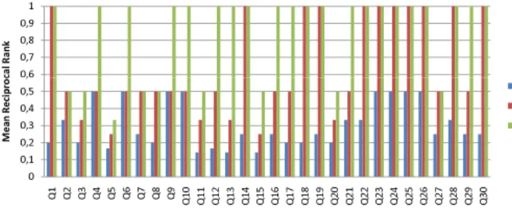
For assessing the effectiveness of the generated queries and their rankings, a standard IR metric called Reciprocal Rank (RR)defined asRR= 1/ris used, whereris the rank of the correct query. According to our problem definition, a query is correct if it matches the information need (the provided NL description). If none of the generated queries match the NL description, RR is 0. Fig. 4 shows the Mean RR (MRR, the average of the RR scores obtained from the 12 participants), which we have calculated using the scoring functionsC1,C2

andC3 as discussed in Section V.

We observe that some queries such as Q2, Q4, Q6, Q9 and Q10 get rather good results even though only the path length is used for scoring (C1). This is because the exploration results

in a low number of alternative substructures and queries, respectively. When many substructures can be found, C2

seems to be more effective as it enables the exploration to focus on more “popular” elements. Clearly, MRR obtained using C2 is at least as high as MRR obtained using C1 for

all 30 queries. However, MRR is low forC2 when ambiguity

introduced through the keyword-to-element matching is high. That is, there are many keywords that match several graph elements, such as in Q4, Q6, Q9, an Q10. Incorporating the matching relevance of keywords helps to prioritize elements that more likely match the user information need. The results show thatC3 is superior in all cases.

4_{http://tap.stanford.edu}

10000 100000

Our Solution Bidirect 1000 BFS 1000 METIS 300BFS 300METIS

1 10 100 1000 Q1 Q2 Q3 Q4 Q5 Q6 Q7 Q8 Q9 Q10

Fig. 5. Query Performance on DBLP Data.

We get similar conclusions in the evaluation with TAP, but omit them for reasons of space (see [21]).

B. Performance Evaluation

We start with a comparison with the most related ap-proaches, namely bidirectional search in [14] and several techniques based on graph indexing, i.e. 1000 BFS, 1000 METIS, 300 BFS, 300 METIS (see details in [2]).

Comparative AnalysisThe experiment is performed using the same DBLP data set and the queries as discussed in [2]. Since these approaches compute answers, we measure both the time needed for query computation and the time needed for query processing. For the latter, a prototypical RDF store called Semplore6 _{is used. Precisely, the total time is the time} for computing the top-10 queries plus the time for processing several queries (the top ones) until finding at least 10 answers. Strictly speaking, the approaches are not directly comparable. Nevertheless, since the interaction and the number of output is the same, the comparison seems reasonable.

The comparison results are shown in Fig. 5. According to these results, our approach outperforms bidirectional search by at least one order of magnitude in most cases. It also performs fairly well when compared with indexing based approaches. In particular, our approach achieves better performance when the number of keywords is large (Q7-Q10).

Search Performance We have investigated the impact of parameter k on search performance. Fig. 6a shows that the average search time (ms) for 30 queries (length 2-4) on DBLP using C3 varies at different k. It can be observed that the

time increases linearly whenkbecomes larger. In addition, the impact of query length on the search performance is minimal when kis 10. The impact of query length is substantial when a higher kis used instead.

Index Performance Since the efficiency largely depends on the size of the summary graph, we now present details on the employed indices. Fig. 6b shows that the size of the keyword index is very large for DBLP. DBLP has much more V-vertices than LUBM and TAP. This indicates that the size of the keyword index is largely determined by the number of V-vertices in the data graph. However, the size of the graph index rather depends on the structure of the data graph, the number of edge labels and classes in particular. TAP has much more classes than LUBM and DBLP, resulting in a much

6_{http://apex.sjtu.edu.cn/apex/ wiki/Demos/Semplore} Ͳ Ͳ Ͳ !""# $ % &' ( $) %

Fig. 6. a) Query Performance b) Index Performance

larger graph index. Further, the indexing time indicates that the preprocessing is affordable for practical usage.

VIII. RELATEDWORK

We have extended our previous work on keyword inter-pretation [18], [19] by proposing a concrete algorithm for top-k exploration of query graph candidates. Throughout the paper, we have discussed the most relevant related work, namely the dataguide concept [22], IR-based scoring metrics ( e.g. [15], [10], [11], [12], [8], [16]), basic search algorithms for graph exploration (in particular [2], [1], [14]) and the Threshold Algorithm [26], the fundamental algorithm for top-k

processing. We will now present a broader overview of related work on keyword search, and further information on graph exploration and top-k.

There exists a large body of work on keyword search on structured data (see [6], [1], [9], [10], [12]). Here, native approaches can be distinguished from the ones that extend existing databases with keyword search support. Native ap-proaches support keyword search on general graph-structured data. Since they operate directly on the data, these approaches have the advantage of beingschema-agnostic. However, they require specific indices and storage mechanisms ([1], [14], [2]) for the data. Database extensions require a schema, but can leverage the infrastructure provided by an underlying database. Example systems implemented as database extensions are DBXplorer [6] and Discover [9]. These systems translate keywords to candidate networks, which are essentially join expressions constructed using information given in the schema. These candidate networks are used to instantiate a number of fixed SQL queries. Our approach combines the advantages of these two approaches: in line with native approaches, it is also schema agnostic. This is crucial because even when there is a schema, it often does not capture all relations and attributes of entities (this is very frequently the case for RDF data). The summary graph is derived from the data to capture the ”schema” information that is necessary for query computation. Unlike the natives approaches, the exploration does not operate directly on the data, but on the summary graph. In addition, our approach can leverage the storage and querying capabilities of the underlying RDF store. A main difference to both the mentioned types of approaches is that, instead of comput-ing answers, we generate top-k queries. Instead of mapping keywords to data tuples, we map keywords to elements of a query. In this way, more advanced access patterns can be

supported. In particular, keywords are treated as terms in previous approaches, while they might be recognized also as query predicates in our approach. This querying capability can be further extended by introducing special elements in the summary graph that represent additional query constructs such as filters. Besides, the presentation of queries to the user can facilitate comprehension and further refinement. Also, all variable bindings are retrieved for a chosen query, instead of the roots of the top-k trees only (compare [2], [1]).

With respect tograph exploration, there are algorithms for searching substructures in tree structured data (see [24], [7], [8], [25]). More related to our work are algorithms on graphs, particularly backward search [1] and bidirectional search as discussed previously. Since the exploration of a large graph data is inherently expensive, dedicated indices are proposed to store not only keyword elements but also specific paths [8] or connectivity information of the entire graph [2]. While our approach can benefit from indexing distance information (for a more guided exploration), its application is limited to scores that can be computed off-line. The crucial difference is that while existing algorithms compute trees with distinct roots only, our search algorithm computes general subgraphs. For this, we need to traverse both incoming and outgoing edges as well as keep track of all possible distinct paths that can be used to generate subgraphs.

We have discussed that a perfectly guided exploration using pre-indexed distance information [2] can lead to results with best scores. This is however only possible with scores that can be derived from pre-indexed information. Top-k algorithms that compute scores online typically rely on TA (e.g. [1], [14], [10]). Compared to our top-kprocedure, these algorithms compute tree structures only and most importantly, rely on heuristics such that no top-k guarantee can be provided for the results.

IX. CONCLUSIONS ANDFUTUREWORK

We have presented a new approach for keyword search on graph-structured data, focusing on the RDF data model in particular. However, our algorithm is also applicable to graph-like data models in general. Instead of computing answers, novel algorithms for the top-kexploration of subgraphs have been proposed to compute queries from keywords. We have argued that it is beneficial to have an additional intermediate step in the keyword search process, where structured queries are presented to the user. Structured queries can serve as descriptions of the answers and can also be refined more precisely than using keywords. Moreover, our approach offers new ways for speeding up the process. Query computation can be performed on an aggregated graph that represents a summary of the original data while query processing can leverage optimization capabilities of the database.

In the future, techniques for indexing connectivity and scores will be considered for further speed up. Also, there is potential to advance the current query capability. For in-stance, the current indices and algorithms can be extended to

recognize keywords that correspond to special query operators such as filters etc.

REFERENCES

[1] G. Bhalotia, A. Hulgeri, C. Nakhe, S. Chakrabarti, and S. Sudarshan, “Keyword searching and browsing in databases using banks,” inICDE, 2002, pp. 431–440.

[2] H. He, H. Wang, J. Yang, and P. S. Yu, “Blinks: ranked keyword searches on graphs,” inSIGMOD Conference, 2007, pp. 305–316.

[3] K. Wilkinson, C. Sayers, H. A. Kuno, and D. Reynolds, “Efficient rdf storage and retrieval in jena2,” inSWDB, 2003, pp. 131–150. [4] E. I. Chong, S. Das, G. Eadon, and J. Srinivasan, “An efficient sql-based

rdf querying scheme,” inVLDB, 2005, pp. 1216–1227.

[5] D. J. Abadi, A. Marcus, S. Madden, and K. J. Hollenbach, “Scalable semantic web data management using vertical partitioning,” inVLDB, 2007, pp. 411–422.

[6] S. Agrawal, S. Chaudhuri, and G. Das, “Dbxplorer: enabling keyword search over relational databases,” inSIGMOD Conference, 2002, p. 627. [7] S. Cohen, J. Mamou, Y. Kanza, and Y. Sagiv, “Xsearch: A semantic

search engine for xml,” inVLDB, 2003, pp. 45–56.

[8] L. Guo, F. Shao, C. Botev, and J. Shanmugasundaram, “Xrank: Ranked keyword search over xml documents,” inSIGMOD Conference, 2003, pp. 16–27.

[9] V. Hristidis and Y. Papakonstantinou, “Discover: Keyword search in relational databases,” inVLDB, 2002, pp. 670–681.

[10] V. Hristidis, L. Gravano, and Y. Papakonstantinou, “Efficient ir-style keyword search over relational databases,” in VLDB, 2003, pp. 850– 861.

[11] H. Hwang, V. Hristidis, and Y. Papakonstantinou, “Objectrank: a system for authority-based search on databases,” inSIGMOD Conference, 2006, pp. 796–798.

[12] F. Liu, C. T. Yu, W. Meng, and A. Chowdhury, “Effective keyword search in relational databases,” inSIGMOD Conference, 2006, pp. 563– 574.

[13] B. Kimelfeld and Y. Sagiv, “Finding and approximating top-k answers in keyword proximity search,” inPODS, 2006, pp. 173–182.

[14] V. Kacholia, S. Pandit, S. Chakrabarti, S. Sudarshan, R. Desai, and H. Karambelkar, “Bidirectional expansion for keyword search on graph databases,” inVLDB, 2005, pp. 505–516.

[15] J. Graupmann, R. Schenkel, and G. Weikum, “The spheresearch engine for unified ranked retrieval of heterogeneous xml and web documents,” inVLDB, 2005, pp. 529–540.

[16] S. Amer-Yahia, N. Koudas, A. Marian, D. Srivastava, and D. Toman, “Structure and content scoring for xml,” inVLDB, 2005, pp. 361–372. [17] J. Broekstra, A. Kampman, and F. van Harmelen, “Sesame: A generic architecture for storing and querying rdf and rdf schema,” in Interna-tional Semantic Web Conference, 2002, pp. 54–68.

[18] H. Wang, K. Zhang, Q. Liu, T. Tran, and Y. Yu, “Q2semantic: A lightweight keyword interface to semantic search,” inESWC, 2008, pp. 584–598.

[19] T. Tran, P. Cimiano, S. Rudolph, and R. Studer, “Ontology-based interpretation of keywords for semantic search,” inISWC/ASWC, 2007, pp. 523–536.

[20] C. Fellbaum,WordNet, an electronic lexical database. MIT Press, 1998. [21] T. Tran, H. Wang, S. Rudolph, and P. Cimiano, “Efficient computation of formal queries from keywords on graph-structured rdf data,” in Technical Report http://www.aifb.uni-karlsruhe.de/WBS/dtr/papers/keywordTopk tr.pdf, University Karlsruhe. [22] R. Goldman and J. Widom, “Dataguides: Enabling query formulation

and optimization in semistructured databases,” inVLDB, 1997, pp. 436– 445.

[23] T. Tran, P. Cimiano, S. Rudolph, and R. Studer, “Ontology-based interpretation of keywords for semantic search,” inISWC/ASWC, 2007, pp. 523–536.

[24] D. Florescu, D. Kossmann, and I. Manolescu, “Integrating keyword search into xml query processing,” Computer Networks, vol. 33, no. 1-6, pp. 119–135, 2000.

[25] Y. Li, C. Yu, and H. V. Jagadish, “Schema-free xquery,” inVLDB, 2004, pp. 72–83.

[26] R. Fagin, A. Lotem, and M. Naor, “Optimal aggregation algorithms for middleware,” inPODS, 2001.