Online Bagging and Boosting

Online Bagging and Boosting

Nikunj

C. Oza

Intelligent Systems Division

NASA

Ames

Research Center

Mail Stop 269-3

Moffett

Field,

CA, USA

[email protected] A b s t r a c t

-

Bagging and boosting are two of the most

well-known ensemble learning methods due to their

theoretical performance guarantees and strong experimental results. However, these algorithms have been used mainly in batch mode, i.e., they require the entire training set to be available at once and, in some cases,

require random access to the data. In this paper, we

present oniine versions of bagging and boosting that require only one pass through the training data. We build

on previously presented work by presenting some

theoretical results. We also compare the online and batch algorithms experimentally in terms of accuracy and running time.

Keywords: Bagging, boosting, ensemble learning, online learning.

1 Introduction

Traditional supervised learning algorithms generate a single model such as a Na'ive Bayes classifier or multilayer perceptron (MLP) and use it to classify examples.'

Ensemble learning algorithms combine the predictions of multiple base models, each of which is l e a i e d usiiig a

traditional algorithm. Bagging [3] and Boosting [4] are well-known ensemble learning algorithms that have been shown to be very effective in improving generalization performance compared to the individual base models. Theoretical analysis of boosting's performance supports these results [4].

In previous work [ 1][2], we developed onZine versions of bagging and boosting. Online learning algorithms process each training example once "on arrival'' without the need for storage and reprocessing, and maintain a current model that reflects all the training examples seen SO far. Such algorithms have advantages over typical batch algorithms in situations where data arrive continuously. They are also u s e m with very large data sets on secondary storage, for which the multiple passes through the training set required by most batch algorithms are prohibitively expensive. In Sections 2 and 3, we describe our online bagging and online boosting algorithms, respectively. In particular, we describe how we mirror the methods that the batch bagging and boosting algorithms use to generate 1

In this paper, we only deal with the classification problem.

distinct base performance. In our preliminary

models, which are known to help ensemble previous work, we also discussed some theoretical results and some empirical comparisons of the classification accuracies of our -online algorithms and the corresponding batch algorithms on many datasets of varying size. In Sections 2 and 3, we give a brief description of some additionai theoretical resuits. in

Section 4, we review the experimental results in our previous work demonstrating the performance of our online algorithms relative to their batch counterparts. In this paper, we expand upon these results by comparing and studying their running times. We run our online bagging and boosting algorithms with two different base models: Nai've Bayes classifiers and MLPs. We use a lossless

online learning algorithm for Na'ive Bayes classifiers. For a given training set, a lossless online learning algorithm returns a model identical to that returned by the corresponding batch algorithm. For MLPs, we are forced to use a lossy online learning algorithm. In particular, we do not allow the MLP's backpropagation algorithm to cycle through the training set in multiple epochs the way backpropagation is normally allowed to do. Overall, our online bagging and boosting algorithms perform comparably to their batch counterparts in terms of classification accuracy when using Na'ive Bayes base models. The loss experienced by online MLPs relative to batch MLPs leads to a significant loss for online bagging and boosting relative to the batch versions. Online bagging often does improve significantly upon online MLPs; however, online boosting never performed sigificantly better than single online MLPs. We also compare the running times of the batch and online algorithms. If the online base model learning algorithm is not significantly slower than the corresponding batch algorithm, then the bagging and online bagging algorithms do not have a large difference in their running time in our tests. On the other hand, our online boosting algorithm runs significantly faster than batch boosting. For example, on our largest dataset, batch boosting ran twice as long as online boosting to achieve comparable classification accuracy.

2 Online Bagging

Given a training dataset T of size N , standard batch bagging creates

M

base models. Each model is trained by calling the batch learning algorithm Lb on a bootstrap sample of size N created by drawing random samples with https://ntrs.nasa.gov/search.jsp?R=20050239012 2019-08-29T21:12:30+00:00Z

replacement from the original training set. Figure 1 gives the pseudocode for bagging.

Bagging(T,Lb

>

M>

For each

rn

E

{1,2,.

.

.,

M } ,

T,

=

Sample-With-RepIacement(T,Iq)

htn = Lb(Tm)

Return

{hl,h2,.

.

.,h,}

Figure 1: Bagging Algorithm

Each base model's training set contains K copies of each of the original training examples where

N - k

P ( K

=

k )

=

(

N

)(

-Y(

1

1

-

$)

k

N

which is the Binomial distribution. As

N

+ 00, the

distribution of K tends to a Poisson(1) distribution:

P(K

=

k )

-

exp(-l)/k!.

As discussed in [ l ] [2], we can

perform bagging online as follows: as each training example d=(x,y) is presented to our algorithm, for each base model, choose the example

K

-

Poisson(1)

times and update the base model accordingly using the online base model learning algorithm Lo (see Figure 2 ) . New examples are classified the same way in online and batch bagging-by unweighted voting of the A4 base models.

OnlineBagging(h,

Lo,

d )

For each base model

h,

E

h,m

E

{1,2,.

.

. , M } .

Set

k

according to Poisson(1).

Do

k

times

Figure 2: Online Bagging Algorithm

Online bagging is a good approximation to batch bagging to the extent that their base model learning algorithms produce similar models when trained with similar distributions of training examples. In past work

[ 1 ] [ 5 ] , we proved that if the same original training set is supplied to the two bagging algorithms, then the distributions over the training sets supplied to the base models in batch and online bagging converge as the size of that original training set grows to infinity. We have also proven that the classifiers returned by bagging and online bagging converge to the same classifier given the same training set as the number of models and training examples tends to infinity under two conditions. The first is that the base model learning algorithms return classifiers that

training examples grows. The second is that, given a fixed training set T, the online and batch base model learning algorithms return the same classifier for any number of copies of T that are presented to the learning algorithm. For example, doubling the training set by repeating every example in T yields the same classifier as T would yield. For example, this condition is true of decision trees and NaYve Bayes classifiers, but is not true of MLPs, since doubling the training set effectively doubles the number of epochs in backpropagation training. More formal details are presented in [ 5 ] .

3

Online Boosting

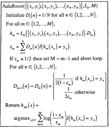
Our online boosting algorithm is designed to correspond to the batch boosting algorithm, AdaBo0st.M 1

[4] (the pseudocode is given in Figure 3). AdaBoost generates a sequence of base models

h,,

h2,.

.

.,

h,

using weighted training sets (weighted by

Dl,D2,.

.

.,OM)

such that the training examples misclassified by model

hm-l

are given half the total weight when generating model

h,

and the correctly classi.fied examples are given the remaining half of the weight. When the base model learning algorithm cannot learn with weighted training sets, one can generate samples with replacement according to

D,

AdaBoost({

(

xl,yl),(

x 2 , y 2 ) 9 * *

*,(

x N , y N ) ) , L b 9

M>

Initialize

D, ( n )

=

1

/ N

for all

n

E

{1,2,.

.

.

,

N}.

For

all

rn

E

{1,2

,...,

M } ,

N

n-1

If

E, 2

1/2

then

set

M

=

m

-

1

and

abort loop.

For all

n

E

{1,2

,...,

N } ,

Return

h,,

(x)

=

Figure 3: AdaBoost algorithm

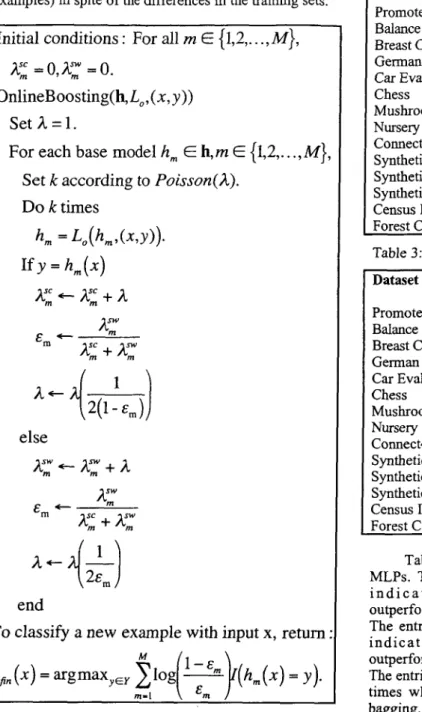
Our online boosting algorithm (Figure 4) simulates sampling with replacement using the Poisson distribution

-

when a base model misclassifies a training example, the Poisson distribution parameter

d

associated with that example is increased when presented to the next base model; otherwise it is decreased. Just as in AdaBoost, our algorithm gives the examples misclassified by one stage half the total weight in the next stage; the correctly classified examples are given the remaining half of the weight. This is done by keeping track of the total weights of each base model's correctly classified and misclassified training examples

(xi

and

a:,

respectively) and using these to update each base model's error E,,,. At this point, a

training example's weight is updated the same way as in AdaBoost.

One area of concern is that, in AdaBoost, an example's weight is adjusted based on the performance of a base model on the entire training set while in online boosting, the weight adjustment is based on the base model's performance only on the examples seen earlier. To see why this may be an issue, consider running AdaBoost and online boosting on a training set of size 10000. In AdaBoost, the first base model

h,

is trained on all 10000 examples before being tested on, say, the tenth training example. In online boosting,

h, is trained on only the first

ten examples before being tested on the tenth example. Clearly, at the moment when the tenth training example is being tested, we may expect the two

4 ' s

to be very different; therefore,

h,

in AdaBoost and

h,

in online boosting may be presented with different weights for the tenth training example. This may, in turn, lead to different weights for the tenth example when generating

h, in each

algorithm, and so on. Intuitively, we want online boosting to get a good mix of training examples so that the base models and their normalized errors in online boosting quickly converge to what they are in AdaBoost. The more rapidly this convergence occurs, the more similar the training examples' weight adjustments will be and the more similar their performances will be. We have proven [5] that for Naive Bayes base models, the online and batch boosting algorithms converge to the same ciassifier as the number of models and training examples tends to infinity.

4

Experimental Results

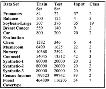
In this section, we discuss results on several different datasets, whose names and numbers of training examples, test examples, inputs, and classes are given in Table 1. The Soybean-Large and Census Income datasets come with fixed training and test sets, which we use in our experiments. For the remaining datasets, we give the training and test set sizes that result kom using 5-fold cross-validation. We discuss the results on some small datasets to show that the online algorithms can often achieve performance comparable to batch algorithms even when given a small number of data points. We discuss results on several larger datasets in more detail since online algorithms are most useful for such datasets. All but three of the datasets were drawn fiom the UCI KDD repositoq [6]. The remaining three are synthetic datasets that were

chosen because the performance of a single Naive Bayes classifier varies significantly across these three datasets. These datasets allow us to compare the performances of the online and batch ensemble algorithms on datasets of varying difficulty.

Table 1 : The datasets used in our experiments. Data Set Promoters Balance Soybean-Large Breast Cancer Car Evaluation Chess Mushroom Nursery Connect4 Synthetic-1 Synthetic-2 Synthetic-3 Census Income Forest Cnvertvne Train Set 84 500 307 559 800 1382 6499 10368 54045 80000 80000 80000 199523 464809 Test Set 22 125 3 76 140 200 346 1625 2592 13512 20000 20000 20000 99762 1 16203 Input 57 4 35' 9 20 6 22 8 42 20 20 20 39 54 Class 2 3 19 2 2 4 2 5 3 2 2 2 2 7 4.1 Accuracy

For both bagging and boosting, we present results using two' different base model types : Naive Bayes classifiers and multilayer perceptrons (MLPs). Both bagging algorithms generated 100 base models. Both boosting algorithms were allowed to generate up to 100 base models. All the results shown are based on 10 runs of 5-fold cross validation (except on the Soybean-Large and Census Income, where we used the supplied training and

test sets). A!! the o n h e algoiit,hms were r m five Piles fcr every one time the batch algorithm was run, with different random orders of the training set. This was done to account for the effect that the order of the training examples can have on the performance of an online learning algorithm.

Tables 2-5 show the results of online bagging and boosting compared to their batch counterparts and single base models using Naive Bayes classifiers and MLPs. The online MLP was trained by using backpropagation to update the MLP with each training example ten times upon arrival; however, the algorithm only ran through the entire training set once in the order in which it was presented. The batch MLP was trained by using backpropagation to update the MLP in ten epochs (ten cycles through the entire training set). All comparisons between algorithms were made using a paired t-test (a=0.05).

Table 2 shows the results of running bagging with Naive Bayes classifiers. Entries in boldfacehtalics indicate that the ensemble algorithm performed significantly bettedworse than a single Naive Bayes classifier. The bagging algorithms performed comparably to each other and mostly performed comparably to the batch Naive Bayes algorithm. This is expected due to the stability of Naive

4 0

Bayes classifiers [3]. That is, the NaYve Bayes classifiers in a bagged ensemble tend to classify new examples the same way (we obtained at least 90% agreement on all test examples) in spite of the differences in the training sets.

Initial conditions

:

For all

m

E

{1,2,.

. . ,

M},

x;

= o , q

=o.

OnlineBoosting(h,L,,(

x,

y

))

S e t d = l .

For each base model

h,

E

h,m

E

{1,2,.

.

.,

M ]

Set

k

according

to

Poisson(d).

Do

k

times

h,

=

L,(hm9(AY>).

If

y =

h,(x)

x;

-

x;

+

A

else

end

'0

classify a new

example

with

input

x,

return

Figure 4: Online Boosting Algorithm

Table 3 shows the results of running the boosting algorithms with Naive Bayes classifiers. In the (( Online Boosting )) column, any entry with a

'+'

or '-' after it indicates that online boosting performed significantly better or worse than batch boosting, respectively. Batch boosting significantly outperforms online boosting in many cases-- especially the smaller datasets. However, the performances of boosting and online boosting relative to a single Naive Bayes classifier agree to a remarkable extent. That is, when one of them is significantly better or worse than a single Naive Bayes classifier, the other tends to be the same way.

Table 2: Bagging vs. Online Bagging, Naive Bayes Dataset Naive Bagging Online Promoters 0.8774 0.8354 0.8401 Balance 0.9075 0.9067 0.9072 Breast Cancer 0.9647 0.9665 0.9661 German Credit 0.7483 0.748 0.7483 Car Evaluation 0.8569 0.8532 0.8547 Chess 0.8757 0.8759 0.8749 Mushroom 0.9966 0.9966 0.9966 Nursery 0.903 1 0.9029 0.9027 Connect4 0.7214 0.7212 0.7216 Synthetic-1 0.4998 0.4996 0.4997 Synthetic-2 0.7800 0.7801 0.7800 Synthetic-3 0.925 1 0.925 1 0.9251 Census Income 0.7630 0.7637 0.7636 Forest Covertype 0.676 1 0.6762 0.6762 Table 3: Boosting vs. Online Boosting, Naive Bayes Dataset Naive Boosting Online

Bayes Bagging Bayes Boosting Promoters 0.8774 0.8455 0.71 36- Balance 0.9075 0.8754 0.8341- German Credit 0.7483 0.735 0.68 79- Car Evaluation 0.8569 0.9017 0.8967- Chess 0.8757 0.9517 0.9476- Mushroom 0.9966 0.9999 0.9987- Nursery 0.903 1 0.9163 0.9118- Synthetic-1 0.4998 0.5068 0.5007- Synthetic-2 0.7800 0.8446 0.8376- Breast Cancer 0.9647 0.9445 0.9573+ Connect4 0.7214 0.7197 0.7209 Synthetic-3 0.925 1 0.9680 0.9688 Census Income 0.7630 0.9365 0.9398 Forest Covertype 0.676 1 0.6753 0.6753

Table 4 shows the results of running bagging with MLPs. The entries for bagging shown in boldfacehtalics i n d i c a t e t h a t b a g g i n g s i g n i f i c a n t l y outperformedhnderperformed relative to the batch MLP. The entries for online bagging shown in boldface/italics i n d i c a t e t h a t o n l i n e b a g g i n g significantly outperformedunderperformed relative to the online MLP. The entries for online bagging with a '-' after them indicate times when it performed significantly worse than batch bagging. The online MLP always performed significantly worse than the batch MLP ; therefore, it is not surprising that online bagging often performed significantly worse than batch bagging. However, online bagging did significantly outperform online MLPs most of the time.

Table 5 gives the results of running boosting with MLPs. Entries in the online MLP and boosting c o l ~ m n that are given in boldfacehtalics indicate that it significantly outperformed/underperformed relative to batch MLPs. Entries in the online boosting column given in boldfacehtalics indicate times when it significantly outperformedunderperformed relative to the online MLP.

Entries with a '-' after them indicate times when online boosting performed significantly worse

than

batch

boosting. Clearly, the significant loss in using an online MLP instead of a batch MLP has rendered the online boosting algorithm significantly worse than batch boosting.

Table 4: Bagging vs. Online Bagging, MLPs

Dataset MLP Online Bagging Online

Promoters 0.8982 0.8036 0.9036 0.7691- Balance 0.9194 0.8965 0.9210 0.9002- Breast 0.9527 0.9020 0.9561 0.8987- cancer German 0.7469 0.7062 0.7495 0.7209- Credit Evaluation MLP Bagging Car 0.9422 0.8812 0.9648 0.8877- Chess 0.9681 0.9023 0.9827 0.9185- Mushroom 1.0 0.9995 1.0 0.9988- hkiis-sery 0.9829 0.9411 0.9743 0.9390- Connect4 0.8199 0.7042 0.8399 0.7451- Synthetic-1 0.7217 0.6514 0.7326 0.6854- Synthetic-2 0.8564 0.8345 0.8584 0.8508- Synthetic-3 0.9824 0.9811 0.9824 0.9824 “ensus h o m e Zovertvne 0.9519 0.9487 0.9533 0.9487- “ ?orest 0.7573 0.6974 0.7787 0.7052- ~~~ ~ ~~

Table 5: Boosting vs. Online Boosting, MLPs

Dataset MLP Online Boosting Online

Promoters 0.8982 0.8036 0.8636 0.6155- MLP Boosting Balance 0.9194 0.8965 0.9534 0.8320- Breast 0.9527 0.9020 0.9540 0.8847- cancer German 0.7469 0.7062 0.7365 0.6788- Credit Evaluation car 0.9422 0.8812 0.9963 0.8806- Chess 0.9681 0.9023 0.9941 0.8954- Mushroom 1.0 0.9995 0.9998 0.9993- Nursery 0.9829 0.9411 0.9999 0.9445- Synthetic-1 0.7217 0.6514 0.7222 0.6344- Synthetic-2 0.8564 0.8345 0.8557 0.8117- Synthetic-3 0.9824 0.9811 0.9824 0.9583- Census 0.9519 0.9487 0.9486 0.9435 h o m e :overtype COMect4 0.8199 0.7042 0.8252 0.6807- Forest 0.7573 0.6974 0.7684 0.6329- 4.2

Running

Time

In this section, we report and analyze the running times of the batch and online algorithms that we experimented with. There are several factors that affect the difference between the running times of an online learning algorithm and its batch counterpart. Online learning algorithms’ main advantage over batch learning algorithms

is the ability to incrementally update their models with new training examples---batch algorithms often have to throw away the previously learned model and learn a new model after adding the new examples to the training set. This is clearly very wasteful computationally and is impossible when there are more data than can be stored. Additionally, batch bagging must cycle through the dataset at least MT

times, where M i s the number of base models and T is the number of times the base model learning algorithm must cycle through the training set to construct one model. Therefore, each training example is examined MT times. On

the other hand, online bagging only needs to sweep through the training set once, which means that each training example is examined only M times (once to update each base model’s parameters). Online algorithms do not require storing the entire training set. However, for a fixed training set (i.e., one to which new training examples are not continually added), batch algorithms sometimes run faster than the corresponding online algorithms. This is because batch algorithms can often set their model parameters once and for all by examining the entire training set at once while online algorithms have to update their parameters once per training example.

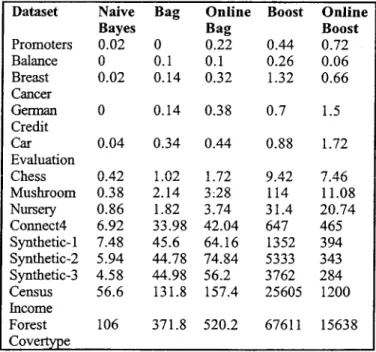
Table 6: Running times for Naive Bayes and Ensembles.

Dataset Naive Bayes Promoters 0.02 Balance 0 Breast 0.02 cancer G e m 0 Credit Car 0.04 Evaluation Chess 0.42 Mushroom 0.38 Nursery 0.86 Connect4 6.92 Synthetic-1 7.48 Synthetic-2 5.94 Synthetic-3 4.58 Census 56.6 Income Forest 106 Bag Online Bag 0 0.22 0.1 0.1 0.14 0.32 0.14 0.38 0.34 0.44 1.02 1.72 2.14 3:28 1.82 3.74 33.98 42.04 45.6 64.16 44.78 74.84 44.98 56.2 131.8 157.4 371.8 520.2 Boost Online 0.44 0.72 0.26 0.06 1.32 0.66 Boost 0.7 1.5 0.88 1.72 9.42 7.45 114 11.08 31.4 20.74 647 465 1352 394 5333 343 3762 284 25605 1200 67611 15638 Covertype

The comparison between batch and online boosting has the additional factor of the number of base models. Batch boosting, when called with the upper limit of M base models, can choose to generate fewer models---recall that if a model’s error is greater than 0.5, then boosting will discard that model and return the ensemble generated so fix. Online boosting does not have

this

luxury because it does not know what the final error rates will be for each base model. This difference can lead to lower training times for batch boosting. However, batch boosting needs to cycle through the training set M(T+I) times---each of the A4 base models requires T cycles through the training set to learn the model and one cycle to calculate the error on the

training set. Online boosting only requires one sweep through the training set.

Table 7: Running times for MLPs and Bagging.

Dataset MLP Online Bag Online

Promoters 2.58 2.34 442.7 334.6 Balance 0.12 0.14 12.48 11.7 BreastCancer 0.12 0.18 8.14 6.58 GermanCredlt 0.72 0.68 73.64 63.5 Car Evaluation 0.6 0.46 36.86 36.82 Chess 1.72 1.92 166.8 159.8 Mushroom 7.68 6.64 828.4 657.5 Nursery 9.14 9.22 1119 1005 Connect4 2338 1134 156009 105036 Synthetic- 1 142.0 149.3 15450 16056 Synthetic-2 301 124.2 24447 13328 Synthetic-3 203.8 117.5 17673 12469 Census Income 4221 1406 201489 131135 Forest Covertype 2071 805.0 126519 73902 MLP Bag

Table 8: Running times for MLP and Boosting.

Dataset MLP Online Boost Online

MLP Boost Promoters 2.58 2.34 260.9 83.18 Balance 0.12 0.14 1.96 4.18 Breast 0.12 0.18 2.56 2.28 Cancer Gellllan 0.72 0.68 11.86 23.76 Credit car 0.6 0.46 44.04 9.2 Evaluation Chess 1.72 1.92 266.7 32.42 Mushroom 7.68 6.64 91.72 53.28 Nursery 9.14 9.22 1537 160.2 Connect4 2338 1134 26461 58277 Synthetic-1 142.0 149.3 6431 8806 Synthetic-2 301 124.2 10414 5644 Synthetic3 203.8 117.5 9262 1652 Census 4221 1406 89608 52362 h o m e Forest 2071 805.0 141812 74663 :overtype

Table 6 shows the running times for Naive Bayes as vel1 as all the ensemble learning algorithms using Naive 3ayes classifiers as base models. The running time for anline bagging is generally somewhat greater than for batch bagging. The total number of times each training example is examined is the same for both batch and online bagging with Naive Bayes classifiers. However, online bagging requires a greater number of procedure calls to the learning algorithm (MT as opposed to M), which may explain the running time difference. On the other hand, online boosting has a clear running time advantage over batch boosting. Online boosting’s fewer sweeps through the dataset clearly outweigh any reduction in the number of base models returned by batch boosting. Tables 7-8 give the running times for MLPs and the batch and online ensemble

algorithms. This time, both online bagging and online boosting are faster than their batch counterparts. The batch algorithms are slowed down because each MLP requires ten cycles through the dataset.

5

Conclusions

In this paper, we discussed online versions of bagging and boosting and gave both theoretical and experimental evidence that they can perform comparably to their batch counterparts while running much faster. In this paper, we experimented only with batch datasets, i.e., one is not concerned with concept

drift.

Online algorithms are useful for batch datasets that cannot be loaded into memory in their entirety. We plan to experiment with online domains---domains where data arrive continually and where a prediction must be generated for each data point upon arrival. In these situations, the learner may be given immediate feedback (such as a calendar assistant which may suggest a meeting time which the user can either select or change) or may obtain feedback periodically. The time- varying nature of such datasets make them more difficult to deal with but more needy of online ensemble learning algorithms.

References

[ l ] Nikunj C. Oza and Stuart Russell, “Online Bagging and Boosting,” in Artificial Intelligence and Statistics 2001, Key West, FL, USA, pp. 105-1 12. January 2001. [2] Nikunj C. Oza and Stuart Russell, ‘‘Experimental Comparisons of Online and Batch Versions of Bagging and Boosting,” The Seventh ACM SIGKDD International Conference on Knowledge Discovery and Data Mining, San Francisco, CA, USA, pp. 359-364, August 2001.

[ 31 Leo Breiman, “Bagging Predictors,” Machine Learning, Vol. 24, No. 2, pp. 123-140, 1996.

[ 4 ] Yoav Freund and Robert Schapire, “A Decision- Theoretic Generalization of On-line Learning and an Application to Boosting,” Journal of Cornpurer System Sciences, Vol. 5 5 , No. 1, pp. 119-139, 1997.

[5] Nikunj C. Oza, “Online Ensemble Learning,” Ph.D. thesis, Department of Electrical Engineering and Computer Science, University of California, Berkeley, 200 1.

[ 6 ] Stephen D. Bay, “The UCI KDD Archive,” http://kdd,ics.uci.edu, Department of Information and Computer Sciences, University of California, Irvine. 1999.