The Boosted Difference of Convex Functions Algorithm for Nonsmooth Functions

THE BOOSTED DIFFERENCE OF CONVEX FUNCTIONS

ALGORITHM FOR NONSMOOTH FUNCTIONS

FRANCISCO J. ARAG ´ON ARTACHO† AND PHAN T. VUONG‡

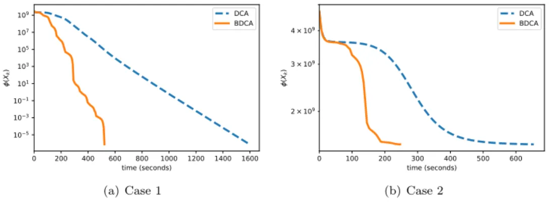
Abstract. The boosted difference of convex functions algorithm (BDCA) was recently proposed for minimizing smooth difference of convex (DC) functions. BDCA accelerates the convergence of the classical difference of convex functions algorithm (DCA) thanks to an additional line search step. The purpose of this paper is twofold. First, we show that this scheme can be generalized and successfully applied to certain types of nonsmooth DC functions, namely, those that can be expressed as the difference of a smooth function and a possibly nonsmooth one. Second, we show that there is complete freedom in the choice of the trial step size for the line search, which is something that can further improve its performance. We prove that any limit point of the BDCA iterative sequence is a critical point of the problem under consideration and that the corresponding objective value is monotonically decreasing and convergent. The global convergence and convergence rate of the iterations are obtained under the Kurdyka– Lojasiewicz property. Applications and numerical experiments for two problems in data science are presented, demonstrating that BDCA outperforms DCA. Specifically, for the minimum sum-of-squares clustering problem, BDCA was on average 16 times faster than DCA, and for the multidimensional scaling problem, BDCA was 3 times faster than DCA.

Key words. difference of convex functions, boosted difference of convex functions algorithm, Kurdyka– Lojasiewicz property, clustering problem, multidimensional scaling problem

AMS subject classifications. 65K05, 65K10, 90C26, 47N10 DOI. 10.1137/18M123339X

1. Introduction.

In this paper, we are interested in the following difference of

convex (DC) optimization problem

(

P

) minimize

x∈Rm

g(x)

−

h(x) =:

φ(x),

(1.1)

where

g

:

R

→

R

∪ {

+

∞}

and

h

:

R

→

R

∪ {

+

∞}

are proper convex functions,

with the conventions

(+

∞

)

−

(+

∞

) = +

∞

,

(+

∞

)

−

λ

= +

∞

and

λ

−

(+

∞

) =

−∞

∀

λ

∈

]

− ∞

,

+

∞

[

.

For solving (

P

), one usually applies the well-known DC algorithm (DCA) [21,

22, 34] (see section 3). DC programming and the DCA have been investigated and

developed for more than 30 years [20]. The DCA has been successfully applied in many

fields, such as machine learning, financial optimization, supply chain management,

and telecommunication [19, 22, 20]. If both functions

g

and

h

are differentiable, then

24, 2020; published electronically March 23, 2020. https://doi.org/10.1137/18M123339X

Funding:The first author was supported by MICINN of Spain and ERDF of EU, as part of the Ram´on y Cajal program (RYC-2013-13327), and the grants MTM2014-59179-C2-1-P and PGC2018-097960-B-C22. The second author was supported by the FWF (Austrian Science Fund), project M 2499-N32, and by the Vietnam National Foundation for Science and Technology Development (NAFOSTED), project 101.01-2019.320.

†_{Department of Mathematics, University of Alicante, Alicante, Spain ([email protected]).} ‡_{School of Mathematical Sciences, University of Southampton, University Road, SO17 1 BJ,}

Southampton, UK ([email protected]). 980

the boosted DC algorithm (BDCA) developed in [2] can be applied to accelerate the

convergence of DCA. Numerical experiments with various biological data sets in [2]

showed that BDCA outperforms DCA, being on average more than four times faster

in both computational time and the number of iterations. This advantage has been

also confirmed when applying BDCA to the indefinite kernel support vector machine

problem [36].

The purpose of the present paper is to develop a version of BDCA when the

func-tion

φ

is not differentiable. Unfortunatelly, when

g

is not differentiable, the direction

used by BDCA may no longer be a descent direction (see Example 3.4). For this

reason, we shall restrict ourselves to the case where

g

is assumed to be differentiable

but

h

is not. The motivation for this study comes from many applications of DC

pro-gramming where the objective function is the difference of a smooth convex function

and a nonsmooth convex function. We mention here the minimum sum-of-squares

clustering problem [13], the bilevel hierarchical clustering problem [27], the multicast

network design problem [15], and the multidimensional scaling (MDS) problem [18],

among others.

The paper is organized as follows. In section 2, we recall some basic concepts

and properties of convex analysis. As we are working with nonconvex and nonsmooth

functions, we need some tools from variational analysis for generalized differentiability.

Our main contributions are in section 3, where we propose a nonsmooth version

of the BDCA introduced in [2]. More precisely, we prove that the point generated by

the DCA provides a descent direction for the objective function at this point, even

at points where the function

h

is not differentiable. This is the key property allowing

us to employ a simple line search along the descent direction, which permits us to

achieve a larger decrease in the value of the objective function.

In section 4, we investigate the global convergence and convergence rate of the

BDCA. The convergence analysis relies on the Kurdyka– Lojasiewicz inequality. These

concepts of real algebraic geometry were introduced by Lojasiewicz [23] and Kurdyka

[16] and later developed in the nonsmooth setting by Bolte et al. [9] and Attouch

et al. [3], among many others [1, 4, 6, 8, 11, 28].

In section 5, we begin by introducing a self-adaptive strategy for choosing the trial

step size for the line search step. We show that this strategy permits us to further

improve the numerical results obtained in [2] for the above-mentioned problem arising

in biochemistry, BDCA being almost 7 times faster than DCA on average. Next,

we present an application of BDCA to two important classes of DC programming

problems in engineering: the minimum sum-of-squares clustering problem and the

MDS problem. We present some numerical experiments on large data sets, with both

real and randomly generated data, which clearly show that BDCA outperforms DCA.

Namely, on average, BDCA was 16 times faster than DCA for the minimum

sum-of-squares clustering and 3 times faster for the MDS problems. We conclude the paper

with some remarks and future research directions in the last section.

2. Preliminaries.

Throughout this paper, the inner product of two vectors

x, y

∈

R

is denoted by

h

x, y

i

, while

k · k

denotes the induced norm, defined by

k

x

k

=

p

h

x, x

i

. The closed ball of center

x

and radius

r >

0 is denoted by

B

(x, r).

2.1. Tools of convex and variational analysis.

In this subsection, we recall

some basic concepts and results of convex analysis and generalized differentiation for

nonsmooth functions, which will be used in what follows.

For an extended real-valued function

f

:

R

→

R

∪ {

+

∞}

, the domain of

f

is

the set

dom

f

=

{

x

∈

R

:

f

(x)

<

+

∞}

.

The function

f

is said to be proper if its domain is nonempty. It is said to be

convex

if

f

(

λx

+ (1

−

λ

)

y

)

≤

λf

(

x

) + (1

−

λ

)

f

(

y

)

∀

x, y

∈

R

and

λ

∈

]0

,

1[

,

and

f

is said to be

concave

if

−

f

is convex. Further,

f

is called

strongly convex

with

modulus

ρ >

0 if for all

x, y

∈

R

and

λ

∈

]0,

1[,

f

(λx

+ (1

−

λ)y)

≤

λf

(x) + (1

−

λ)f

(y)

−

1

2

ρλ(1

−

λ)

k

x

−

y

k

,

or, equivalently, when

f

−

k · k

is convex. The function

f

is said to be

coercive

if

f

(x)

→

+

∞

whenever

k

x

k →

+

∞

.

The gradient of a function

f

:

R

→

R

∪ {

+

∞}

which is differentiable at some point

x

in the interior of dom

f

is denoted by

∇

f

(

x

).

We denote by

f

(

x, d

) the one-sided directional derivative of

f

at

x

∈

dom

f

for the

direction

d

∈

R

, defined as

f

(

x

;

d

) := lim

t↓0

f

(

x

+

td

)

−

f

(

x

)

t

.

A function

F

:

R

→

R

is said to be

monotone

when

h

F

(x)

−

F

(y), x

−

y

i ≥

0

∀

x, y

∈

R

.

Further,

F

is called

strongly monotone

with modulus

ρ >

0 when

h

F

(x)

−

F

(y), x

−

y

i ≥

ρ

k

x

−

y

k

∀

x, y

∈

R

.

The function

F

is called

Lipschitz continuous

if there is some constant

L

≥

0 such

that

k

F

(x)

−

F

(y)

k ≤

L

k

x

−

y

k

∀

x, y

∈

R

,

and

F

is said to be locally Lipschitz continuous if, for every

x

in

R

, there exists a

neighborhood

U

of

x

such that

F

restricted to

U

is Lipschitz continuous.

We have the following well-known result (see, e.g., [33, Exercise 12.59]).

Fact

2.1.

A function

f

:

R

→

R

∪ {

+

∞}

is strongly convex with modulus

ρ

if

and only if

∂f

is strongly monotone with modulus

ρ

.

The

convex subdifferential

∂f

(¯

x

) of a function

f

at ¯

x

∈

R

is defined at any point

¯

x

∈

dom

f

by

∂f(¯

x) =

{

u

∈

R

|

f

(x)

−

f(¯

x)

≥ h

u, x

−

x

¯

i ∀

x

∈

R

}

and is empty otherwise.

When dealing with nonconvex and nonsmooth functions, we have to consider

subdifferentials more general than the convex one. One of the most widely used

constructions is the Clarke subdifferential, which can be defined in several (equivalent)

ways (see, e.g., [12]). For a given locally Lipschitz continuous function

f

:

R

→

R

∪ {

+

∞}

, the

Clarke subdifferential

of

f

at ¯

x

is given by

∂

f

(¯

x) = co

lim

∇

f

(x)

,

where co stands for the convex hull and Ω

denotes the set of Lebesgue measure zero

(by Rademacher’s theorem) where

f

fails to be differentiable. When

f

is also convex

on a neighborhood of ¯

x, then

∂

f

(¯

x) =

∂f(¯

x) (see [12, Proposition 2.2.7]).

Clarke subgradients are generalizations of the usual gradient of smooth functions.

Indeed, if

f

is strictly differentiable at

x, we have

∂

f

(x) =

{∇

f

(x)

}

;

see [12, Proposition 2.2.4]. However, it should be noted that if

f

is only Fr´echet

differentiable at

x, then

∂

f

(x) can contain points other than

∇

f

(x) (see, e.g., [12,

Example 2.2.3]).

The next basic formulas facilitate the calculation of the Clarke subdifferential.

Fact

2.2 (basic calculus).

The following assertions hold:

(i)

For any scalar

s

, one has

∂

(sf

)(x) =

s∂

f

(x).

(ii)

∂

(f

+g)(x)

⊂

∂

f

(x) +

∂

g(x)

, and equality holds if either

f

or

g

is strictly

differentiable.

Proof.

See [12, Propositions 2.3.1 and 2.3.3]. For the last assertion, see [12,

Corollary 1, p. 39].

2.2. Assumptions.

Throughout this paper, the following two assumptions are

made.

Assumption

1. Both functions

g

and

h

are strongly convex with modulus

ρ >

0.

Assumption

2. The function

h

is subdifferentiable at every point in dom

h, i.e.,

∂h(x)

6

=

∅

for all

x

∈

dom

h. The function

g

is continuously differentiable on an open

set containing dom

h

and

inf

x∈Rm

φ(x)

>

−∞

.

(2.1)

Under these assumptions, the next necessary optimality condition holds.

Fact

2.3 (first-order necessary optimality condition).

If

x

∈

dom

φ

is an optimal

solution of problem

(

P

)

in

(1.1)

, then

∂h(x

) =

{∇

g(x

)

}

.

(2.2)

Proof.

See [35, Theorem 3

].

Any point satisfying condition (2.2) is called a

stationary point

of (

P

). One says

that ¯

x

is a

critical point

of (

P

) if

∇

g(¯

x)

∈

∂h(¯

x).

It is obvious that every stationary point

x

is a critical point, but the converse is not

true in general.

Example

2.4. Consider the DC function

φ

:

R

→

R

defined for

x

∈

R

by

φ

(

x

) :=

k

x

k

+

X

x

−

X

|

x

.

It is not difficult to check that

φ

has 2

critical points, namely, any

x

∈ {−

1,

₀

}

,

and only one stationary point

x

:= (

−

1,

−

1, . . . ,

−

1), which is the global minimum

of

φ.

3. DCA and BDCA.

The key idea of the DCA to solve problem (

P

) in (1.1)

is to approximate the concave part

−

h

of the objective function

φ

by its affine

ma-jorization, and then minimize the resulting convex function. The algorithm proceeds

as follows.

DCA

[22]

1. Let

x

be any initial point and set

k

:= 0.

2. Select

u

∈

∂h(x

) and solve the strongly convex optimization problem

(

Pk

) minimize

x∈Rm

g(x)

− h

u

, x

i

to obtain its unique solution

y

.

3. If

y

=

x

then STOP and RETURN

x

, otherwise set

x

:=

y

, set

k

:=

k

+ 1, and go to step 2.

Let us introduce the algorithm we propose for solving problem (

P

), BDCA. The

algorithm is a nonsmooth version of the one proposed in [2], except for a small but

relevant modification in step 4, where now we give total freedom to the initial value

for the backtracking line search used for finding an appropriate value of the step size

λ

. In section 5, we demonstrate that this seemingly minor change permits

smarter

choices

of the initial value than simply using a constant value

λ. We have also replaced

λ

in the right-hand side of the line search inequality by

λ

, which allows us to remove

the inconvenient assumption

ρ > α

(see [2, Remark 3] for more details).

BDCA

1. Fix

α >

0 and 0

< β <

1. Let

x

be any initial point and set

k

:= 0.

2. Select

u

∈

∂h

(

x

) and solve the strongly convex optimization problem

(

P

) minimize

g(x)

− h

u

, x

i

to obtain its unique solution

y

.

3. Set

d

:=

y

−

x

. If

d

= 0, STOP and RETURN

x

. Otherwise, go to

step 4.

4. Choose any

λ

≥

0. Set

λ

:=

λ

.

WHILE

φ(y

+

λ

d

)

> φ(y

)

−

αλ

k

d

2

DO

λ

k

:=

βλ

.

5. Set

x

:=

y

+λ

d

. If

x

=

x

then STOP and RETURN

x

, otherwise

set

k

:=

k

+ 1, and go to step 2.

Observe that if one sets

λ

= 0, the iterations of the BDCA and the DCA coincide.

Hence, our convergence results for the BDCA apply in particular to the DCA. In the

following proposition we show that

d

:=

y

−

x

is a descent direction for

φ

at

y

.

Since the value of

φ

is always reduced at

y

with respect to that at

x

, one can achieve

a larger decrease by moving along the direction

d

. This simple fact, which is the key

idea of the BDCA, improves the performance of the DCA in many applications (see

section 5).

Proposition

3.1.

For all

k

∈

N

, the following holds:

(i)

φ(y

)

≤

φ(x

)

−

ρ

k

d

;

(ii)

φ

(y

;

d

)

≤ −

ρ

k

d

;

(iii)

there is some

δ

>

0

such that

φ

(y

+

λd

)

≤

φ(y

)

−

αλ

k

d

k

∀

λ

∈

[0, δ

],

so the backtracking step

4

of BDCA terminates finitely.

Proof.

The proof of (i) is similar to the one of [2, Proposition 3] and is therefore

omitted. To prove (ii), pick any

v

∈

∂h

(

y

). Note that the one-sided directional

derivative

φ

(

y

;

d

) is given by

φ

(y

;

d

) = lim

φ(y

+

td

)

−

φ(y

)

t

= lim

g(y

+

td

)

−

g(y

)

t

−

lim

h(y

+

td

)

−

h(y

)

t

≤ h∇

g(y

), d

i − h

v, d

i

(3.1)

by convexity of

h. Since

y

is the unique solution of the strongly convex problem

(

Pk

), we have

∇

g(y

) =

u

∈

∂h(x

).

The function

h

is strongly convex with constant

ρ. This implies, by Fact 2.1, that

∂h

is strongly monotone with constant

ρ

. Therefore, since

v

∈

∂h

(

y

), it holds that

h

u

−

v, x

−

y

i ≥

ρ

k

x

−

y

k

.

Hence

h∇

g(y

)

−

v, d

i

=

h

u

−

v, y

−

x

i ≤ −

ρ

k

d

k

,

and the proof follows by combining the last inequality with (3.1).

Finally, to prove (iii), if

d

= 0 there is nothing to prove. Otherwise, we have

lim

φ(y

+

λd

)

−

φ(y

)

λ

=

φ

(y

;

d

)

≤ −

ρ

k

d

<

−

ρ

2

k

d

<

0.

Hence, there is some

e

λ

>

0 such that

φ(y

+

λd

)

−

φ(y

)

λ

≤ −

ρ

2

k

d

∀

λ

∈

i

0,

e

λ

i

,

that is,

φ(y

+

λd

)

≤

φ(y

)

−

ρλ

2

k

d

k

∀

λ

∈

i

0,

e

λ

i

.

Setting

δ

:= min

n

e

λ

,

o

, we obtain

φ

(

y

+

λd

)

≤

φ

(

y

)

−

αλ

k

d

∀

λ

∈

]0

, δ

]

,

which completes the proof.

Remark

3.2.

(i) When the function

h

is differentiable, BDCA uses the same direction as the

Mine–Fukushima algorithm [24], since

y

+

λd

=

x

+ (1 +

λ)d

. The

algo-rithm they propose is computationally undesirable in the sense that it uses an

exact line search. This was later fixed in the Fukushima–Mine algorithm [14]

by considering an Armijo type rule for choosing the step size

x

=

x

+

β

d

=

β

y

+ 1

−

β

x

for some 0

< β <

1 and some nonnegative integer

l. Since 0

< β <

1, the

step size

λ

=

β

−

1 chosen by the Fukushima–Mine algorithm [14] is always

less than or equal to zero, while in BDCA, only step sizes

λ

∈

0, λ

are

explored. Also, the Armijo rule differs, as BDCA searches for some

λ

such

that

φ(y

+

λ

d

)

≤

φ(y

)

−

αλ

k

d

k

, while the Fukushima–Mine algorithm

requires

φ(x

+

β

d

)

≤

φ(x

)

−

αβ

k

d

k

.

(ii) We know from Proposition 3.1 that

φ

(y

+

λd

)

≤

φ(y

)

−

αλ

k

d

k

≤

φ(x

)

−

ρ

+

αλ

k

d

;

thus, BDCA results in a larger decrease in the value of

φ

at each iteration

than DCA. As a result, we can expect BDCA to converge faster than DCA.

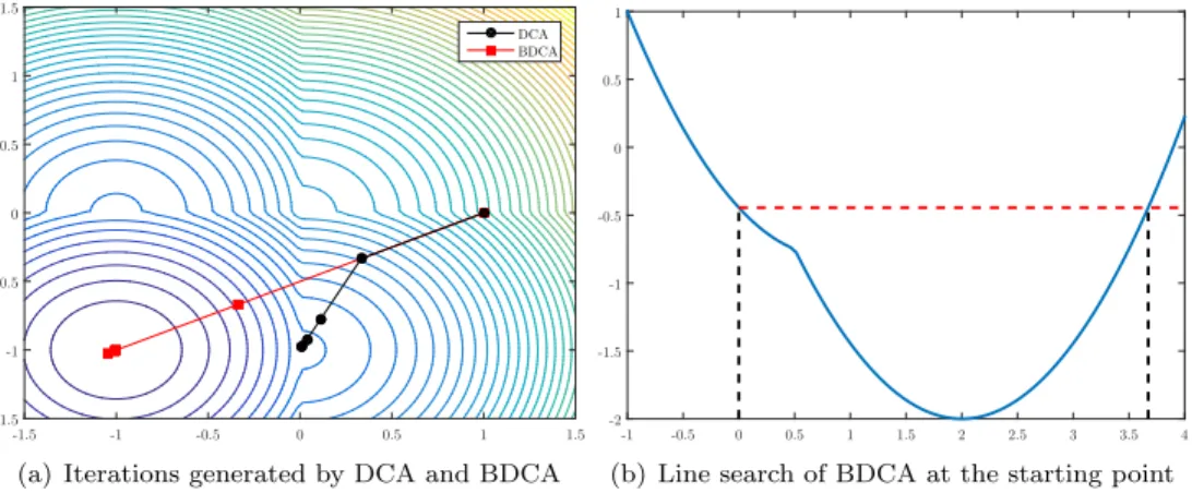
Example

3.3 (Example 2.4 revisited). Consider again the function defined in

Example 2.4 for

m

= 2. The function

φ

can be expressed as a DC function of

type (1.1) with strongly convex terms by taking, for instance,

g(x, y) =

3

2

x

+

y

+

x

+

y

and

h(x, y) =

|

x

|

+

|

y

|

+

1

2

x

+

y

.

In Figure 1(a) we show the iterations generated by DCA and BDCA from the same

starting point (x

, y

) = (1,

0), with

α

= 0.1,

β

= 0.6, and

λ

= 1 for all

k. Not only

does BDCA obtain a larger decrease than DCA in the value of

φ

at each iteration,

but also the line search helps the sequence generated escape from the stationary point

(0,

−

1), which is not even a local minimum. As the function

h

is not differentiable

at (x

, y

), there is freedom in the choice of the point in

∂h(x

, y

) =

{

2

} ×

[

−

1,

1]

(we took the point (2,

0)). In Figure 1(b) we plot the value of the function in the

line search procedure of BDCA at the first iteration. The value

λ

= 0 corresponds to

the next iteration chosen by DCA, while BDCA choses

λ >

0, which permits us to

achieve an additional decrease in the value of

φ

.

-1.5 -1 -0.5 0 0.5 1 1.5 -1.5 -1 -0.5 0 0.5 1 1.5 DCA BDCA

(a) Iterations generated by DCA and BDCA

-1 -0.5 0 0.5 1 1.5 2 2.5 3 3.5 4 -2 -1.5 -1 -0.5 0 0.5 1

(b) Line search of BDCA at the starting point

Fig. 1.Illustration of Example 3.3.

Table 1

For1million random starting points in[−1.5,1.5]2, we count the sequences generated by DCA, BDCA, the Oliveira–Tcheou algorithm (OTA)[29], and the Banert–Bot¸ algorithm (BBA)[6], con-verging to each of the four stationary points.

(−1,−1) (−1,0) (0,−1) (0,0) DCA 249,763 249,841 250,204 250,192

BDCA 1,000,000 0 0 0

OTA 1,000,000 0 0 0

BBA 250,980 249,377 249,831 249,812

Fig. 2. Comparison of the objective function value (using logarithmic scale) of DCA, BDCA,

the Oliveira–Tcheou algorithm (OTA)[29], and the Banert–Bot¸ algorithm (BBA)[6]for a particular random instance where the four algorithms converge to the global minimumx∗_{= (−1,−1).}

To demonstrate that, indeed, the line search procedure of BDCA helps the

iter-ations escape from stationary points that are not critical points, we show in Table 1

the results of running both algorithms for 1 million random starting points. For only

25% of the starting points, DCA finds the optimal solution, while BDCA finds it in

100% of the instances.

In [29], Oliveira and Tcheou have recently introduced a modification of DCA by

adding the inertial term

γ(x

−

x

) to

u

in the subproblem (

Pk

), where

γ

∈

[0,

[.

Although the sequence of objective values of the resulting algorithm is no longer

monotone, as can be observed in Figure 2, the numerical experiments in [29] show

that this term can be beneficial for escaping from stationary points that are not

critical. This is also the case here: although the scheme is slower than BDCA, the

algorithm finds the optimal solution in 100% of the instances.

Last, we test the performance of a double-proximal gradient algorithm which

was recently introduced by Banert and Bot¸ in [6]. This algorithm generates both a

primal and a dual sequence by using two proximal steps at each iteration. In our

setting, where the function

g

is smooth and its gradient is Lipschitz continuous with

constant

β

= 3, only one proximal step is needed, and the scheme reads as follows:

Let (x

, z

)

∈

R

×

R

be a pair of starting points, and set for

k

≥

0

x

=

x

+

γ

z

−

γ

∇

g(x

),

(3.2)

z

=

z

+

µ

x

−

µ

prox

µ

z

+

x

(3.3)

=

z

+

µ

x

−

µ

argmin

1

µ

h(u) +

1

2

µ

z

+

x

−

u

,

where

µ

and

γ

are some positive step sizes. To ensure that the hypotheses of the

convergence results from [6] are satisfied, we take

µ

=

γ

= 0.3

< β. We observe

in Table 1 that this algorithm also often gets stuck in stationary points. Although

the proximal step can be explicitly computed for this example, which is not always

the case and can be time-consuming, the Banert–Bot¸ algorithm turns out to be the

slowest among the three; see a particular random instance in Figure 2.

The next example complements the one given in [2, Remark 1]. It shows that the

direction used by BDCA can be an ascent direction at

y

even when this point is not

the global minimum of

φ. Thus, Proposition 3.1 does not remain valid when

g

is not

differentiable, and the scheme cannot be further extended.

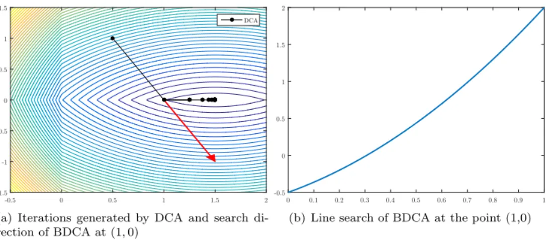
Example

3.4 (failure of BDCA when

g

is not differentiable). Consider now the

modification of the previous example

g

(

x, y

) =

−

5

2

x

+

x

+

y

+

|

x

|

+

|

y

|

and

h

(

x, y

) =

1

2

x

+

y

,

so that now

h

is differentiable but

g

is not. Let (x

, y

) = (

,

1). Then, the next point

generated by DCA is (x

, y

) = (1,

0) and

d

:= (x

, y

)

−

(x

, y

) = (

,

−

1) is not a

descent direction for

φ

at (x

, y

). Indeed, one can easily check that

φ

((x

, y

);

d

) = lim

φ

(1,

0) +

t

,

−

1

−

φ(1,

0)

t

=

3

4

;

see Figure 3. Actually, it holds that

φ

((x

, y

) +

td

)

−

φ(x

, y

) =

5t

8

+

3t

4

,

so

φ

((

x

, y

) +

td

)

> φ

(

x

, y

) for all

t >

0.

In contrast with the example in [2, Remark 1], observe that here (

x

, y

) is not

the global minimum of

φ

. In fact, the iterates generated by DCA converge to the

global minimum of

φ, as shown in Figure 3(a).

As proved next, the failure of BDCA shown in Example 3.4 can occur only

for

n

≥

2.

Proposition

3.5.

Let

φ

=

g

−

h

, where

g

:

R

→

R

and

h

:

R

→

R

are convex

and

h

is differentiable. If

h

(x)

∈

∂g(y)

and

0

6∈

∂

φ(y)

, then

φ

(y;

y

−

x)

<

0

.

Proof.

First, observe that

φ

(y;

y

−

x) = (y

−

x) sup

z∈∂g(y)

{

z

−

h

(y)

}

.

Since

h

is convex, one has

(h

(x)

−

h

(y)) (x

−

y)

≥

0.

Suppose that

x

−

y >

0. Then,

h

(x)

≥

h

(y). Since

h

(y)

6∈

∂g(y) and

∂g(y) is convex,

we deduce that

h

(y)

< z

for all

z

∈

∂g(y), which implies

φ

(y;

y

−

x)

<

0. A similar

argument shows that

φ

(y;

y

−

x)

<

0 when

x

−

y <

0. This concludes the proof.

-0.5 0 0.5 1 1.5 2 -1.5 -1 -0.5 0 0.5 1 1.5 DCA

(a) Iterations generated by DCA and search di-rection of BDCA at (1,0) 0 0.1 0.2 0.3 0.4 0.5 0.6 0.7 0.8 0.9 1 -0.5 0 0.5 1 1.5 2

(b) Line search of BDCA at the point (1,0)

Fig. 3.Illustration of Example 3.4.

We are now in a position to state our first convergence result of the iterative

sequence generated by BDCA, whose statement coincides with [2, Proposition 5].

The first part of its proof requires some small adjustments due to the nonsmoothness

of

h.

Theorem

3.6.

For any

x

∈

R

, either BDCA returns a critical point of

(

P

)

or

it generates an infinite sequence such that the following holds:

(i)

φ(x

)

is monotonically decreasing and convergent to some

φ

.

(ii)

Any limit point of

{

x

is a critical point of

(

P

)

. If in addition

φ

is coercive,

then there exists a subsequence of

{

x

}

which converges to a critical point

of

(

P

)

.

(iii)

P

k=0

k

d

k

<

+

∞

.

Further, if there is some

λ

such that

λ

≤

λ

for all

k

,

then

P

k=0

k

x

−

x

k

<

+

∞

.

Proof.

If BDCA stops at step 3 and returns

x

, then

x

=

y

. Because

y

is the

unique solution of the strongly convex problem (

Pk

), we have

∇

g(x

) =

u

∈

∂h(x

),

i.e.,

x

is a critical point of (

P

). Otherwise, by Proposition 3.1 and step 4 of BDCA,

we have

φ

(

x

)

≤

φ

(

y

)

−

αλ

k

d

k

≤

φ

(

x

)

−

αλ

+

ρ

k

d

k

.

(3.4)

Therefore, the sequence

{

φ(x

)

}

converges to some

φ

, since is monotonically

de-creasing and bounded from below by (2.1). This proves (i). As a consequence, we

obtain

φ(x

)

−

φ(x

)

→

0,

which implies

k

d

k

=

k

y

−

x

k

→

0, by (3.4).

If ¯

x

is a limit point of

{

x

}

, there exists a subsequence

{

x

}

converging to ¯

x.

Then, as

k

y

−

x

k →

0, we have

y

→

x. Since

¯

∇

g

is continuous, we get

u

=

∇

g(y

)

→ ∇

g(¯

x).

Hence, we deduce

∇

g

(¯

x

)

∈

∂h

(¯

x

), thanks to the closedness of the graph of

∂h

(see [32,

Theorem 24.4]). When

φ

is coercive, by (i), the sequence

{

x

}

must be bounded, which

implies the rest of the claim in (ii).

The proof of (iii) is similar to that of [2, Proposition 5(iii)] and is thus

omitted.

Remark

3.7. In our approach, both functions

g

and

h

are assumed to be strongly

convex with constant

ρ >

0. It is well known that the performance of DCA heavily

depends on the decomposition of the objective function [22, 31]. There is an infinite

number of ways of doing this and it is challenging to find a “good” one [31]. To get

rid of this assumption, one could add a proximal term

2

k

x

−

x

k

2

to the objective

of the convex optimization subproblem (

Pk

) in step 2, as done in the proximal point

algorithm (see [14]). This technique is employed in the proximal DCA; see [1, 6, 20, 26].

With some minor adjustments in the proofs, it is easy to show that the resulting

algorithm satisfies both Proposition 3.1 and Theorem 3.6.

4. Convergence under the Kurdyka– Lojasiewicz property.

In this

sec-tion, we prove the convergence of the sequence generated by BDCA as long as the

sequence has a cluster point at which

φ

satisfies the strong Kurdyka– Lojasiewicz

in-equality [23, 16, 9] and

∇

g

is locally Lipschitz. As we shall see, under some additional

assumptions, linear convergence can also be guaranteed.

Definition

4.1.

Let

f

:

R

→

R

be a locally Lipschitz function. We say that

f

satisfies the

strong Kurdyka– Lojasiewicz inequality

at

x

∈

R

if there exist

η

∈

]0,

+

∞

[

, a neighborhood

U

of

x

, and a concave function

ϕ

: [0, η]

→

[0,

+

∞

[

such

that

(i)

ϕ(0) = 0

;

(ii)

ϕ

is of class

C

on

]0, η[

;

(iii)

ϕ

>

₀

on

]0

, η

[

;

(iv)

for all

x

∈

U

with

f

(

x

)

< f

(

x

)

< f

(

x

) +

η

we have

ϕ

(f

(x)

−

f

(x

)) dist (0, ∂

f(x))

≥

1.

(4.1)

For strictly differentiable functions the latter reduces to the standard definition of

the Kurdyka– Lojasiewicz inequality. Bolte et al. [9, Theorem 14] show that

definable

functions

satisfy the strong Kurdyka– Lojasiewicz inequality at each point in dom

∂

f

,

which covers a large variety of practical cases.

Remark

4.2. Although the concavity of the function

ϕ

does not explicitly appear

in the statement of [9, Theorem 14], the function

ϕ

can be chosen to be concave

(since

ϕ

is o-minimal by construction, its second derivative exists and maintains the

sign on an interval ]0, δ[, and this sign is necessarily negative). If the function

f

is

not o-minimal but is convex and satisfies the Kurdyka– Lojasiewicz inequality with

a function

ϕ

which is not concave, then

f

also satisfies the Kurdyka– Lojasiewicz

inequality with another function Ψ which is concave (see [10, Theorem 29]).

Theorem

4.3.

For any

x

∈

R

, consider the sequence

{

x

}

generated by the

BDCA. Suppose that

{

x

}

has a cluster point

x

, that

∇

g

is locally Lipschitz

contin-uous around

x

, and that

φ

satisfies the strong Kurdyka– Lojasiewicz inequality at

x

.

Then

{

x

converges to

x

,

which is a critical point of

(

P

)

.

Proof.

By Theorem 3.6, we have lim

φ(x

) =

φ

.

Let

x

be a cluster point

of the sequence

{

x

}

. Then, there exists a subsequence

{

x

}

of

{

x

}

such that

lim

x

=

x

∗

. Thanks to the continuity of

φ, we deduce

φ(x

) = lim

i→+∞

φ(x

) = lim

φ(x

) =

φ

∗

.

Hence, the function

φ

is finite and has the same value

φ

at every cluster point of

{

x

.

If

φ(x

) =

φ

for some

k >

1, then

φ(x

) =

φ(x

), because the sequence

{

φ(x

)

}

is decreasing. From (3.4), we deduce that

d

= 0, so BDCA terminates after

a finite number of steps. Thus, from now on, we assume that

φ(x

)

> φ

for all

k.

Since

∇

g

is locally Lipschitz around

x

, there exist some constants

L

≥

0 and

δ

>

0 such that

k∇

g

(

x

)

− ∇

g

(

y

)

k ≤

L

k

x

−

y

k

∀

x, y

∈

B

(

x

, δ

)

.

(4.2)

Further, since

φ

satisfies the strong Kurdyka– Lojasiewicz inequality at

x

, there

exist

η

∈

]0,

+

∞

[, a neighborhood

U

of

x

, and a continuous and concave function

ϕ

: [0, η]

→

[0,

+

∞

[ such that for every

x

∈

U

with

φ(x

)

< φ(x)

< φ(x

) +

η, we

have

ϕ

(

φ

(

x

)

−

φ

(

x

)) dist (0

, ∂

φ

(

x

))

≥

1

.

(4.3)

Take

δ

small enough that

B

(x

, δ

)

⊂

U

and set

δ

:=

min

{

δ

, δ

}

. Let

K

:= max

L(1 +

λ)

αλ

+

ρ

,

(4.4)

which is attained at ˆ

λ

=

−

1 +

p

1 +

ρ/α. Since lim

x

=

x

, lim

φ(x

) =

φ

,

φ(x

)

> φ

for all

k, and

ϕ

is continuous, we can find an index

N

large enough

such that

x

∈

B

(x

, δ),

φ

< φ(x

)

< φ

+

η

(4.5)

and

k

x

−

x

k

+

Kϕ

(φ(x

)

−

φ

)

< δ.

(4.6)

By Theorem 3.6(iii), we know that

d

=

y

−

x

→

0. Then, taking a larger

N

if

needed, we can ensure that

k

y

−

x

k ≤

δ

∀

k

≥

N.

For all

k

≥

N

such that

x

∈

B

(x

, δ), we have

k

y

−

x

k ≤ k

y

−

x

+

k

x

−

x

k ≤

2δ

≤

δ

;

then, using (4.2), we obtain

k∇

g(y

)

− ∇

g(x

)

k ≤

L

k

y

−

x

=

L

1 +

λ

k

x

−

x

.

On the other hand, we have from the optimality condition of (

Pk

) that

∇

g(y

) =

u

∈

∂h(x

),

which implies, by Fact 2.2,

∇

g

(

y

)

− ∇

g

(

x

)

∈

∂h

(

x

)

− ∇

g

(

x

) =

∂

(

−

φ

(

x

)) =

−

∂

φ

(

x

)

.

(4.7)

Therefore,

dist (0, ∂

φ(x

))

≤ k∇

g(y

)

− ∇

g(x

)

k ≤

L

1 +

λ

k

x

−

x

.

(4.8)

For all

k

≥

N

such that

x

∈

B

(x

, δ) and

φ

< φ(x

)

< φ

+

η, it follows from

(4.8), the concavity of

ϕ

, (4.3), and (3.4) that

L

1 +

λ

k

x

−

x

k

(ϕ

(φ(x

)

−

φ

)

−

ϕ

(φ(x

)

−

φ

))

≥

dist (0, ∂

φ(x

)) (ϕ

(φ(x

)

−

φ

)

−

ϕ

(φ(x

)

−

φ

))

≥

dist (0, ∂

φ(x

))

ϕ

(φ(x

)

−

φ

) (φ(x

)

−

φ(x

))

≥

φ(x

)

−

φ(x

)

≥

αλ

+

ρ

k

y

−

x

k

=

αλ

+

ρ

(1 +

λ

)

k

x

−

x

k

,

which implies, by (4.4), that

k

x

−

x

k ≤

L(1 +

λ

)

αλ

+

ρ

(

ϕ

(

φ

(

x

)

−

φ

)

−

ϕ

(

φ

(

x

)

−

φ

))

≤

K

(ϕ

(φ(x

)

−

φ

)

−

ϕ

(φ(x

)

−

φ

))

.

(4.9)

We prove by induction that

x

∈

B

(x

, δ) for all

k

≥

N. Indeed, from (4.5) the

claim holds for

k

=

N

. We suppose that it also holds for

k

=

N, N

+ 1, . . . , N

+

p

−

1,

with

p

≥

1. Since

{

φ(x

)

}

is a decreasing sequence converging to

φ

, our choice

of

N

implies that

φ

< φ(x

)

< φ

+

η

for all

k

≥

N

. Then (4.9) is valid for

k

=

N, N

+ 1, . . . , N

+

p

−

1. Hence,

k

x

−

x

k ≤ k

x

−

x

k

+

X

k

x

−

x

k

≤ k

x

−

x

k

+

K

X

[ϕ

(φ(x

)

−

φ

)

−

ϕ

(φ(x

)

−

φ

)]

≤ k

x

−

x

k

+

Kϕ

(φ(x

)

−

φ

)

< δ,

where the last inequality follows from (4.6).

Thus, adding (4.9) from

k

=

N

to

P

, we get

P

X

k=N

k

x

−

x

Kϕ

(φ(x

)

−

φ

)

,

and taking the limit as

P

→

+

∞

, we conclude that

X

k=1

k

x

−

x

<

+

∞

.

(4.10)

Therefore,

{

x

is a Cauchy sequence, and since

x

is a cluster point of

{

x

}

, the

whole sequence converges to

x

. By Theorem 3.6,

x

must be a critical point

of (

P

).

Remark

4.4. In the proof of Theorem 4.3, we assume the

strong Kurdyka–

Lojasiewicz inequality

in order to have Fact 2.2(i), which allows us to deduce the

last equality in (4.7). Therefore, Theorem 4.3 remains valid if, instead of

requir-ing that

φ

satisfies the strong Kurdyka– Lojasiewicz inequality, we assume that

−

φ

satisfies the

Kurdyka– Lojasiewicz inequality

(which is defined in the same way but

replacing in (4.1) the Clarke subdifferential by the limiting subdifferential). Another

possibility would be to assume that

φ

satisfies the

symmetric Kurdyka– Lojasiewicz

inequality

, which can be defined as in Definition 4.1 with (4.1) replaced by

ϕ

(f

(x)

−

f

(x

)) dist (0, ∂

f

(x))

≥

1,

(4.11)

where

∂

f

(x) is the

symmetric subdifferential

of

f

at

x

(see, e.g., [25, p. 171]), defined

by

∂

f

(x) :=

∂

f

(x)

∪

[

−

∂

(

−

f

(x))]

,

(4.12)

with

∂

f

(

x

) denoting the

limiting subdifferential

of

f

at

x

. It is clear that

∂

f

(

x

)

⊂

∂

f

(x)

⊂

∂

f

(x) for locally Lipschitz functions. Moreover

∂

(

−

f

(x)) =

−

∂

f

(x) (see

[25, Exercise 1.75]), which is exactly what we need to deduce the last equality in (4.7).

For more information on this, we recommend the discussion in [25, pp. 61–62].

Remark

4.5. Our convergence analysis in Theorem 4.3 shares a similar flavor with

the general framework developed by Attouch, Bolte, and Svaiter in [5]. Indeed, in

that paper, the authors provided a convergence analysis for any generic algorithm for

solving nonsmooth nonconvex optimization problems satisfying two key properties:

(i) for each

k

∈

N

:

φ(x

) +

a

k

x

−

x

≤

φ(x

);

(ii) for each

k

∈

N

there exists

w

∈

∂

φ(x

) such that

k

w

k ≤

b

k

x

−

x

,

(4.13)

where

a

and

b

are some positive constants. In our convergence analysis, while we also

have the descent property (i) for BDCA (see (3.4)), it is not clear if (ii) holds. Instead

of (ii), from (4.8) we can deduce a similar property: for each

k

large enough there

exists

w

∈

∂

φ(x

) such that

k

w

b

k

x

−

x

.

(4.14)

This also opens the question of whether the general framework from Attouch, Bolte,

and Svaiter [5] still holds when we replace (4.13) by (4.14). The answer seems to be

positive, at least for DC programming.

Remark

4.6. In [28], Noll proposed an alternative algorithm for nonsmooth

non-convex optimization problems without requiring (4.13) or (4.14), where the

conver-gence analysis also heavily depends on the strong Kurdyka– Lojasiewicz inequality.

In addition, he provided an example where both (4.13) and (4.14) could fail.

An-other algorithm for DC programming whose convergence was analyzed under the

Kurdyka– Lojasiewicz inequality is the double-proximal gradient algorithm by Banert

and Bot¸ [6], which was briefly discussed in Example 3.3. This algorithm can be applied

to more general DC problems of the type

min

x∈Rm

{

g(x) +

φ(x)

−

h(Kx)

}

,

where

g

and

h

are proper, convex, and lower semicontinuous functions,

φ

is convex

and differentiable with

β

-Lipschitz continuous gradient, for some

β >

0, and

K

is

a linear mapping. Although neither strong convexity of

g

and

h, nor smoothness of

g

+φ

is required, this comes at the cost of needing to compute an additional proximal

step. Further, when

g

+

φ

is smooth, the global Lipschitz continuity of the gradient

of

φ

with a known constant is needed to guarantee the convergence of the algorithm,

because the step size is bounded above by that constant (see [6, Theorem 1]). In

contrast, only local Lipschitz continuity of

∇

g

is assumed in Theorem 4.3.

Remark

4.7. As mentioned before, if one sets

λ

= 0 for all

k, then BDCA

be-comes DCA. In this case, Theorem 4.3 is akin to [17, Theorem 3.4], where the

func-tion

φ

is assumed to be subanalytic. We also note that in this setting only one of

the functions

g

or

h

needs to be strongly convex, since one can easily check that [2,

Proposition 3] still holds, and Proposition 3.1(ii) is not needed anymore.

Next, we establish the convergence rate on the iterative sequence

{

x

}

when

φ

satisfies the strong Kurdyka– Lojasiewicz inequality with

ϕ(t) =

M t

for some

M >

0 and 0

≤

θ <

1. Observe that this property holds for all globally subanalytic

functions [9, Corollary 16], which covers many classes of functions in applications.

We will employ the following useful lemma, whose proof appears within that of [4,

Theorem 2] for specific values of

α

and

β.

Lemma

4.8 (see [2, Lemma 1]).

Let

{

s

be a nonnegative sequence in

R

and

let

α, β

be some positive constants. Suppose that

s

→

0

and that the sequence satisfies

s

≤

β

(s

−

s

)

∀

k

sufficiently large.

Then,

(i)

if

α

= 0

, the sequence

{

s

}

converges to

0

in a finite number of steps;

(ii)

if

α

∈

]0,

1]

, the sequence

{

s

}

converges linearly to

0

with rate

1

−

;

(iii)

if

α >

1

, there exists

η >

0

such that

s

≤

ηk

α−1

∀

k

sufficiently large.

Theorem

4.9.

Suppose that the sequence

{

x

generated by the BDCA has the

limit point

x

.

Assume that

∇

g

is locally Lipschitz continuous around

x

and

φ

satisfies the strong Kurdyka– Lojasiewicz inequality at

x

with

ϕ(t) =

M t

for some

M >

0

and

0

≤

θ <

1

. Then, the following convergence rates are guaranteed:

(i)

if

θ

= 0

, then the sequence

{

x

converges in a finite number of steps to

x

;

(ii)

if

θ

∈

0

,

, then the sequence

{

x

converges linearly to

x

;

(iii)

if

θ

∈

,

1

, then there exists a positive constant

η

such that

k

x

−

x

k ≤

ηk

2θ−1

for all large

k

.

Proof.

By (4.10), we know that

s

:=

P

k

x

−

x

is finite. Since

k

x

−

x

k ≤

s

by the triangle inequality, the rate of convergence of

x

to

x

can be deduced from

the convergence rate of

s

to 0.

Adding (4.9) from

i

to

P

with

N

≤

i

≤

P, we have

P

X

k=i

k

x

−

x

k ≤

Kϕ

(φ(x

)

−

φ

) =

KM

(φ(x

)

−

φ

)

,

which implies that

s

= lim

X

k

x

−

x

k ≤

KM

(φ(x

)

−

φ

)

.

(4.15)

Since

φ

satisfies the strong Kurdyka– Lojasiewicz inequality at

x

with

ϕ(t) =

M t

,

we have

M

(1

−

θ

) (

φ

(

x

)

−

φ

)

−θ

dist (0

, ∂

φ

(

x

))

≥

1

.

This and (4.8) imply

(φ(x

)

−

φ

)

≤

M

(1

−

θ) dist (0, ∂

φ(x

))

≤

M L

(1

−

θ

)

1 +

λ

k

x

−

x

≤

M L(1

−

θ)

k

x

−

x

.

(4.16)

Combining (4.15) and (4.16), we obtain

s

≤

(KM

)

(φ(x

)

−

φ

)

≤

M L(1

−

θ) (KM

)

(s

−

s

).

Applying Lemma 4.8, with

α

:=

1−θ

and

β

:=

M L(1

−

θ) (KM

)

1−θ

, we deduce the

convergence rates in (i)–(iii).

5. Applications and numerical experiments.

The purpose of this section is

to numerically compare the performance of DCA and BDCA. The lack of an explicit

form of the proximal step of the Banert–Bot¸ algorithm (3.2)–(3.3), together with the

relatively large size of our test problems, precludes the inclusion of this algorithm

in our numerical experiments. We also tested the inertial DC algorithm of Oliveira

and Tcheou [29] mentioned in Example 3.3, but we do not include any of the results

because we did not observe any difference with respect to DCA. This is due to the

small value of the inertial parameter, as it has to be set smaller than

2

to guarantee

the convergence of the algorithm, which is small in our test problems. All our codes

were written in Python 2.7 and the tests were run on an Intel Core i7-4770 CPU

3.40GHz with 32GB RAM, under Windows 10 (64-bit).

In all the experiments in this section we use the following strategy for choosing

the trial step size in step 4 of BDCA, which makes use of the previous step sizes. We

emphasize that the convergence results in the previous sections apply to any possible

choice of the trial step sizes

λ

. This is in contrast with [2], where

λ

had to be chosen

constantly equal to some fixed parameter

λ >

0.

Self-adaptive trial step size

Fix

γ >

1. Set

λ

= 0. Choose some

λ

>

0 and obtain

λ

by step 4 of BDCA.

For any

k

≥

2:

1. IF

λ

=

λ

AND

λ

=

λ

THEN set

λ

:=

γλ

; ELSE set

λ

:=

λ

.

2. Obtain

λ

from

λ

by step 4 of BDCA.

The latter

self-adaptive strategy

uses the step size that was chosen in the previous

iteration as a new trial step size for the next iteration, except in the case where two

consecutive trial step sizes were successful. In that case, the trial step size is increased

by multiplying the previously accepted step size by

γ >

1. Thus, we used a somewhat

conservative strategy in our experiments, where two successful iterations are needed

before increasing the trial step size. Other strategies could be easily considered. Since

we set

λ

= 0, the first iteration is computed with DCA. In all our experiments we

took

γ

:= 2.

The self-adaptive strategy for the trial step size has two key advantages with

respect to the

constant strategy

λ

=

λ >

0, which was used in [2]. The most

important one is that we observed in our numerical tests almost a two times speed up

in the running time of BDCA. The second advantage is that it is more adaptive and

less sensitive to a wrong choice of the parameters. Indeed, in the constant strategy,

a very large value of

λ

could make BDCA slow, due to the internal iterations needed

in the backtracking step. On the other hand, a small value of

λ

would provide a trial

step size that will be readily accepted but will result in a small advantage of BDCA

against DCA.

In the next two subsections, we compare the performance of DCA and BDCA in

two important nonsmooth problems in data analysis: the minimum sum-of-squares

clustering problem and the MDS problem. Before doing that, let us begin by

numeri-cally demonstrating that the self-adaptive strategy permits us to further improve the

results of BDCA in the smooth problem arising from the study of systems of

biochem-ical reactions tested in [2], where BDCA was shown to be more than four times faster

than DCA. To this aim, we used the same setting as in [2, section 5]. For each of

five randomly selected starting points, we obtained the 1000th iterate of BDCA with

constant trial step size strategy

λ

= 50. Next, both BDCA with self-adaptive strategy

(with

β

= 0.1) and DCA were run from the same starting point until they reached the

same objective value as the one obtained by BDCA with constant strategy. Instead

of presenting a table with the results, we show in Figure 4 the ratios of the running

times between the three algorithms, which permits us to readily compare the three

algorithms. On average, BDCA with self-adaptive strategy was 6.7 times faster than

DCA and was 1.7 times faster than BDCA with constant strategy, which in turn was

4.2 times faster than DCA.

Fig. 4. Ratios of the running times of DCA, BDCA with constant trial step size and BDCA

with self-adaptive trial step size for finding a steady state of various biochemical reaction network models [2]. For each of the models, the algorithms were run using the same five random starting points. The average is represented with a dashed line.

In the next two subsections we present various experiments with problems in data

analysis. We consider two types of data: real and random. As real data, we use the

geographic coordinates of the Spanish cities with more than 500 habitants.

The

advantage of this relatively large data in

R

is that it permits us to visually illustrate

some of the experiments.

5.1. The minimum sum-of-squares clustering problem.

Clustering is an

unsupervised technique for data analysis whose objective is to group a collection of

objects into clusters based on similarity. This is among the most popular techniques

in data mining and can be mathematically described as follows. Let

A

=

{

a

, . . . , a

}

be a finite set of points in

R

, which represent the data points to be grouped. The

goal is to partition

A

into

k

disjoint subsets

A

, . . . , A

, called clusters, such that a

clustering criterion is optimized.

There are many different criteria for the clustering problem. One of the most used

is the

minimum sum-of-squares clustering

criterion, where one tries to minimize the

Euclidean distance of each data point to the centroid of its cluster [7, 13, 30]. Thus,

each cluster

A

is identified by its center (or centroid)

x

∈

R

, j

= 1, . . . , k. Letting

X

:=

x

, . . . , x

∈

R

, this gives rise to the following optimization problem:

minimize

ϕ(X, ω) :=

1

n

X

X

ω

k

x

−

a

k

,

where the binary variables

ω

express the assignment of the point

a

to the cluster

j,

i.e.,

ω

= 1 if

a

∈

A

, and

ω

= 0 otherwise. This problem can be equivalently

refor-mulated as the following nonsmooth nonconvex unconstrained optimization problem

(see [13, 30]):

minimize

φ(X) :=

1

n

X

min

k

x

−

a

k

.

(5.1)

As explained in [13, 30], we can write this problem as a DC problem of type (1.1) by

taking

g

(

X

) :=

1

n

X

X

x

−

a

+

ρ

2

k

X

k

,

h(X) :=

1

n

X

max

X

x

−

a

+

ρ

2

k

X

k

,

for some

ρ

≥

0, where

k

X

k

is the Frobenius norm of

X

. Observe that both functions

g

and

h

are convex, and strongly convex if

ρ >

0. Moreover,

g

is differentiable,

and the subdifferential of

h

can be explicitly computed (see [30, p. 346] or [13,

equation (3.21)]).

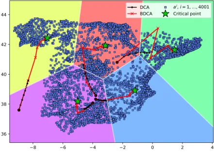
Experiment

5.1 (clustering the Spanish cities in the peninsula).

Consider the

problem of finding a partition into five clusters of the

4001

Spanish cities in the

penin-sula with more than

500

residents. For illustrating the difference between the iterations

of DCA and BDCA, we present in Figure

5

the result of applying

7

iterations of DCA

1_{The data can be retrieved from the Spanish National Center of Geographic Information at} http://centrodedescargas.cnig.es.

Fig. 5. Seven iterations of DCA and BDCA are computed from the same starting point for grouping the Spanish cities in the peninsula into five clusters.

and BDCA to the clustering problem

(5.1)

from a random starting point (composed by

a quintet of points in

R

), with the parameters

ρ

=

,

α

= 0.1

,

β

= 0.5

, and

λ

= 5

.

Both algorithms converge to the same critical point, but it is apparent that the line

search of BDCA makes it faster.

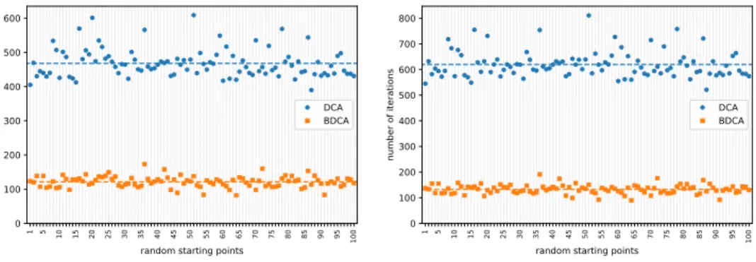
Let us demonstrate that the behavior shown in Figure

5

is not atypical. To do

so, let us consider the same problem of the Spanish cities for a different number of

clusters

k

∈ {

5,

10,

15,

20,

25,

50,

75,

100

}

. For each of these values, we run BDCA

for

100

random starting points with coordinates in

]

−

9.26,

3.27[

×

]36.02,

43.74[

(the

range of the geographical coordinates of the cities). The algorithm was stopped when

the relative error of the objective function

φ

was smaller than

10

. Then, DCA was

run from the same starting point until the same value of the objective function was

reached, which did not happen in

31

instances because DCA

failed

(by which we mean

that it converged to a worse critical point). In Figure

6

we have plotted the ratios

between the running time and the number of iterations, except for those instances

where DCA failed. On average, BDCA was

16

times faster than DCA, and DCA

needed

18

times more iterations to reach the same objective value as BDCA.

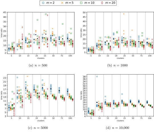
Experiment

5.2 (clustering random points in an

m

-dimensional box).

In this

numerical experiment, we generated

n

random points in

R

whose coordinates were

drawn from a normal distribution having a mean of

0

and a standard deviation of

10

, with

n

∈ {

500,

1000,

5000,

10,000

}

and

m

∈ {

2,

5,

10,

20

}

. For each pair of values

of

n

and

m

,

10

random starting points were chosen and BDCA was run to solve the

k

-clustering problem until the relative error of the objective function was smaller than

10

, with

k

∈ {

5,

10,

15,

20,

25,

50,

75,

100

}

. As in Experiment

5.1

, we run DCA from

the same starting point as BDCA until the same value of the objective function was

reached. The DCA failed to do so in

123

instances. The ratios between the respective

running times are shown in Figure

7

. On average, BDCA was

13.7

times faster than

DCA.

Fig. 6.Comparison between DCA and BDCA for solving the clustering problem of the cities in the Spanish peninsula described in Experiment 5.1. We represent the ratios of running time (left) and number of iterations (right) between DCA and BDCA for100random instances for different values of the number of clustersk∈ {5,10,15,20,25,50,75,100}. The dashed line shows the overall average ratio, and the red dots represent the average ratio for each value ofk.

(a)n= 500 (b)n= 1000

(c)n= 5000 (d)n= 10,000

Fig. 7. Comparison between DCA and BDCA for solving the clustering problems with

ran-dom data described in Experiment 5.2. For each value of n ∈ {500,1000,5000,10,000} and

m ∈ {2,5,10,20} we represent the ratios of running time between DCA and BDCA for 10 ran-dom starting points for