Towards Automatic Machine Learning Pipeline Design

UC Berkeley Electronic Theses and Dissertations

Title

Towards Automatic Machine Learning Pipeline Design Permalink https://escholarship.org/uc/item/2163j1c4 Author Milutinovic, Mitar Publication Date 2019 Peer reviewed|Thesis/dissertation

eScholarship.org Powered by the California Digital Library

by

Mitar Milutinovic

A dissertation submitted in partial satisfaction of the requirements for the degree of

Doctor of Philosophy in Computer Science in the Graduate Division of the

University of California, Berkeley

Committee in charge: Professor Dawn Song, Chair

Professor Trevor Darell Professor Joseph Gonzalez

Professor James Holston

Copyright 2019 by Mitar Milutinovic

This work is licensed under the Creative Commons Attribution-ShareAlike 4.0 International License

To view a copy of this license, visit

Abstract

Towards Automatic Machine Learning Pipeline Design by

Mitar Milutinovic

Doctor of Philosophy in Computer Science University of California, Berkeley

Professor Dawn Song, Chair

The rapid increase in the amount of data collected is quickly shifting the bottleneck of making informed decisions from a lack of data to a lack of data scientists to help analyze the collected data. Moreover, the publishing rate of new potential solutions and approaches for data analysis has surpassed what a human data scientist can follow. At the same time, we observe that many tasks a data scientist performs during analysis could be automated. Automatic machine learning (AutoML) research and solutions attempt to automate portions or even the entire data analysis process.

We address two challenges in AutoML research: first, how to represent ML programs suitably for metalearning; and second, how to improve evaluations of AutoML systems to be able to compare approaches, not just predictions.

To this end, we have designed and implemented a framework for ML programs which provides all the components needed to describe ML programs in a standard way. The frame-work is extensible and frameframe-work’s components are decoupled from each other, e.g., the framework can be used to describe ML programs which use neural networks. We provide reference tooling for execution of programs described in the framework. We have also de-signed and implemented a service, a metalearning database, that stores information about executed ML programs generated by different AutoML systems.

We evaluate our framework by measuring the computational overhead of using the frame-work as compared to executing ML programs which directly call underlying libraries. We observe that the framework’s ML program execution time is an order of magnitude slower and its memory usage is twice that of ML programs which do not use this framework.

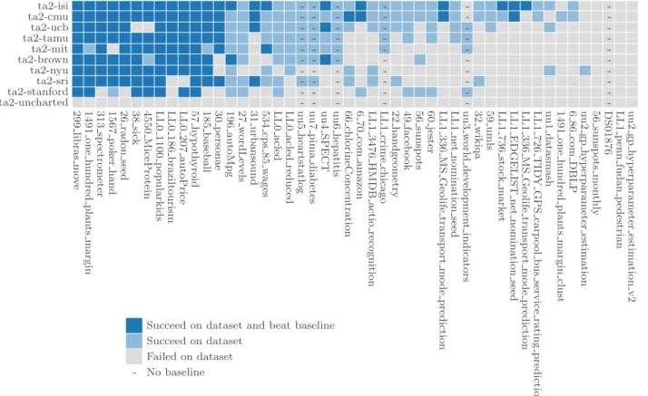
We demonstrate our framework’s ability to evaluate AutoML systems by comparing 10 different AutoML systems that use our framework. The results show that the framework can be used both to describe a diverse set of ML programs and to determine unambiguously which AutoML system produced the best ML programs. In many cases, the produced ML programs outperformed ML programs made by human experts.

Contents

3.7 Basic data types . . . 22

3.8 Data references . . . 23 3.9 Metadata . . . 23 3.10 Execution semantics . . . 26 3.11 Example pipeline . . . 29 3.12 Problem description . . . 31 3.13 Reference runtime . . . 33 3.14 Evaluating pipelines . . . 33 3.15 Metalearning . . . 34 4 Pipelines in practice 35 4.1 Standard pipelines . . . 35 4.2 Linear pipelines . . . 36 4.3 Reproducibility of pipelines . . . 40

4.5 Overhead . . . 44

4.6 Use in AutoML systems . . . 45

5 Future work and conclusions 48 5.1 Evaluating pipelines on raw data . . . 48

5.2 Simplistic problem description . . . 49

5.3 Data metafeatures . . . 49

5.4 Pipeline metafeatures . . . 49

5.5 Pipeline validation . . . 50

5.6 Pipeline execution optimization . . . 50

5.7 Conclusions . . . 51 A Terminology 53 B Pipeline description 55 C Problem description 56 D Primitive metadata 58 E Container metadata 60 F Data metadata 62 G Semantic types 64

H Hyper-parameter base classes 70

I Pipeline run description 73

J Example pipeline 75

K Example linear pipeline 80

L Example neural network pipeline 83

List of Figures

1.1 Annual size of the global datasphere . . . 1

1.2 Number of AI/ML preprints on arXiv published each year . . . 2

3.1 Example ML program in Python programming language . . . 9

3.2 Example program in a different programming style . . . 10

3.3 Example hyper-parameters configuration . . . 21

3.4 Visual representation of example metadata selectors . . . 25

3.5 Visual representation of an example pipeline . . . 30

3.6 Visual representation of the example pipeline with all hyper-parameter values . 32 4.1 Conceptual representation of a general pipeline . . . 35

4.2 Conceptual representation of a standard pipeline . . . 36

4.3 Conceptual representation of a linear pipeline . . . 36

4.4 Visual representation of an example linear pipeline . . . 37

4.5 Visual representation of an example pipeline of a neural network . . . 43

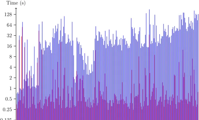
4.6 Averaged execution times of ML programs and corresponding pipelines . . . 46

List of Tables

1.1 The intensification of local shortages for data science skills . . . 2

1.2 A sample of the Iris dataset . . . 4

1.3 An example metalearning dataset . . . 4

Acknowledgments

Foremost, I would like to thank my wife Andrea and my son Nemo for their utmost patience. All your hugs gave me all the energy I needed.

In no particular order, I would like to thank Ryans Zhuang, Kevin Zeng, Julia Cao, Roman Vainshtein, Rok Mihevc, Asi Messica, Charles Packer, and many other colleagues and students at UC Berkeley with whom I have worked on projects and research underpinning this work. Without you this work would not have been possible.

This work builds on many other projects and collaborations, primarily through the Darpa D3M program. I would like to thank everyone in the program, and especially those active in working groups through which discussed many topics present in this work. Just to name a few who have again and again stepped up to various challenges along the way: Diego Martinez, Brandon Schoenfeld, Sujen Shah, Mark Hoffmann, Alice Yepremyan, Shelly Stanley. No list would be complete without Wade Shen, who has had the vision and commitment to push the program through despite all the issues along the way. Moreover, Rob Zinkov, Atılım G¨une¸s Baydin, and Frank Wood were pivotal in pushing me to see that what has been a simple initial straw man proposal can be much more, and that has ultimately led to this work.

Amazing Ray team, especially Robert Nishihara and Richard Liaw, thank you for guiding me when I got stuck. Moreover, thank you for addressing issues and feature requests quickly and efficiently, this makes your project really special.

Thank you to all who read through early drafts of this work and gave valuable feedback, especially Diego Martinez, Brandon Schoenfeld, Adrianne Zhong, Marten Lohstroh, and Andreas Mueller.

I was lucky to have not just one but three advisors: professors Dawn Song, Trevor Darell, and Joseph Gonzalez. Thank you for all the insights, suggestions, hard questions, and gentle pushes. Each of you contributed a fundamental piece of my experience at UC Berkeley.

Of course, without my parents and their support at every step along the way, nothing would have ever been possible. Thank you.

Chapter 1

Introduction

Figure 1.1: Annual size of the global datasphere. Source: IDC, November 2018, sponsored by Seagate [39].

Data available for potential use in ML programs is growing at a high rate as shown in Figure 1.1. IDC forecasts the global datasphere to grow to 50 ZB by 2020 [39]. At the same time there is a shortage of data scientists, Table 1.1. Looking at the number of AI/ML preprints on arXiv in cs.AI, stat.ML, and cs.NE categories published each year (Figure 1.2) we can see that it is growing dramatically and that just in 2018 there were more than 12,000 preprints published on arXiv alone. Those preprints can contain potential new solutions and approaches which could be used in ML programs. But it is not possible for any single individual to learn about them all, to learn for which problems and data types they are useful, to learn their effective combinations, nor how they could be used in ML programs.

One way to address this challenge is by using an Automated Machine Learning (AutoML) system to help analyze data and build ML programs which use data. Given data and a

Metro Area July 2015 July 2018 3Y Delta New York City, NY +4,132 +34,032 +29,900 San Francisco Bay Area, CA +10,995 +31,798 +20,803 Los Angeles, CA +425 +12,251 +11,826 Boston, MA +1,667 +11,276 +9,609 Seattle, WA +1,182 +9,688 +8,506 Chicago, IL −1,826 +5,925 +7,751 Washington, D.C. +735 +7,686 +6,951 Dallas-Ft. Worth, TX −2,496 +3,641 +6,137 Atlanta, GA −2,301 +3,350 +5,651 Austin, TX +26 +4,949 +4,923

Table 1.1: The intensification of local shortages for data science skills, July 2015 to July 2018. Table provides the shortage (+) or surplus (-) of people with data science skills in each metro area, and the associated delta over three years. Source: LinkedIn [26].

0 2,000 4,000 6,000 8,000 10,000 12,000 Preprints 1994 1996 1998 2000 2002 2004 2006 2008 2010 2012 2014 2016 2018 Year Figure 1.2: Number of AI/ML preprints on arXiv in cs.AI, stat.ML, and cs.NE categories published each year. Source: arXiv, May 2019 [8].

problem description, an AutoML system automatically creates an ML program to preprocess this data and to build a machine learning model solving the problem. Ideally, the automatic process of creation of an ML program should take into account all existing ML knowledge.

In the context of AutoML research, there are two challenges we tackle in this work: how to compare AutoML systems and how to better support AutoML systems which use metalearning.

Comparison of AutoML systems

There are many attempts at AutoML systems both in academia and industry (see Chap-ter 2), but there are many challenges to deChap-termine the quality of those AutoML systems.‘ Quality of an AutoML system can consist of many factors, e.g.:

• How much resources it needs to run?

• How quickly it creates an ML program?

• How far is this ML program from the best ML program?

• How clean or structured input data has to be?

• Which problem types does it support?

• How well it searches the space of possible ML programs?

Moreover, comparison of AutoML systems is hard because they use different sets of building blocks in their ML programs and use different datasets for their reported evaluation. If building blocks are different, maybe one AutoML system has simply a better building block available and this is why its ML program outperforms an ML program made by some other AutoML system. But if both systems used the same building blocks, it might be the case that the latter AutoML system creates that same (better) ML program as well and even faster.

Furthermore, it is hard to compare AutoML systems if the quality of ML programs themselves is not well defined or if different ML programs use different definitions of qual-ity. Generally we care about ML program’s quality of predictions as computed by some metric, but there are also other aspects of ML programs we can care about: complexity, interpretability, generalizability, resources and data requirements, etc.

Metalearning

One big family of approaches to AutoML is centered around metalearning. Metalearning treats AutoML itself as an ML problem. Because both ML programs as created by such an AutoML system and the AutoML system itself both operate on data and build an ML

sepal length sepal width petal length petal width species 5.1 3.5 1.4 0.2 Iris-setosa 4.9 3 1.4 0.2 Iris-setosa 7 3.2 4.7 1.4 Iris-versicolor 6.4 3.2 4.5 1.5 Iris-versicolor 6.3 3.3 6 2.5 Iris-virginica 5.8 2.7 5.1 1.9 Iris-virginica

Table 1.2: A sample of the Iris dataset [2, 15]. dataset problem description program ID score iris classification ca41e6a5 0.87 iris classification 759e40f2 0.93

boston regression 8727d30d 0.85

boston regression 3ad4cc03 0.99

sunspots forecasting 37181a32 0.91 sunspots forecasting e863382f 0.51

Table 1.3: An example metalearning dataset.

model, we use prefix meta when talking about the data and model of an AutoML system which uses metalearning: metalearning dataset or meta-dataset and meta-model.

For metalearning a dataset is needed which serves as input to a meta-model. If a regular tabular dataset looks like Table 1.2, a metalearning dataset looks like Table 1.3: instead of samples with attributes and targets, each sample consists, conceptually, of a dataset, a problem description, a program, and a score achieved by executing the program on the dataset and the problem description. A meta-model is trained that for a given new dataset and a problem description it constructs an ML program which achieves the best score. There are many challenges about metalearning, but in this work we focus on how to represent programs in such metalearning dataset. Representation of datasets and problem descriptions we leave to future work in Sections 5.2 and 5.3.

1.1

Contributions

We address challenges presented with the following contributions:

• We have designed and implemented a framework for ML programs which provides all components needed to describe ML programs in a standard way suitable for metalearn-ing. The framework is extensible and framework’s components are decoupled from each other.

• We present how this framework is used by 10 AutoML systems and how it addresses the challenge of comparison of AutoML systems.

• We have designed and implemented a service to serve as a metalearning dataset, storing information about executed ML programs by different AutoML systems.

Contributions empower each other: a standard way of describing ML programs enables both better comparison between AutoML systems and metalearning across ML programs created by different AutoML systems, allowing shared representation of information about executed ML programs and construction of a metalearning dataset.

Chapter 2

Related work

The AutoML research field is active and vibrant and has produced many academic and non-academic systems [10, 14, 18, 20, 22, 23, 27, 28, 31, 32, 38, 40, 41, 42, 43, 45, 47, 50, 52], including some focusing on neural networks only [3, 9, 21, 29, 36, 53]. Wse can observe [12] that there are many approaches they take and that they are implemented in various pro-gramming languages. Those differences lead to challenges in comparison of AutoML systems. Existing comparisons [17, 19] compare only predictions made by those systems. While for practical purposes it is important to compare what can systems achieve as they are, it does not provide any insight into how well the approaches they are taking fundamentally com-pare. Comparison is further complicated because different systems support different data types and task types. In this work we present a framework which enables comparison of approaches and not just predictions, across data types and problem types.

Many AutoML systems, to our knowledge at least [10, 14, 27, 40, 41, 43, 52], use some sort of metalearning. But they cannot learn from results across systems. Our framework addresses that through shared representation of ML programs and a shared metalearning service. [49] is a similar shared service to store information about ML programs and their performance on various datasets, but stored performance scores are self-reported and ML programs are not necessarily reproducible, limiting usefulness for cross-system metalearning. Systems which focus on neural networks [3, 9, 21, 29, 36, 53] can be combined with other AutoML systems using our framework.

AutoML systems do not use one shared representation of ML programs. There are some popular pipeline languages which might be candidates for such a purpose. scikit-learn [33] pipeline allows combining multiple scikit-scikit-learn transforms and estimators. While powerful, it inherits some weaknesses from scikit-learn itself, primarily its support for only tabular and already structured data. This prevents it to be used when inputs are raw files. Moreover, its combination of linear and nested structure can become very verbose. Common Workflow Language [46] is a standard for describing data-analysis workflows with focus on reproducibility. But its focus is also on combining command line programs into workflows, which is generally not what ML programs made by AutoML systems consist of. Kubeflow [24] provides a pipeline language and at the same time makes their deployments on Kubernetes

simple. Similar to our framework it allows combining components using different libraries, but every component is a Docker image, and instead of directly passing memory objects between components, inputs and outputs have to be serialized.

There are existing tools to describe hyper-parameters configuration [5, 13]. Our frame-work aims to be compatible with them while extending a static configuration with optional custom sampling logic. This allows authors to define a new type of a hyper-parameter space and provide a custom sampling logic without AutoML systems having to support that type of a hyper-parameter space in advance.

Chapter 3

Framework for ML pipelines

We have designed and implemented a framework for ML programs for use in AutoML systems. We provide reference tooling for execution of programs described as framework’s

pipelines. We have designed and implemented a service to store and share information about

executed pipelines as pipeline run descriptions. The collection of pipeline run descriptions can serve as a metalearning dataset.

In this chapter we present technical details of the framework and related tooling and service.

3.1

Design goals

In 2019, the most popular programming language for ML programs was Python [11]. An example of such an ML program in Python for the Thyroid disease dataset [48] is available in Figure 3.1. In the example program we first select a target column and attribute columns from input data. Then we further select numerical and categorical attributes. We encode categorical attributes and we impute missing values in numerical attributes. After that we combine categorical attributes and numerical attributes back into one data structure of all attributes. We then pass this data structure, together with targets, to a classifier to fit and predict. The program runs in two passes, in the first we fit on training data and in the second pass we only predict on testing data. This example program contains general steps found in ML programs: data loading, data selection and cleaning, and finally model building. It does not contain common steps like feature extraction, construction, and selection.

If we look at such ML programs as raw input of an AutoML system from which the system might want to learn from, we can observe:

• Language specific constructs which have nothing to do with the ML task at hand, e.g.,

import statements.

• Syntax of the programming language allows logically equivalent programs to be repre-sented with different characters (changing a variable name does not change the logic

1 import numpy

2 import pandas

3 from sklearn.preprocessing import OrdinalEncoder

4 from sklearn.impute import SimpleImputer

5 from sklearn.ensemble import RandomForestClassifier

6 7 train_dataframe = pandas.read_csv(’sick_train_split.csv’) 8 test_dataframe = pandas.read_csv(’sick_test_split.csv’) 9 10 encoder = OrdinalEncoder() 11 imputer = SimpleImputer() 12 classifier = RandomForestClassifier(random_state=0) 13

14 def one_pass(dataframe, is_train):

15 target = dataframe.iloc[:, 30] 16 attributes = dataframe.iloc[:, 1:30] 17 18 numerical_attributes = attributes.select_dtypes(numpy.number) 19 categorical_attributes = attributes.select_dtypes(numpy.object) 20 21 categorical_attributes = categorical_attributes.fillna(’’) 22 23 if is_train: 24 encoder.fit(categorical_attributes) 25 imputer.fit(numerical_attributes) 26 27 categorical_attributes = encoder.transform(categorical_attributes) 28 numerical_attributes = imputer.transform(numerical_attributes) 29 30 attributes = numpy.concatenate([ 31 categorical_attributes, 32 numerical_attributes, 33 ], axis=1) 34 35 if is_train: 36 classifier.fit(attributes, target) 37 38 return classifier.predict(attributes) 39 40 one_pass(train_dataframe, True)

41 predictions = one_pass(test_dataframe, False)

1 import numpy

2 import pandas

3 from sklearn.compose import make_column_transformer

4 from sklearn.pipeline import make_pipeline

5 from sklearn.preprocessing import OrdinalEncoder

6 from sklearn.impute import SimpleImputer

7 from sklearn.ensemble import RandomForestClassifier

8 9 train_dataframe = pandas.read_csv(’sick_train_split.csv’) 10 test_dataframe = pandas.read_csv(’sick_test_split.csv’) 11 12 train_attributes = train_dataframe.iloc[:, 1:30] 13 train_target = train_dataframe.iloc[:, 30] 14 test_attributes = test_dataframe.iloc[:, 1:30] 15 16 def get_numerical_attributes(X):

17 return X.dtypes.apply(lambda d: issubclass(d.type, numpy.number))

18

19 def get_categorical_attributes(X):

20 return X.dtypes == ’object’

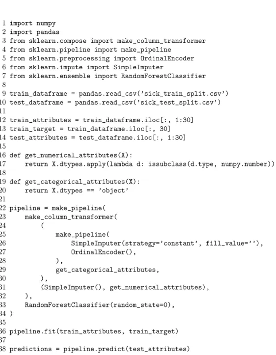
21 22 pipeline = make_pipeline( 23 make_column_transformer( 24 ( 25 make_pipeline( 26 SimpleImputer(strategy=’constant’, fill_value=’’), 27 OrdinalEncoder(), 28 ), 29 get_categorical_attributes, 30 ), 31 (SimpleImputer(), get_numerical_attributes), 32 ), 33 RandomForestClassifier(random_state=0), 34 ) 35 36 pipeline.fit(train_attributes, train_target) 37 38 predictions = pipeline.predict(test_attributes)

of the program, adding a comment or empty lines neither).

• Different programming styles might lead to very different programs and different ways of expressing the same underlying logic. The program in Figure 3.2 uses a different programming style, but is logically equivalent to the program in Figure 3.1.

• The programming language used is a general programming language which allows pro-gram to do more than just solve an ML task, e.g., display user interface, periodically save state, parallelize execution. That code is interleaved with code corresponding to the ML task.

• The programming language allows code with side effects and non-determinism. This can lead to a program not producing the same results when run multiple times on the same input data. Reproducibility of results can be achieved primarily through programming discipline.

Such properties of a programming language and programs in that language are gen-erally reasonable and even seen as an advantage of the programming language when the programming language is used by humans. But in the context of AutoML systems which would consume such programs for learning and produce new programs as their outputs, all automatically, those properties can be seen as unnecessary complexity.

In this work we present a framework for ML pipelines that AutoML systems can directly consume and produce. The design goals of this framework are:

• The framework should allow most of ML and data processing programs to be described as its pipelines, if not all, but be as simple as possible to facilitate both automatic generation and automatic consumption of pipelines.

• Pipelines should allow description of complete end-to-end ML programs, starting with raw files and finishing with predictions or any other ML output from models embedded in pipelines.

• The focus of the framework is machine generation and consumption as opposed to human generation and consumption. It should enable automation as much as possible.

• The framework should be extensible and framework’s components should be decoupled from each other, cf. in most programming languages a typing system and execution semantics are tightly coupled with the language itself.

• Control of side-effects and randomness in pipelines, and in general full reproducibility should be part of the framework and not an afterthought.

3.2

Syntax of pipelines

Pipelines do not have a human-friendly syntax and are primarily represented as in-memory data structures. Many of our framework’s components, including pipelines, can be represented in JSON [6] or YAML [4] serialization formats. We provide validators using JSON Schema [16] to validate serialized data structures.

3.3

Pipeline structure

In our framework, ML programs are described as pipelines. Such pipelines consist of:

• Pipeline metadata.

• Specification of inputs and outputs of the pipeline.

• Definition of pipeline steps.

While pipeline is an in-memory structure, we call its standard representation a pipeline

description. We support JSON and YAML serialization formats for pipeline descriptions

and we provide a validator for pipeline descriptions using JSON Schema. The full list of standardized top-level fields of pipeline descriptions is available in Appendix B. Moreover, we can represent the main aspects of a pipeline structure visually. In this work we will use YAML and visual representations to present the pipeline structure.

Pipeline metadata contains mostly non-essential information about the pipeline: a human-friendly name and description, and when and how the pipeline was created. The only required metadata is a pipeline’s universally unique identifier, UUID [25]. We stan-dardize metadata as part of a pipeline description’s JSON Schema.

Specification of inputs and outputs of the pipeline consist of defining the number of inputs and outputs the pipeline has, and optionally providing human-friendly names for them.

Pipeline steps define the logic of the pipeline. They are specified in order and each step defines its inputs and outputs and how step’s inputs connect to any output of any previous step or pipeline’s inputs. Connecting steps in this manner forms a DAG. There are currently three types of steps defined:

• Primitive step.

• Sub-pipeline step.

• Placeholder step.

Primitive step represents execution of aprimitive. Primitives are described in Section 3.4. Sub-pipeline step represents execution of another pipeline as a step. This is similar to a function call in programming languages. Placeholder step can be used to define pipeline

Pipeline metadata can contain a digest over whole pipeline description. References to primitives and sub-pipelines can contain their expected digest as well. When a pipeline is loaded and references are de-referenced, it might happen that a different version of a primitive or a sub-pipeline is found. Those differences can be detected through mismatched digests and can help better understand why pipeline results might not be reproducible. We discuss reproducibility of pipelines in more detail in Section 4.3.

Note that pipeline structure is defined in general terms and can be extended with other step types. Moreover, the semantics of inputs, outputs, and the connections between them are not restricted by the pipeline structure.

3.4

Primitives

Primitives are basic building blocks of pipelines. They represent learnable functions, functions which do not have their logic necessarily defined in advance, but can learn it given example inputs and outputs. Concrete definition of semantics of such learnable functions depends on execution semantics used, which we will explore in Section 3.10. Moreover, primitives can be defined as regular functions as well, with pre-defined logic, what we see as a special case of learnable functions.

Primitives are written in Python by extending a suitable base class and optionally ad-ditional mixins. Their underlying logic can also be written in Python, but it can also be written in any other language with Python just serving as a wrapper to expose underlying logic in a standard way. Among primitives used by AutoML systems described in Section 4.6, we have seen primitives (partially) written in C/C++, Julia, R, and Java, besides those in just Python. Moreover, primitives can execute code on both CPUs and GPUs. From the perspective of the framework, those details are abstracted out.

In general, a primitive is defined by:

• Primitive metadata.

• Parameters (state) being learned.

• Hyper-parameters.

• Structural type of primitive’s inputs.

• Structural type of primitive’s outputs.

• Implementation of required methods, theprimitive interface.

Not all primitives require all of those. E.g., primitives defining regular functions with pre-defined logic do not need parameters.

Primitive metadata

Primitive metadata describes the primitive in a standard way, standardized through a JSON Schema. Part of metadata is provided by a primitive’s author and part of it is automat-ically generated by inferring it from a primitive’s Python code (e.g., available/implemented methods, which base class is extended, with which additional mixins). A general rule is that if anything can be automatically inferred, it should be to assure that metadata stays in sync with primitive’s implementation. One goal of primitive metadata is that it can serve as a readily available and standard source of potential metafeatures for metalearning. By extracting a part of metadata automatically, researchers developing AutoML systems do not have to do that themselves.

There are many standardized metadata fields and the full list is available in Appendix D. Here we describe the most important ones of those which are provided by primitive’s author: id Primitive’s universally unique identifier, UUID. It does not change as the primitive changes to allow tracing the evolution of the primitive through time, which can potentially allow metamodels to adapt to new versions without having to retrain from scratch.

installation One of the design goals of the framework is to enable automation as much as possible. To this end primitive metadata contains instructions how can the primitive be in-stalled in a completely automatic manner. Those instructions primarily contain information about the Python package which contains the primitive, but also list any other dependencies, including non-Python dependencies. Moreover, it is also standardized how Python packages containing primitives can be automatically discovered on Python’s official package index, PyPi. In this way AutoML systems can automatically discover available primitives and install them.

python path We provide a mechanism that once the Python package containing the prim-itive is installed, the primprim-itive is automatically registered under a standardized Python path namespace. python pathmetadata field specifies the full path under the namespace. This Python path is fully functional and can be used to import a primitive in Python, without having to know the name of the Python package it is installed with. Furthermore, this means that different Python packages can provide primitives while for a user it looks like they are all part of one large package. All this is primarily targeting debugging and easier reading and understanding of pipelines by humans.

To make primitive’s Python path even more useful to humans its structure is standard-ized. A standard Python path consists of three segments following the d3m.primitives:

• Primitive family.

• Primitive name segment, from a semi-controlled list of potential primitive names, with the goal of grouping all existing implementations of more or less the same primitive under the same name.

• Kind segment, which allows differentiation between different implementations. E.g., that can be a library name (scikit-learn [33], Keras [7]), the author’s name, some special feature (GPU), or a combination of those.

primitive family, algorithm types, keywords We provide controlled vocabularies to categorize primitives and open-ended keywords for any additional categories as deemed useful by the author. The primitive family describes the high-level purpose/nature of the primitive. Algorithm types describe the underlying implementation of the primitive. We bootstrapped the vocabulary of those two fields based on English Wikipedia pages and categories related to ML [51].

Parameters

Primitive’s parameters (state) are internal parameters of the primitive which are being learned given example inputs and outputs. We require all parameters to be explicitly defined in advance, including their structural types. This helps programming discipline in otherwise dynamically typed programming language Python.

Hyper-parameters

Primitive also defines hyper-parameters. In our framework hyper-parameters are broader than what is usually understood in ML community and are general configuration parameters. Hyper-parameters generally do not change during the lifetime of a primitive. They can be:

• Tuning hyper-parameters. They do not change the logic of the pipeline, but they potentially influence the predictive performance of the primitive. Generally an AutoML system would search for the best configuration of tuning hyper-parameters given a pipeline. Examples: learning rate, depth of trees in random forest, an architecture of the neural network.

• Control hyper-parameters. Changing them generally changes the logic of the pipeline and are determined at the same time with the pipeline itself. Example: whether the primitive should pass through or discard the columns on which it did not operate.

• Hyper-parameters which control the use of resources by the primitive. Examples: number of cores to use, should GPUs be used or not.

A hyper-parameter can belong to more than one of these categories. Besides defining available hyper-parameters, their descriptions in natural language, their default values, and categories to which they belong, primitive’s author should also attempt to describe the space of valid values a hyper-parameter can take. We describe ourhyper-parameters configuration

3.5

Primitive interfaces

Primitives extend a suitable base class and optional mixins. By deciding which base class and mixins to extend, the author of the primitive both communicates the nature of the primitive and assures that required methods have to be implemented, which is assured with use of abstract Python methods.

Base classes

We provide a primary base class PrimitiveBase and four main sub-classes from which

primitive authors can choose from:

SupervisedLearnerPrimitiveBase A base class for primitives which have to learn from

exam-ples of both inputs and outputs before they can start producing outputs from inputs. For example, during learning inputs could be features/attributes of known examples and out-puts could be known target values. Then at test time, the primitive would be given new features/attributes to produce predicted target values.

UnsupervisedLearnerPrimitiveBase A base class for primitives which have to learn from

ex-amples before they can start producing (useful) outputs from inputs, but they only learn from example inputs.

GeneratorPrimitiveBase A base class for primitives which have to learn from examples

be-fore they can start producing (useful) outputs, but they only learn from example outputs. Moreover, they do not accept any inputs to generate outputs, but are only provided how many outputs are requested, and which ones are requested from the potential set of outputs.

TransformerPrimitiveBase A base class for primitives which do not learn at all and can

di-rectly produce (useful) outputs from inputs. As such they also do not have any parameters (state).

These four main sub-classes cover all combinations of learning the logic of the primitive: from both the inputs and outputs, only inputs, only outputs, and no learning necessary. That is the only difference between them in regards to abstract Python methods: which arguments they take during learning. The rest of their interface is defined by the primary base class, PrimitiveBase.

The primary base class, PrimitiveBase, defines the following Python methods, some of

them abstract:

__init__(hyperparams, random_seed, volumes, temporary_directory) Constructor. All

Provided random seed should control all randomness used by this primitive. Primitive should behave exactly the same for the same random seed across multiple invocations.

Primitives can also use additional static files which can be added as a dependency to installation metadata. When done so, static files are provided to the primitive through

volumesargument to the primitive’s constructor with paths where downloaded and extracted

files are available to the primitive. All provided files and directories are read-only. For example, this is used to provide pretrained weights to primitives.

Primitives can also use the provided temporary directory to store any files for the duration of the current pipeline run phase. Directory is automatically cleaned up after the current pipeline run phase finishes.

set_training_data(inputs, outputs) Sets current training data of this primitive. For

exam-ple, inputs could be features/attributes of known examples and outputs could be known target values.

fit(timeout, iterations) Learns the parameters of the primitive from input and output

examples using currently set training data.

Caller can provide timeout information to guide the length of the fitting process. Ideally, a primitive should adapt its fitting process to try to do the best fitting possible inside the time allocated. The purpose of the timeout argument is to give opportunity to a primitive

to cleanly manage its state instead of interrupting execution from outside.

Some primitives have internal fitting iterations (e.g., epochs). For those, caller can pro-vide how many of primitive’s internal iterations should a primitive do before returning. Primitives should make iterations as small as reasonable. If iterations argument is not

provided, then there is no limit on how many iterations the primitive should do and primi-tive should choose the best amount of iterations on its own (potentially controlled through hyper-parameters).

timeout and iterations arguments can serve to guide the learning process and optimize

it for both the predictive performance and time consumption.

produce(inputs, timeout, iterations) -> outputs Produces primitive’s best choice of the

output for each of the inputs.

In many cases producing an output is a quick operation in comparison with fit, but not

all cases are like that. For example, a primitive can start a potentially long optimization process to compute outputs. timeout and iterations arguments can serve as a way for a

caller to guide this process.

get_params() -> params Returns parameters (state) of this primitive.

Primitives can have additional produce methods. They should have the same semantics as the main produce method. Moreover, they should not expose new logic of the primitive, but mostly serve as a way to return different representations of the same result. E.g., a clustering primitive could return a membership map for inputs samples from the main produce method, and a distance matrix between samples as an additional produce method.

All arguments to all methods are primitive arguments. Primitive arguments together with all hyper-parameters are seen as inputs to the primitive as a whole, primitive inputs. Primitive inputs are identified by their names and any input name must have the same type and semantics across all methods and hyper-parameters, effectively be one value.

set_training_data and produce methods can have less or additional arguments that the

primary base class, as needed.

Sub-classes of this class (or its sub-classes) allow functional compositionality.

Mixins

Mixins are additional classes which can be extended in addition to the main base class and contribute additional methods to the primitive class. We provide two main groups of standard mixins: compositionality mixins and utility mixins.

Compositionality mixins expose methods which enable additional execution semantics of primitives composed into pipelines:

SamplingCompositionalityMixin Signals to a caller that the primitive is probabilistic but may

be likelihood free. It addssample method, which samples output for each input.

ProbabilisticCompositionalityMixin Provides additional abstract methods which primitives

should implement to help callers with doing various end-to-end refinements using proba-bilistic compositionality. It adds log_likelihoods method, which returns log probability of

outputs given inputs and parameters under this primitive: log(p(output_i|input_i,params)), and log_likelihood method, which returns sum P_i(log(p(output_i|input_i,params))).

GradientCompositionalityMixin Provides additional abstract methods which primitives

should implement to help callers with doing various end-to-end refinements using gradient-based compositionality. It adds methods:

• gradient_outputreturns the gradient of loss P_i(L(output_i,produce one(input_i))) with

respect to outputs.

outputs of:

X

i

(L(output_i,produce one(input_i)))

+ temperatureX

i

(L(training output_i,produce one(training input_i)))

When used in combination with theProbabilisticCompositionalityMixin, it returns

gra-dient ofP

i(log(p(outputi|inputi,params))) with respect to outputs.

When fit term temperature is set to non-zero, it returns the gradient with respect to outputs of:

X

i

(log(p(output_i|input_i,params))) +

temperatureX i

(log(p(training output_i|training input_i,params)))

• gradient_paramsreturns the gradient of loss P_i(L(output_i,produce one(input_i))) with

respect to parameters.

When fit term temperature is set to non-zero, it returns the gradient with respect to parameters of:

X

i

(L(output_i,produce one(input_i)))

+ temperatureX

i

(L(training output_i,produce one(training input_i)))

When used in combination with theProbabilisticCompositionalityMixin, it returns

gra-dient ofP

i(log(p(outputi|inputi,params))) with respect to parameters.

When fit term temperature is set to non-zero, it returns the gradient with respect to parameters of:

X

i

(log(p(output_i|input_i,params))) +

temperatureX i

(log(p(training output_i|training input_i,params)))

• forwardis similar toproducemethod but it is meant to be used for a forward pass during

than produce, e.g., forward pass during training can enable dropout layers, or produce

might not compute gradients while forward does.

• backward returns the gradient with respect to inputs and with respect to parameters

of a loss that is being backpropagated end-to-end in a pipeline. This is the stan-dard backpropagation algorithm: backpropagation needs to be preceded by a forward propagation (forward method call).

• set_fit_term_temperaturesets the temperature used ingradient_outputandgradient_params.

Utility mixins expose additional methods which can help AutoML systems and other primitives additional ways of interacting with a primitive:

ContinueFitMixin Provides an abstract method continue_fit which is similar to fit, but

the difference is what happens when currently set training data is different from what the primitive might have already been fitted on. fit refits the primitive from scratch, while continue_fit fits it further.

LossFunctionMixin Provides abstract methods for a caller to call to inspect which loss

func-tion a primitive is using internally, and to compute loss on given inputs and outputs.

NeuralNetworkModuleMixin Provides an abstract method get_neural_network_module for

con-necting neural network modules together. These modules can be either single layers, or they can be blocks of layers. The construction of these modules is done by mapping the neural network to the pipeline structure, where primitives (exposing modules through this abstract method) are passed to followup layers through hyper-parameters. The whole such structure is then passed for the final time as a hyper-parameter to a training primitive which then builds the internal representation of the neural network and trains it.

NeuralNetworkObjectMixin Provides an abstract methodget_neural_network_objectwhich

re-turns auxiliary objects for use in representing neural networks as pipelines: loss functions, optimizers, etc.

We will discuss the use of NeuralNetworkModuleMixin and NeuralNetworkObjectMixin mixins

in more detail in Section 4.4.

3.6

Hyper-parameters configuration

We provide a framework’s component to describe the configuration of hyper-parameters a primitive has. The configuration is essentially a mapping between hyper-parameter names

class and among other properties defines hyper-parameter space. A hyper-parameter space defines valid values a hyper-parameter can take. We also provide a standard representation of the hyper-parameters configuration in JSON serialization format.

1 class HyperparamsConfiguration(Hyperparams): 2 tolerance = Bounded[float]( 3 default=0.0001, 4 lower=0, 5 upper=None, 6 lower_inclusive=True,

7 description="Tolerance for stopping criteria.",

8 semantic_types=[’https://metadata.datadrivendiscovery.org/types/TuningParameter’],

9 )

Figure 3.3: An example hyper-parameters configuration.

Figure 3.3 shows an example parameters configuration. It contains one hyper-parameter, named tolerance, with hyper-parameter definition being an instance of class Bounded, which is a class corresponding to a hyper-parameter space which is an interval,

bounded on at least one side, but without known distribution. In this example, structural type of values of the interval isfloat. Moreover, interval does not have the upper bound and

the lower bound is inclusive. Hyper-parameter definition includes a description in natural language and is categorized as a tuning hyper-parameter.

We use a Python class to define a hyper-parameter and its space instead of a static structure to allow different space definitions to also provide default methods to navigate the space. This allows a primitive author to define a non-standard space definition for a hyper-parameter, while still being compatible with the framework and AutoML systems using the framework. For example, a primitive could define a custom hyper-parameter class defining a space of all neural networks it knows how to use and provide hyper-parameter methods to sample from this space.

Every primitive has a hyper-parameters configuration associated with it. There are four ways to provide values for those hyper-parameters:

• As a constant value in the pipeline. Useful for control hyper-parameters.

• As a value provided to the runtime during execution of the pipeline. Used to try different sets of values of tuning hyper-parameters for same pipeline.

• As a value computed in prior steps in the pipeline.

• As a primitive itself of a prior step in the pipeline. This is useful to support meta-primitives: primitives which take other primitives as a hyper-parameter and use them. E.g., a primitive can run another primitive over each cell in a column, mapping input cell values to output cell values.

The main methods of hyper-parameter definition class are:

__init__(default, semantic_types, description, ...) Constructor. Used to provide static

parameters of the instance, including the default value, hyper-parameter categories, and a natural language description.

validate(value) Validates that a given value belongs to the space of the hyper-parameter.

sample(random_state) Samples a random value from the hyper-parameter search space.

sample_multiple(min_samples, max_samples, random_state, with_replacement) Samples

mul-tiple random values from the hyper-parameter search space. At least min_samples of them,

and at most max_samples.

We list standard hyper-parameter definition base classes in Appendix H.

3.7

Basic data types

The framework defines and provides basic data types, reusing Python data types and data types provided by popular Python libraries. Basic data types are organized as follows:

• Container types: NumPy ndarray, Pandas DataFrame, List, Dataset

• Simple data types: str, bytes, bool, float, int, NumPy numerical values

• Data types: all container types, all simple data types, and dict

Container types are types of values which are passed between pipeline steps. Data types can be contained inside container types, or themselves, recursively. The main motivation behind limiting container types to only a limited set of data types is to make interoperability between primitives easier, without the need for potentially costly or lossy conversions between data types.

While simple data types anddict are regular Python and NumpPy data types, container

types are designed and implemented specifically for the framework. ndarray, DataFrame, and List container types extend their respective standard data types with support for metadata

(more about metadata in Section 3.9). Moreover, they have additional methods for ma-nipulation of both data and metadata at the same time, and their constructors have been extended to make it easier to convert between all container types in a reasonable way, es-pecially taking into consideration cases when container types are contained (nested) inside container types, recursively.

Dataset container type

One of the design goals of the framework is to allow expression of complete end-to-end ML programs, starting with raw files. To achieve this we designed and implemented a specialized Dataset container type to serve as a starting point to a pipeline and which can

represent a wide range of input data: tabular data, graph data, time-series data, tabular data referencing media files, raw files without known structure, etc.

Dataset container type is conceptually simple, but its combination with metadata (see

Section 3.9) makes it powerful and expressive. It is implemented as a Python dict,

map-ping resource IDs to resources. Resources can be any other container type, but most often resources are DataFrames. Metadata associated with theDataset container type provides

ad-ditional information useful to understand the data stored in resources: are there foreign keys between resources, is a resource representing a collection of raw files and where can those raw files be found stored, how many dimensions does a resource have, has tabular resource any special properties like time-series column, or does it represent a graph in edge-list structure, etc. Not all metadata is necessarily available at Dataset loading time, but primitives in a

pipeline can try to infer missing metadata and augment it, for later primitives to use. We also provide support for extensible loaders and savers which allow users to load

Datasets from different storage representations, and save Datasets as well. All this makes Dataset container type a suitable standard data input to pipelines.

3.8

Data references

To represent the available data sources in a pipeline, we use data references. A data reference is a string with standardized structure to make it easier to debug:

• inputs.Xrepresents pipeline inputs, with Xcorresponding to the index of the pipeline’s

input

• steps.X.NAME represents a step’s outputs, with X corresponding to the step index and NAME corresponding to the name of the step’s output (for a primitive step this is the

name of the primitive’s produce method)

• outputs.X represents pipeline outputs, with X corresponding to the index of the

pipeline’s output

In pipelines, data references are used to identify which data source should be connected to a step’s input, forming a data-flow connection.

3.9

Metadata

Besides data, container types also contain metadata. Metadata is stored as an attribute on a container type value in a specialized metadata object we designed and implemented.

Primitives can use both input data and metadata in their logic and return both data and metadata as a result, as one container type value. Metadata object is designed to be inde-pendent from a particular container type implementation, but at the same time interoperable with all of them. This is achieved through selectors. A selector matches in a general way a subset of data, a scope, for which ametadata entry applies. Full metadata is then a series of (selector,metadata entry) pairs. Each metadata entry is a mapping between metadata fields

and metadata values.

Primitive metadata is stored using the same metadata object, but it does not use or need selectors and it is stored as only one metadata entry, because primitives do not have data structure.

Selectors

Selectors declare to which part of the data a metadata entry applies by matching on the structure of the data itself. A selector consists of a series of segments, in the order of dimensions in the data structure, across contained (nested) data types. E.g., selector can match inside a DataFrame which is by itself a cell value of another DataFrame. The order of

dimensions is defined for each data type:

• ndarray: following ndarraydimensions order itself

• DataFrame: first rows, then columns

• List: has only one dimension

• Dataset, dict: has only one dimension

Each segment matches value or values of the corresponding dimension for which the metadata entry applies. Segments can be:

• A numerical index, used with ndarray,DataFrame, and List dimensions.

• A mapping key, used withDataset and dict dimensions.

• A special wildcard value ALL_ELEMENTS which applies to all values of a dimension.

Currently there is only one special segment value defined,ALL_ELEMENTS. Selectors apply in

acascading manner: a priority scheme is defined to determine which metadata values apply

if more than one selector matches a particular part of the data with overlapping metadata fields. For non-overlapping metadata fields, metadata values are formed as a union over all metadata entries applicable to a particular part of the data.

This cascading priority scheme is predictable. A general rule is that more specific selectors have precedence. Currently, this means that numerical index and mapping key segments have precedence over ALL_ELEMENTS segment.

Metadata object provides low-level methods for updating and querying metadata and additional higher-level methods for common use cases, e.g., updating and querying metadata of tabular data. A metadata object is immutable.

()

Select container itself.

(ALL_ELEMENTS) Select all rows.

(3, ALL_ELEMENTS)

Select all cells in the fourth row.

(ALL_ELEMENTS, 3)

Select all cells in the fourth column.

(3, 3)

Select a single cell.

(ALL_ELEMENTS, ALL_ELEMENTS) Select all cells.

Figure 3.4: Visual representation of example metadata selectors on tabular value.

Figure 3.4 visually shows example metadata selectors and how they match parts of tabular data.

Metadata entries

Each metadata entry is a mapping between metadata fields and metadata values, imple-mented as a Pythondict. To facilitate interoperability between primitives, we standardized

common metadata fields and values using JSON Schema, but metadata entries can also contain other custom fields and values. Appendix E lists top-level metadata fields at the container type level, and Appendix F lists top-level fields metadata for data inside the con-tainer type.

Among standard metadata fields are those which describe the structure of data (dimen-sions, number of rows, columns, etc.), other properties of data (e.g., sampling rate for audio

data), metadata targeting humans (column names and descriptions of data), and fields to record data provenance. Moreover, there is an extensive list of standardized metafeature fields to describe various properties of data potentially useful for metalearning. Standard metadata also provides typing information about data: structural types and semantic types, so one can understand from the metadata what the structure of the data is, how it is rep-resented as Python types (structural types), and what the meaning or use of the data is (semantic types).

Semantic types

Semantic types are an important part of metadata and expose implicit information often part of variable names or comments in programming languages. For example, the program in Figure 3.1 has a variable named categorical_attributes. To a human reading the source

code this variable name means something and makes it easier for the human to understand the program. But the program itself has no access or use of this information.

In the framework such information is explicit through semantic types. Every part of data (through metadata selectors) can have a set of relevant semantic types ap-plied to it. E.g., DataFrame columns corresponding to categorical_attributes variable

would have https://metadata.datadrivendiscovery.org/types/Attributeand https: //metadata.datadrivendiscovery.org/types/CategoricalData semantic types set. Se-mantic types facilitate multiple use cases:

• We can encode human knowledge about input data in a machine readable way.

• Primitives can automatically decide on which parts of data to operate, without needing to slice or combine data first. We will expand on this in Section 4.2.

• Primitives can communicate to later primitives in the pipeline semantic information about data by setting or removing semantic types, guiding logic of later primitives. This enables decoupling data analysis from actions based on the analysis. E.g., one primitive can detect which columns are likely to be categorical and a later primitive can then one-hot encode them, or a different later primitive can instead encode columns into ordinal integers.

List of commonly used semantic types are available in Appendix G. Besides those, any other URI representing a semantic type can be used.

3.10

Execution semantics

Execution semantics of a pipeline is on purpose decoupled from the rest of the framework, including pipeline structure. Together with extensible nature of primitives and their inter-faces (through standard and non-standard mixins) this allows experimentation in pipeline ex-ecution while reusing framework’s components. Moreover, sub-pipelines provide a reasonable

abstraction layer and different execution semantics can be tied to individual sub-pipelines while retaining overall interoperability.

Standard execution semantics

We have designed a standard execution semantic named fit-produce. It executes the pipeline in a data-flow manner in two phases: fit and produce. The run of each phase of a pipeline execution proceeds in order of its steps. All values passed between steps are defined immutable. Initially, at the start of each phase, only pipeline inputs are available as inputs to steps. After each step is executed, its outputs are added to values available to later steps, and to values which can be used as pipeline outputs. It is required that steps are ordered in the pipeline and that all step outputs are defined in a way that when executing steps in order, all necessary step inputs are always available before they are needed, forming a DAG. Fit phase is usually run on training data and produce phase on testing data.

Fit phase, primitive step The following primitive methods are called in order: 1. __init__, passing:

• an instance of primitive’s hyper-parameters configuration class, which is a map-ping between hyper-parameter names and their values,

• deterministically computed random seed value for this primitive, based on the main random seed and the pipeline structure,

• volumesand temporary_directory constructor arguments.

2. set_training_data, passing only those primitive arguments as method arguments that

the method accepts.

3. fit, without any method arguments.

4. For every specified primitive output, produce method with corresponding name is called, passing only those primitive arguments as method arguments which the method accepts. The output of the produce method becomes the corresponding output of the primitive. Same input values passed to set_training_data are passed for same

arguments once more to produce methods.

Fit phase, sub-pipeline step Fit phase of the sub-pipeline step is run, mapping step inputs to sub-pipeline inputs, and sub-pipeline outputs to step outputs.

Produce phase, primitive step For every specified primitive output, produce method with corresponding name is called, passing only those primitive arguments as method ar-guments that the method accepts. The output of the produce method becomes the corre-sponding output of the primitive.

Produce phase, sub-pipeline step Produce phase of the sub-pipeline step is run, map-ping step inputs to sub-pipeline inputs, and sub-pipeline outputs to step outputs.

Placeholder steps are not allowed during execution. Each pipeline output have a corre-sponding step output which is at the end of a phase passed on as the output of the pipeline itself.

Parameters (state) of primitives are updated during fitting in the fit phase, but do not change anymore in the produce phase. set_training_dataandfitare called even on primitives

without parameters (state), but the methods do nothing. Note that both phases are run on the same pipeline structure, only input data is potentially different between phases. Moreover, input data structure generally stays the same for both phases (e.g., which columns exist in data), with differences only in amount of data and contents.

When step is a primitive step, step inputs are primitive inputs. Recall that primitive inputs are primitive arguments and all hyper-parameters, and furthermore that all primitive arguments are all arguments to all primitive methods combined. Passing primitive arguments to method arguments is straightforward and follows usual method calling semantics, because values can be only container types. We do have to take care we pass only those method arguments that the method really accepts, which we do through introspection at runtime. An exception here is support for variable number of values connected to the same primitive argument. In this case we make a list from all values, before passing the list to the primitive as one value for the primitive argument.

Passing hyper-parameters to primitive’s constructor is more involved because we have to handle the case when a primitive instance is passed to another primitive as a hyper-parameter value. Primitive instance can come from a constant value or from a prior step in a pipeline. In both cases we have to make a clone of the primitive to assure that every primitive instance is independent, not sharing any state. Because primitive state is explicit (primitive parameters) we can achieve such cloning throughget_params and set_params methods.

Another aspect of passing primitive instances as hyper-parameters is that primitive in-stances can be in a fitted or unfitted state. For constant values, the primitive instance is what it is. But when primitive instance comes from a prior step in a pipeline, how do we know if it should be first fitted or not, before being passed on as a hyper-parameter? To address this we have an exception: if a primitive in a pipeline has no primitive arguments connected, then during pipeline execution such primitive is not fitted nor produced, but just instantiated and then passed on as a hyper-parameter value to another primitive, as a unfitted primitive.

Alternative execution semantics

Execution semantics is decoupled from the rest of the framework, so pipelines or sub-pipelines can be executed using non-standard execution semantics. For this to be possible steps, especially primitives, might have to implement additional mixins.

For example, if all primitives in a pipeline extend GradientCompositionalityMixin, this

makes a pipeline differentiable end-to-end across primitives implemented in different ML frameworks. A differentiable pipeline enables an alternative execution semantics where in-stead of doing a fit and produce phases, we could do multiple forward and backward passes, training primitives through backpropagation. Moreover, we could combine this with standard execution semantics and first do a standard fit phase on training data and then continue with forward and backward passes on another set of data, to refine a previously fitted pipeline [30]. Another example of alternative execution semantics is support for batching during pipeline execution. Standard execution semantics requires in-core execution, where val-ues being passed between steps have to fit into memory. For large datasets this might be a prohibitive restriction. A solution could be batching: splitting input dataset into smaller batches of data and then instead of doing one fit phase and one produce phase, we can do both phases for each batch, incrementally training primitives. This could be done if all prim-itives in a pipeline extend ContinueFitMixin and their logic operates on each input sample

independently.

Currently all pipeline steps are executed in the order in which they are specified, but an alternative execution semantics could determine which steps can be run in parallel, especially because generally pipeline steps do not have side-effects, and run them in parallel.

3.11

Example pipeline

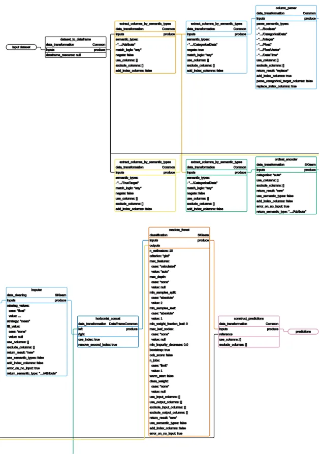
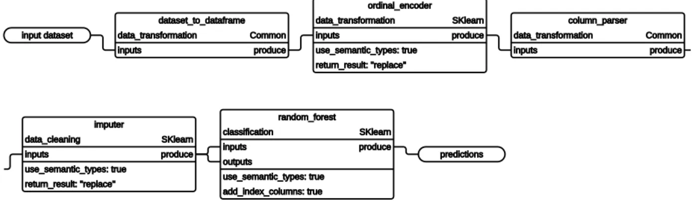
Visual representation of an example pipeline is available in Figure 3.5. The example pipeline is logically equivalent to the ML program in Figure 3.1 and is available in YAML serialization format in Appendix J.

First we convert a Dataset object to a DataFrame object. We can do this in a

straight-forward manner because the Dataset contains only one resource, a tabular DataFrame object.

After that we extract numerical and categorical attributes, and then the target column, too. When loading Dataset objects no automatic parsing of strings of any kind is done and are

values are kept as strings. Because of that we have to parse numerical attributes using an ex-plicit primitive, after which we can impute numerical attributes. We also encode categorical attributes and combine them with numerical attributes, which concludes all preprocessing of attributes. We then build a random forest model. The final step is necessary to restore the row index column which is a required part of standard predictions output of a standard

pipeline. We will discuss standard pipelines in Section 4.1. Random forest primitive does not

preserve the index column by default for compatibility with scikit-learn behavior, on which it is based.

In our example the Dataset comes with semantic information for each column and we

use it when extracting columns so that we do not have to hard-code column indices into the pipeline. If such semantic information was missing, we could have used a primitive to infer it. Using such primitive to infer semantic types is an example how populating

input dataset dataset_to_dataframe data_transformation Common produce inputs extract_columns_by_semantic_types data_transformation Common produce inputs semantic_types : -"…/Attribute" extract_columns_by_semantic_types data_transformation Common produce inputs semantic_types : -"…/CategoricalData" negate : true extract_columns_by_semantic_types data_transformation Common produce inputs semantic_types : -"…/CategoricalData" extract_columns_by_semantic_types data_transformation Common produce inputs semantic_types : -"…/T rueT arget" column_parser data_transformation Common produce inputs ordinal_encoder data_transformation SKlearn produce inputs imputer data_cleaning SKlearn produce inputs horizontal_concat data_transformation DataFrameCommon produce left right random_forest classification SKlearn produce inputs outputs construct_predictions data_transformation Common produce inputs reference predictions Figure 3.5: Visual represen tation of an example pip eline. It is a v ailable in Y AML serialization form at in App endix J.

with semantic information can be decoupled from acting on this information (in our case extracting columns).

Alternatively, we could instead extract columns by their structural type or dtype, like the ML program in Figure 3.1 does, but this is error-prone and fragile in the AutoML context because it is hard to control or predict when and how will low-level data operations in primitives change them, sometimes just as a side-effect of an operation. Semantic types are independent from data operations and do not have these shortcomings.

Observe high branching in the pipeline. We will discuss implications of branching in Section 4.2.

In this example pipeline, many primitives are transformer primitives (extending

TransformerPrimitiveBasebase class) without any parameters to learn. For some primitives we

set control hyper-parameters in the pipeline to guide their behavior, but there is no difference in their behavior between the fit phase and produce phase. Primitives for parsing, imputing, and encoding as unsupervised learner primitives (extendingUnsupervisedLearnerPrimitiveBase

base class), learning during the fit phase the properties of training data, updating their pa-rameters. After fitting in fit phase, and in whole produce phase, those parameters are then used to guide the logic of primitives when they produce outputs given input data. A su-pervised learner primitive, random forest (extending SupervisedLearnerPrimitiveBase) learns

from example attributes and targets during the fit phase and produces its own best predicted targets afterwards, during fit phase it produces predicted targets on training data and during produce phase it produces predicted targets on testing data.

The example pipeline in Figure 3.5 and Appendix J has only non-default hyper-parameter values set as part of the pipeline description. The full set of hyper-parameters defined by all primitives and their values in effect can be seen in Figure 3.6.

3.12

Problem description

Main use of a problem description in an AutoML system is to guide the system towards solving a meaningful problem given data. Our problem description is currently simple and contains:

• Task type and subtype categories with controlled vocabularies to categorize problems into a wide range of tasks, beyond just basic classification and regression.

• Which performance metrics the AutoML system should optimize for.

• Which columns in a dataset are target columns.

• A list of privileged data columns related to unavailable attributes during testing. These columns do not have data available in the test split of a dataset.

input dataset dataset_to_dataframe data_transformation Common produce inputs dataframe_resource: null extract_columns_by_semantic_types data_transformation Common produce inputs semantic_types: - "…/Attribute" match_logic: "any" negate: false use_columns: [] exclude_columns: [] add_index_columns: false extract_columns_by_semantic_types data_transformation Common produce inputs semantic_types: - "…/CategoricalData" negate: true match_logic: "any" use_columns: [] exclude_columns: [] add_index_columns: false extract_columns_by_semantic_types data_transformation Com