Intelligible Models: Recovering Low Dimensional Additive Structure For Machine Learning Models

(1)

INTELLIGIBLE MODELS: RECOVERING LOW

DIMENSIONAL ADDITIVE STRUCTURE FOR

MACHINE LEARNING MODELS

A Dissertation

Presented to the Faculty of the Graduate School of Cornell University

in Partial Fulfillment of the Requirements for the Degree of Doctor of Philosophy

by Yin Lou May 2014

(2)

c

2014 Yin Lou

(3)

INTELLIGIBLE MODELS: RECOVERING LOW DIMENSIONAL ADDITIVE STRUCTURE FOR MACHINE LEARNING MODELS

Yin Lou, Ph.D. Cornell University 2014

Different supervised learning models have different bias-variance tradeoffs. For low dimensional problems, low-bias models such boosted trees or SVMs with RBF kernels are very accurate but are unfortunately no longer interpretable by the users. For high dimensional problems, high-bias models such as regularized linear/logistic regressions are usually preferred over other models because of the curse of dimensionality and the exponentially growing hypothesis space but it is not clear whether we could further improve the accuracy from those high-bias models.

Additive modeling is an excellent tool to control the bias and variance in a finer granularity and provides a great solution to these problems. Generalized additive models (GAMs) express the hypothesis as a sum of components, where each component can include any number of variables. Therefore, by prudently selecting the components or restricting the number of complex components and carefully controlling the complexity of each selected component, GAMs are very flexible of modeling hypothesis with different biases.

This dissertation presents a family of additive models called intelligible models, which effectively recover the low dimensional additive structures. Those low dimensional additive components provide the opportunities for data scientists to investigate each simple component individually, and therefore the interpretability is significantly improved. We first present a large-scale empir-ical study of various methods for fitting GAMs. We demonstrate empirempir-ically that gradient boosting with shallow bagged trees yield the best accuracy. In

(4)

ad-dition, we propose a very efficient method of detecting pairwise feature interac-tions that scales to thousands of features. With a large-scale empirical study, we show that models with low dimensional additive components (one- and two-dimensional components) are as accurate as complex models such as random forests. Finally, we develop a method to carefully control the complexity of the intelligible models by feature selection and intelligently deciding whether the selected term is linear or nonlinear, and show that on high dimensional prob-lems we can further improve the accuracy from the popular linear models by allowing a small set of features to act nonlinearly.

(5)

BIOGRAPHICAL SKETCH

Yin Lou grew up in Shanghai, China. He had no interaction with computers until his 5th grade in elementary school. Yin started to write programs to solve puzzles during his secondary school soon after he got his first personal com-puter.

Yin graduated from the high school affiliated to Fudan University in 2005 and obtained his Bachelor of Science degree in Computer Science from Fudan University in 2009. He visited the Hong Kong University of Science and Tech-nology in Fall 2007. Yin started his doctorial program in Computer Science at Cornell University since 2009. Yin’s research interests are in the areas of data mining, statistical machine learning, information retrieval, and computer vi-sion. He has been serving as program committee member for International Conference on Machine Learning since 2012.

(6)

(7)

ACKNOWLEDGMENTS

This dissertation would not be possible without the help and influence of many people over the years. First of all I would like to thank my advisor, Johannes Gehrke, for his active support and hands-on guidance. Johannes always en-couraged me to think about big pictures and aim at solving big problems.

Rich Caruana was my external advisor and I really appreciated the influence that he had on my work. This dissertation started with the discussion with Rich and Johannes while I was interning at Microsoft Research. I was very grateful for his vision on additive modeling and for his superb support and guidance during and after the internship.

I was also very lucky to have had great collaborations with statisticians. I would like to sincerely thank Giles Hooker for providing insightful comments from the point of a statistician and for serving on my thesis committee. I would also like to thank Jacob Bien for guiding me approaching some opti-mization/theoretical problems and for his generous support and valuable ad-vice. Both of them were actively involved in my research and their expertise in statistics provided additional dimension to this work.

I would also like to thank Noah Snavely for his guidance on computer vi-sion problems. The conversation with Noah has always been inspiring and mo-tivated me for a lot of learning problems with applications on computer vision. I was very grateful to the members of my thesis committee: Johannes Gehrke, Rich Caruana, Noah Snavely, Giles Hooker and Dexter Kozen. Their constructive feedback and suggestions have helped me improve my work tremendously.

I would also like to thank Nick Craswell at Bing and Daria Sorokina at LinkedIn for their great practical advice on information retrieval and

(8)

provid-ing me the opportunity to apply this work on several industry applications. Finally, I would like to thank my parents for their endless love and support.

(9)

5.3 Our Approach . . . 72 5.3.1 Optimization . . . 72 5.3.2 Practical Issues . . . 76 5.4 Theoretical Properties . . . 78 5.4.1 Convergence . . . 78 5.4.2 An Oracle Inequality . . . 79 5.5 Scalability . . . 87 5.6 Experiments . . . 88 5.6.1 Synthetic Problem . . . 89 5.6.2 Simulation . . . 92 5.6.3 Real Problems . . . 93 5.7 Conclusion . . . 97 6 Conclusion 99 Bibliography 101

(11)

LIST OF TABLES

3.1 From Linear to Additive Models. . . 14

3.2 Preview of Empirical Results. . . 16

3.3 Datasets. . . 21

3.4 Notation for learning methods and shape functions. . . 25

3.5 RMSE for regression datasets. Each cell contains the mean RMSE ± one standard deviation. Average normalized score on five datasets (excludes synthetic) is shown in the last column, where the score is calculated as relative improvement over P-LS. . . 29

3.6 Error rate for classification datasets. Each cell contains the clas-sification error±one standard deviation. Averaged normalized score on all datasets is shown in the last column, where the score is calculated as relative improvement over P-IRLS. . . 30

4.2 RMSE for regression datasets. Each cell contains the mean RMSE ±one standard deviation. Average normalized score is shown in the last column, calculated as relative improvement over GAM. . 54

4.3 Error rate for classification datasets. Each cell contains the er-ror rate ±one standard deviation. Average normalized score is shown in the last column, calculated as relative improvement over GAM. . . 54

5.1 RMSE for synthetic dataset in Example 4. Mean RMSE ± one standard deviation is shown. . . 87

5.3 Classification error (%) for datasets in Section 5.6.3. Each cell contains the mean error±one standard deviation. . . 94

(12)

LIST OF FIGURES

3.1 Shape Functions for Synthetic Dataset in Example 1. . . 13

3.2 Shape Functions for Concrete Dataset in Example 2. . . 14

3.3 Training curves for gradient boosting and backfitting. Figure

(a), (b) and (c) show the behavior of BST-bagTR2, BST-bagTR16 and BF-bagTR on the “Concrete” regression problem, respec-tively. Figure (d), (e) and (f) illustrate behavior of BST-bagTR2, BST-bagTR16 and BF-bagTR on the “Spambase” classification,

respectively. . . 22

3.4 Shapes of features for the “Concrete” dataset produced by P-LS

(top) and BST-bagTR3 (bottom). . . 23

3.5 Shapes of features for the “Spambase” dataset produced by

P-IRLS (top) and BST-bagTR3 (bottom). . . 24

3.6 Bias-variance analysis for the six regression problems (bias = red

at bottom of bars; variance = green at top of bars). . . 32

4.1 Illustration for searching cuts on input space ofxiandxj. On the

left we show a heat map on the target for different values of xi

andxj. ciandcj are cuts forxi andxj, respectively. On the right

we show an extremely simple predictor of modeling pairwise

interaction. . . 45

4.2 Illustration for computing sum of targets for each quadrant.

Given that the value of red quadrant is known, we can easily recover values in other quadrant using marginal cumulative

his-tograms. . . 48

4.3 Illustration for computing shape function for pairwise interaction. 52

4.4 Sensitivity of FAST to the number of bins. . . 56

4.5 Precision/Cost on synthetic function. . . 57

4.6 True/Spurious heat maps. Features are discretized into 32 bins

for visualization. . . 61

4.7 Weights for pairwise interaction terms in the model. . . 61

4.8 Computational cost on real datasets. . . 62

4.9 Shapes of features and pairwise interactions for the “MSLR10k”

dataset with weights. Top two rows show top 10 strongest

fea-tures. Next two rows show top 10 strongest interactions. . . 63

5.1 Fitted f(x7) for dataset in Example 4. Black dots represent the

noisy data points. Estimated function is in red solid line and

true (linear) component is in blue dashed line. . . 66

5.2 Estimated component functions and weights for synthetic

dataset in Example 4. . . 89

5.3 Objective value vs. running time for synthetic dataset in

(13)

5.4 Results for simulation in Section 5.6.2. Each plot shows the

win-ing model for a given(δ, γ)pair. . . 92

(14)

CHAPTER 1

INTRODUCTION

1.1

Motivation

Supervised learning, in particular classification and regression, is now widely used in numerous real world applications. Examples of supervised learning based systems include fraudulent transaction detection for credit cards [21], house price prediction [56], learning to rank [43], text categorization [37], de-tecting objects in images [61], recognizing hand-written digits [12], and so on. A lot of supervised learning models for classification and regression have been de-veloped, such as linear regression [14], logistic regression [51], na¨ıve bayes [53], classification and regression trees [17], random forests [15], gradient boosted re-gression trees, support vector machines (SVMs) [23] with radial basis function kernel, etc.

Some of those models have demonstrated excellent predictive performance in low dimensional problems, while others are more suitable in high dimen-sional cases [19, 20], since those models exhibit different bias-variance tradeoff. For example, in many low dimensional problems, complex models such as en-sembles of trees, SVMs with RBF kernels are the most accurate since the amount of data is usually enough for effectively modeling the nonlinear effects in the data which cannot be captured by simple models such as linear regression or logistic regression, and therefore these low-bias models often outperform other high-bias models. On the other hand, in high dimensional cases, because of the curse of dimensionality and the exponentially growing hypothesis space, complex low-bias models often overfit and suffer from high variance, while lin-ear models with regularizations tend to offer better predictive performance by

(15)

setting up a high bias, which results in a low variance. However, there are essentially two problems.

• In many applications of low dimension, what is learned is just as

impor-tant as the accuracy of the predictions. Unfortunately, the high accuracy of complex models comes at the expense of interpretability; e.g., even the contribution of individual features to the predictions of a complex model

are difficult to understand. Is there a model which is as accurate as those

com-plex models while still provides ways for data scientists to understand the model by maintaining the intelligibility as much as possible?

• In high dimensional problems, linear models with regularizations set up a

very high bias by restricting each feature to be linear. But we are not sure whether linear model is the best model class to describe or understand the

data. Are there any other alternatives which offer better predictive performance

by more carefully balancing bias and variance?

In this thesis, we revisit the classic additive modeling and show that these two problems can be answered simultaneously by using additive models. we

present a family of additive models called intelligible models, which effectively

recover the low dimensional additive structures. Those low dimensional addi-tive components provide great opportunities for data scientists to investigate

eachsimplecomponent individually, and therefore the interpretability is largely

preserved. In addition, we present a large-scale empirical study showing that models with low dimensional additive components are as accurate as complex models such as random forests. Finally, we present a method to carefully con-trol the complexity of the intelligible models by feature selection and intelli-gently deciding whether the selected term is linear or nonlinear, and show that on high dimensional problems we can further improve the accuracy from the

(16)

popular linear models by allowing a small set of features to act nonlinearly.

1.2

Contributions and Outline

The organization and contributions of each subsequent chapter are as follows.

Chapter 2reviews classic additive modeling. We first introduce the standard generalized additive models (GAMs) that employ a one-dimensional smoother to build a restricted class of nonparametric models. Next, we review the clas-sic gradient boosting in the context of additive ensembles. Finally, we discuss the connection of additive models with simple models (such as the standard generalized linear models) and complex models (such as random forests).

Chapter 3presents our large-scale empirical study of build intelligible mod-els using GAMs. In this chapter, we consider various combinations of shape functions (a.k.a one-dimensional smoothers or base learners) and optimization algorithms [46]. Since the shape functions can be arbitrarily complex, GAMs are more accurate than simple linear models. But since they do not contain any interactions between features, they can be easily interpreted by users. Our study includes existing spline and tree-based methods for shape functions and penalized least squares, gradient boosting, and backfitting for learning GAMs. We also present a new method based on tree ensembles with an adaptive num-ber of leaves that consistently outperforms previous work. We complement our experimental results with a bias-variance analysis that explains how different shape models influence the additive model.

Chapter 4extends our previous study and proposes GA2M-models, for

Gen-eralized Additive Models plus Interactions[47]. In this chapter, we suggest adding

selected terms of interacting pairs of features to standard GAMs. Since these

(17)

GA2M-models can be visualized and interpreted by users. To explore the huge (quadratic) number of pairs of features, we develop a novel, computationally efficient method called FAST for ranking all possible pairs of features as can-didates for inclusion into the model. In a large-scale empirical study, we show the effectiveness of FAST in ranking candidate pairs of features. In addition,

we show the surprising result that GA2M have almost the same predictive

per-formance as the best full-complexity models on a number of real datasets. This postulates that for many problems, using one- and two-dimensional additive components are enough to yield models that are both intelligible and accurate.

Chapter 5studies the problem of complexity control of GAMs. In this chap-ter, we introduce generalized sparse partially linear additive models (SPLAMs), which in addition to variable selection, each variable can stay linear as in stan-dard generalized linear models (GLMs), or it can be allowed to act nonlinearly as in standard generalized additive models (GAMs) when there is sufficient ev-idence in the data. We model the problem as a convex hierarchical sparse reg-ularization problem and propose two algorithms using block coordinate gradi-ent descgradi-ent and block coordinate descgradi-ent, respectively, to solve the optimiza-tion problem. A statistical analysis of the theoretical properties for SPLAM is provided. A general technique for optimization on data-sparse problem is also

discussed. In this study, we aim to provide alternatives to `1 regularized

lin-ear models in high dimensional cases. Our large-scale experiments show that SPLAM effectively recovers the underlying additive structure and often outper-forms GLM/GAM in terms of accuracy.

(18)

CHAPTER 2

ADDITIVE MODELING

In this chapter, we review the classic additive modeling. We first intro-duce the standard generalized additive models (GAMs) that employ a one-dimensional smoother to build a restricted class of nonparametric models. Next, we review the classic boosting algorithms in the context of additive ensembles. Finally, we discuss the connection of additive models with simple models (such as the standard generalized linear models) and complex models (such as ran-dom forests).

Let D = {(xi, yi)}N1 denote a training dataset of size N, where xi =

(xi1, ..., xip) is a feature vector with p features and yi is the target (response).

We usexjto denote thejth variable in the feature space. LetLdenote some loss

function, such as squared loss, or logistic loss.

2.1

Generalized Additive Models

Generalized additive models (GAMs) are nonparametric methods which use a one-dimensional smoother to build a restricted class of nonparametric models. GAMs take the following standard form.

g(E[y]) = X

j

fj(xj) (2.1)

The function g(·) is called the link function and we call the fis shape

func-tions(a.k.a smoothers or base learners). If the link function is the identity

func-tion, Equation 2.3 describes an additive model (e.g., a regression model); if the link function is the logit function, Equation 2.3 describes a generalized addi-tive model (e.g., a classification model). These two link functions are the most common ones used in most real applications.

(19)

Algorithm 1Backfitting for Regression 1: fj ←0 2: form= 1toM do 3: forj = 1topdo 4: R ← {xij, yi− P k6=jfk}N1

5: Learn shaping functionS :xj →yusingRas training dataset

6: fj ←S

Classic approach to learning additive models is the backfitting algo-rithm [32]. The algoalgo-rithm starts with an initial guess of all shape functions (such

as setting them all to zero). The first functionf1is then learned using the

train-ing set with the goal to predict y. Then we learn the second shape functionf2

on the residualsy−f1(x1), i.e., using training set{(xi2, yi−f1(xi1))}N1 . The third

shape function is trained on the residualsy−f1(x1)−f2(x2), and so on. After

we have trained all pshape functions, the first shape function is discarded and

retrained on the residuals of the otherp−1shape functions. Note that

backfit-ting is a functional form of the “Gauss-Seidel” algorithm and its convergence is usually guaranteed [32]. Algorithm 1 summarizes the backfitting algorithm.

For classification problems, the classic approach is to use a generalized ver-sion of the backfitting algorithm called the “Local Scoring Algorithm” [32], as

summarized in Algorithm 2 . LetF(x) = P

jfj(xj), we form the working

re-sponse (Line 3) ˜ yi =F(xi) + 1(yi = 1)−p(xi) p(xi)(1−p(xi)) ,

where p(xi) = 1+exp(−1F(xi)). We then apply the weighted backfitting algorithm

(20)

Algorithm 2Backfitting for Classification 1: fj ←0 2: form= 1toM do 3: y˜i =F(xi) + 1(yi =1)−p(xi) p(xi)(1−p(xi)), fori= 1, ..., N 4: wi ←p(xi)(1−p(xi))

5: Apply weighted backfitting algorithm in Algorithm 1

2.2

Additive Ensembles

In this section, we describe gradient boosted tree ensembles [25, 26]. Gradient boosted trees are additive ensembles which greedily build small steps (trees) to fit the data. The final prediction is the sum of all functions in the ensemble. Since gradient boosting often uses regression trees as base learners, it is also called gradient boosted regression trees (GBRT). GBRT has been widely used in a lot of industry-scale real applications.

Gradient boosting framework [26] is described in Algorithm 3. Given the

loss function L, gradient boosting adopts a “greedy stagewise” approach to

build an additive functionFM,

FM(x) = M

X

m=1

ρmh(x;am),

such that, at each stagem,

{ρm,am}= arg min ρ,a N X i=1 L(yi, Fm−1+ρh(xi;a))

Here h(x;a) is a “weak” learner. Instead of directly solving this difficult

problem, [26] approximately conducted steepest descent in function space by solving a least square problem (Line 4),

am = arg min a,ρ N X i=1 [−gm(xi)−ρh(xi;a)]2, where −gm(xi) = − ∂L(yi, F(xi))

(21)

Algorithm 3Gradient Boosting 1: F0(x)←arg minρ PN i=1L(yi, ρ) 2: form= 1toM do 3: y˜i ← − h ∂L(yi,F(xi)) ∂F(xi) i F(x)=Fm−1(x) , i= 1, ..., N 4: am ←arg mina,ρPN_i₌₁[˜yi −ρh(xi;a)]2 5: ρm ←arg minρ PN i=1L(yi, Fm−1(xi) +ρh(xi;am)) 6: Fm(x)←Fm−1(x) +ρmh(x;am)

Algorithm 4GBRT for Regression

1: F0(x)←y¯

2: form= 1toM do

3: y˜i ←yi−Fm−1(xi), i= 1, ..., N

4: {Rjm}J1 ←aJ-terminal node tree trained on{(xi,y˜i)}N1

5: Fm(x)←Fm−1(x) +PJ_j₌₁γjm1(x∈Rjm)

is the steepest descent direction in the N-dimensional data space at Fm−1(x).

For the other coefficientρm, a line search is performed (Line 5),

ρm ←arg min ρ N X i=1 L(yi, Fm−1(xi) +ρh(xi;am)).

Algorithm 4 describes the GBRT algorithm for regression problems. At each iteration, gradient boosting forms the current residual (Line 3) and builds a

J-terminal node regression tree with γj denoting the prediction value for leaf

Rj(Line 4), which is then added to the ensemble (Line 5).

Algorithm 5 describes the GBRT algorithm for binary classification prob-lems. Here the loss function is the negative binomial log-likelihood,

L(y, F) = log(1 + exp(−2yF)), y ∈ {−1,1}

The pseudo response is (Line 3),

˜ yi =− ∂L(yi, F(xi)) ∂F(xi) F(x)=Fm−1(x) = 2yi 1 + exp(2yiF(xi)) The line search becomes

ρm = arg min N

X

i=1

(22)

Algorithm 5GBRT for Classification

1: F(xi)←0

2: form= 1toM do

3: y˜i ← _1+exp(22y_yi_i_F₍_x_i₎₎, i= 1, ..., N

4: {Rjm}J1 ←aJ-terminal node tree trained on{(xi,y˜i)}N1

5: γjm = P xij∈_Rjm˜yi P xij∈_Rjm|˜yi|(2−|y˜i|), j = 1, ..., J 6: F(xi)←F(xi) +PJ_j₌₁γjm1(xi ∈Rjm)

With J-terminal node regression tree as base learners (Line 4), we use the

strategy of separate updates in each terminal nodeRjm,

γjm = arg min γ

X

xi∈Rjm

log(1 + exp(−2yi(Fm−1(xi) +γ))). (2.2) There is no closed form solution to 2.2, we approximate it by a single Newton-Raphon step (Line 5),

γjm= X xi∈Rjm ˜ yi/ X xi∈Rjm |y˜i|(2− |y˜i|) Finally the updated tree is added to the ensemble (Line 6).

The gradient boosting algorithm is deterministic, stochastic gradient boost-ing further improves the predictive performance by addboost-ing randomness at each boosting iteration [27]. In particular, at each boosting iteration, a bootstrap sam-ple is drawn and the standard gradient boosting step is applied on the samsam-pled data instead of the full data.

Another popular boosted tree algorithm for classification problems is Logit-Boost [25]. LogitLogit-Boost differs from GBRT in that LogitLogit-Boost forms the pseudo residual by taking the point-wise Newton gradient. As shown in Algorithm 6, the Newton-Raphson step is pushed before the construction of the tree (Line 3),

wherey_i∗ = 1ifyi = 1and yi∗ = 0when yi = −1. A weight is assigned to each

(23)

Algorithm 6LogitBoost for Classification

1: Start with weightswi = 1/N,i= 1, ..., N,F(x) = 0and probability estimates

p(xi) = 1/2. 2: form= 1toM do 3: zi ← y∗ i−p(xi) p(xi)(1−p(xi)), i= 1, ..., N 4: wi ←p(xi)(1−p(xi))

5: fm(x)←aJ-leaf tree trained on{(xi, zi)}N1 using weights{wi}N1

6: F(xi)←F(xi) + 1₂fm(x)

7: p(x)← _exp(_F₍exp(_x_))+exp(−F(x))_F₍_x₎₎

the leaf values. Liet al. showed that LogitBoost exhibits better empirical

con-vergence than GBRT [42], while Friedman pointed out the weighting scheme in LogitBoost can sometimes cause numerical instability [26].

2.3

Discussion

A special class of GAMs is called generalized linear molds (GLMs), which have the following form.

g(E[y]) =β0+

X

j

βjxj (2.3)

It is clear that standard GAMs subsume the class of GLMs by forcing each component to be linear. Therefore, GAMs have lower bias than GLMs.

On the other hand, when each component of GAMs can use all features, the model class is equivalent to the following.

y=f(x1, ..., xp) (2.4)

This is a special form of additive models in which only one component is in the model. Complex methods such as classification and regression trees, ran-dom forests, etc., directly build models of this form.

(24)

compo-nents as follows. g(E[y]) =X j fj(xj) + X ij fij(xi, xj) + X ijk f(xi, xj, xk) +... (2.5)

Components involving more than one features are called statistical interac-tions. By adding higher order interactions, we gradually move from standard GAMs to full complexity models such as random forests. As we will see later in Chapter 4, adding pairwise interactions is usually enough to build accurate models while maintaining the intelligibility as much as possible.

(25)

CHAPTER 3

INTELLIGIBLE MODELS FOR CLASSIFICATION AND REGRESSION

Everything should be made as simple as possible, but not simpler.

— Albert Einstein.

3.1

Introduction

Classification and regression are two of the most important data min-ing/machine learning tasks. Currently, the most accurate methods on many datasets are complex models such as boosted trees, SVMs, or deep neural nets.

However, in many applications what is learned is just as important as the

ac-curacy of the predictions. Unfortunately, the high acac-curacy of complex models comes at the expense of interpretability; e.g., even the contribution of individual features to the predictions of a complex model are difficult to understand.

The goal of this work is to construct accurate models that are interpretable. By interpretability we mean that users can understand the contribution of indi-vidual features in the model; e.g., we want models that can quantify the impact of each predictor. This desiderata permits arbitrary complex relationships be-tween individual features and the target, but excludes models with complex interactions between features. Thus in this chapter we fit models of the form:

g(E[y]) =f1(x1) +...+fn(xn), (3.1)

which are known asgeneralized additive modelsin the literature [32, 68]. The

func-tiong(·)is called the link functionand we call thefisshape functions. If the link

function is the identity, Equation 3.1 describes an additive model (e.g., a regres-sion model); if the link function is the logit function, Equation 3.1 describes a generalized additive model (e.g., a classification model).

(26)

0 1 2 3 4 −2 −1 0 1 2 0.0 0.5 1.0 1.5 2.0 −2 −1 0 1 2 0 5 10 15 −2 −1 0 1 2 f1(x1) f2(x2) f3(x3) 0 10 20 30 40 50 −2 −1 0 1 2 0.0 0.2 0.4 0.6 0.8 1.0 1.2 1.4 −2 −1 0 1 2 0 1 2 3 4 5 6 −2 −1 0 1 2 f4(x4) f5(x5) f6(x6)

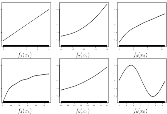
Figure 3.1: Shape Functions for Synthetic Dataset in Example 1.

Example 1. Assume we are given a dataset with 10,000 points generated from the

modely=x1+x22+

√

x3+ log(x4) + exp(x5) + 2 sin(x6) +, where∼ N(0,1). After

fitting an additive model to the data of the form shown in Equation 3.1, we can visualize

the contribution ofxis as shown in Figure 3.1: Because predictions are a linear function

of thefi(xi), scatterplots offi(xi)on the y-axis vs. xion the x-axis allow us to visualize

the shape function that relates thefi(xi)to the xi, thus we can easily understand the

contribution ofxi to the prediction.

Because the data in Example 1 was drawn from a model with no interactions between features, a model of the form in Equation 3.1 is able to fit the data perfectly (modulo noise). However, data are not always so simple in practice. As a second example, consider a real dataset where there may be interactions between features.

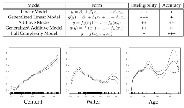
Example 2. The “Concrete” dataset relates the compressive strength of concrete to its age and ingredients. The dataset contains 1030 points with eight numerical features.

(27)

Table 3.1: From Linear to Additive Models.

Model Form Intelligibility Accuracy Linear Model y=β0+β1x1+...+βnxn +++ + Generalized Linear Model g(y) =β0+β1x1+...+βnxn +++ + Additive Model y=f1(x1) +...+fn(xn) ++ ++ Generalized Additive Model g(y) =f1(x1) +...+fn(xn) ++ ++ Full Complexity Model y=f(x1, ..., xn) + +++

100 200 300 400 500 −20 −10 0 10 20 30 40 120 140 160 180 200 220 240 −20 −10 0 10 20 30 40 0 100 200 300 −20 −10 0 10 20 30 40

Cement Water Age

Figure 3.2: Shape Functions for Concrete Dataset in Example 2.

We again fit an additive model of the form in Equation 3.1. Figure 3.2 shows scatter plots of the shape functions learned for three of the eight features. As we can see from the figure, the compressibility of concrete depends nearly linearly on the Cement feature, but it is a complex non-linear function of the Water and Age features; we say that the model

hasshaped these features. A linear model without the ability to shape features would

have worse fit because it cannot capture these non-linearities. Moreover, an attempt to interpret the contribution of features by examining the slopes of a simple linear model would be misleading; the additive model yields much better fit to the data while still

remaining intelligible.1

As we saw in the examples, additive models explicitly decompose a complex function into one-dimensional components, its shape functions. Note, however,

that the shape functions themselves may be non-linear: Each featurexican have

(28)

a complex non-linear shapefi(xi), and thus the accuracy of additive models can be significantly higher than the accuracy of simple linear models. Table 3.1 sum-marizes the differences between models of different complexity that we con-sider in this chapter. Linear models, and generalized linear models (GLMs) are the most intelligible, but often the least accurate. Additive models, and general-ized additive models (GAMs) are more accurate than GLMs on many data sets because they capture non-linear relationships between (individual) features and the response, but retain much of the intelligibility of linear models. Full com-plexity models such as ensembles of trees are more accurate on many datasets because they model both non-linearity and interaction, but are so complex that it is nearly impossible to interpret them.

In this chapter we present the results of (to the best of our knowledge) the largest experimental study of GAMs. We consider shape functions based on splines [68] and boosted stumps [26], as well as novel shape functions based on bagged and boosted ensembles of trees that choose the number of leaves adaptively. We experiment with (iteratively re-weighted) least squares, gradi-ent boosting, and backfitting to both iteratively refine the shape functions and construct the linear model of the shaped features. We apply these methods to six classification and six regression tasks. For comparison, we fit simple linear models as a baseline. We also fit unrestricted ensembles of trees as full complex-ity models to get an idea of what accuracy is achievable.

Table 3.2 summarizes the key findings of our study. Entries in the table are the average accuracies on the regression and classification datasets, normal-ized by the accuracy of Penalnormal-ized (Iteratively Re-weighted) Least Squares with Splines (P-LS/P-IRLS). As expected, the accuracy of GAMs falls between that of linear/logistic regression without feature shaping and full-complexity models

(29)

Table 3.2: Preview of Empirical Results.

Model Regression Classification Mean

Linear/Logistic 1.68 1.22 1.45 P-LS/P-IRLS 1.00 1.00 1.00 BST-SP 1.03 1.00 1.02 BF-SP 1.00 1.00 1.00 BST-bagTR2 0.96 0.96 0.96 BST-bagTR3 0.97 0.94 0.96 BST-bagTR4 0.99 0.95 0.97 BST-bagTRX 0.95 0.94 0.95 Random Forest 0.88 0.80 0.84

such as random forests. However, surprisingly, the best GAM models have ac-curacy much closer to the full-complexity models than to the linear models. Our results show that bagged trees with 2-4 leaves as shape functions in combina-tion with gradient boosting as learning method (Methods bag-TR2 to BST-bag-TR4) outperform all other methods on most datasets. Our novel method of adaptively selecting the right number of leaves (Method BST-bagTRX) is almost always even better, and thus we recommend it as the method of choice. On average, this method reduces loss by about 5% over previous GAM models, a significant improvement in practice.

The rest of the chapter is structured as follows. Section 3.2 presents algo-rithms for fitting generalized additive models with various shape functions and learning methods. Section 3.3 describes our experimental setup, Section 3.4 presents the results and their interpretation, followed by a discussion in Section 3.5 and an overview of related work in Section 3.6. We conclude in Section 3.7.

3.2

Methodology

LetD = {(xi, yi)}1N denote a training dataset of sizeN, wherexi = (xi1, ..., xin)

(30)

con-sider both regression problems whereyi ∈Rand binary classification problems

where yi ∈ {1,−1}. Given a model F, let F(xi) denote the prediction of the

model for data point xi. Our goal in both classification and regression is to

minimize the expected value of some loss functionL(y, F(x)).

We are working with generalized additive models of the form in Equa-tion 3.1. To train such models we have to select (i) the shape funcEqua-tions for indi-vidual features and (ii) the learning method used to train the overall model. We discuss these two choices next.

3.2.1

Shape Functions

In our study we consider two classes of shape functions: regression splines and trees or ensembles of trees. Note that all shape functions relate a single attribute to the target.

Regression Splines. We consider regression splines of degreedof the form

y=

d

P

k=1

βkbk(x).

Trees and Ensembles of Trees.We also use binary trees and ensembles of bi-nary trees with largest variance reduction as split selection method. We control tree complexity by either fixing the number of leaves or by disallowing leaves

that have fewer than anα-fraction of the number of training examples.

We consider the following ensemble variants:

• Single Tree. We use a single regression tree as a shape function.

• Bagged Trees. We use the well-known technique of bagging to reducing

variance [10].

• Boosted Trees. We use gradient boosting, where each successive tree tries

(31)

• Boosted Bagged Trees. We use a bagged ensemble in each step of gradient boosting [26], resulting in a boosted ensemble of bagged trees.

3.2.2

Generalized Additive Models

We consider three different methods for fitting additive models in our study: Least squares fitting for learning regression spline shape functions, and gradi-ent boosting and backfitting for learning tree and tree ensemble shape functions. We review them here briefly for completeness although we would like to em-phasize that these methods are not a contribution of this thesis.

Least Squares

Fitting a spline reduces to learning the weights βk(x) for the basis functions

bk(x). Learning the weights can be reduced to fitting a linear model y = Xβ,

whereXi = [b1(xi1), ..., bk(xin)]; the coefficients of the linear model can be com-puted exactly using the least squares method [68]. To control smoothness, there

is a “wiggliness” penalty: we minimizeky−Xβk+λP

i

R

[f_i00(xi)]2dxwith the

smoothing parameter λ. Large values of λ lead to a straight line for fi while

low values of λallow the spline to fit closely to the data. We use thin plate

re-gression splines from the R package “mgcv” [68] that automatically selects the best values for the parameters of the splines [67]. We call this method penalized least-squares (P-LS) in our experiments.

The fitting of an additive logistic regression model using splines is similarly reduced to fitting a logistic regression with a different basis, which can be solved using penalized-iteratively reweighted least squares (P-IRLS) [68].

(32)

Gradient Boosting

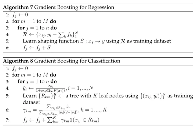
We use standard gradient boosting [26, 27] with one difference: Since we want to learn shape functions for all features, in each iteration of boosting we cycle sequentially through all features. For completeness, we include pseudo-code in Algorithms 7 and 8. In Algorithm 7, we first set all shape functions to zero

(Line 1). Then we loop overM iterations (Line 2) and over all features (Line 3)

and then calculate the residuals (Line 4). We then learn then one-dimensional function to predict the residuals (Line 5) and add it to the shape function (Line 6).

Backfitting

A popular algorithm for learning additive models is the backfitting algo-rithm [32]. The algoalgo-rithm starts with an initial guess of all shape functions (such

as setting them all to zero). The first shape functionf1is then learned using the

training set with the goal to predict y. Then we learn the second shape

func-tion f2 on the residuals y−f1(x1), i.e., using training set {(xi2, yi −f1(xi1))}N1 .

The third shape function is trained on the residuals y −f1(x1) −f2(x2), and

so on. After we have trainedn shape functions, the first shape function is

dis-carded and retrained on the residuals of the othern −1 shape functions. Note

that backfitting is a form of the “Gauss-Seidel” algorithm and its convergence is usually guaranteed [32]. Its pseudocode looks identical to Algorithm 7 except

that pseudo residual is formed by excluding currentfj in Line 4 and Line 6 is

replaced byfj ←S.

To fit an additive logistic regression model, we can use a generalized version of the backfitting algorithm called the “Local Scoring Algorithm” [32], which is

(33)

Algorithm 7Gradient Boosting for Regression 1: fj ←0 2: form= 1toM do 3: forj = 1tondo 4: R ← {xij, yi− P kfk}N1

5: Learn shaping functionS :xj →yusingRas training dataset

6: fj ←fj +S

Algorithm 8Gradient Boosting for Classification

1: fj ←0

2: form= 1toM do 3: forj = 1tondo

4: y˜i ← _1+exp(22y_yi_i_F₍_x_i₎₎, i= 1, ..., N

5: Learn{Rkm}K1 ←a tree withK leaf nodes using{(xij,y˜i)}N1 as training

dataset 6: γkm= P xij∈_Rkmy˜i P xij∈_Rkm|˜yi|(2−|˜yi|), k= 1, ..., K 7: fj ←fj + PK k=1γkm1(xij ∈Rkm)

a general method for fitting generalized additive models. We form the response

˜

yi =F(xi) +

1(yi = 1)−p(xi)

p(xi)(1−p(xi))

,

where p(xi) = _1+exp(−1_F₍_x_i₎₎. We then apply the weighted backfitting algorithm

to the responsey˜i with observation weightsp(xi)(1−p(xi))[32].

3.3

Experimental Setup

In this section we describe the experimental design.

3.3.1

Datasets

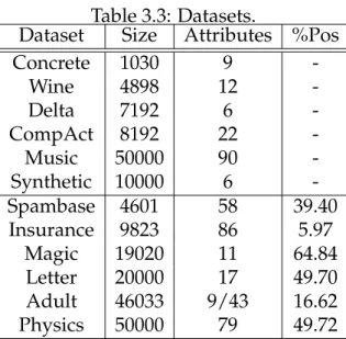
We selected datasets of low-to-medium dimensionality with at least 1000 points. Table 3.3 summarizes the characteristics of the 12 datasets. One of the regression datasets is a synthetic problem used to illustrate feature shaping (but we do not use the results on this dataset when comparing the accuracy of the methods).

(34)

Table 3.3: Datasets.

Dataset Size Attributes %Pos

Concrete 1030 9 -Wine 4898 12 -Delta 7192 6 -CompAct 8192 22 -Music 50000 90 -Synthetic 10000 6 -Spambase 4601 58 39.40 Insurance 9823 86 5.97 Magic 19020 11 64.84 Letter 20000 17 49.70 Adult 46033 9/43 16.62 Physics 50000 79 49.72

The “Concrete,” “Wine,” and “Music” regression datasets are from the UCI repository [1]; “Delta” is the task of controlling the ailerons of a F16 aircraft [2]; “CompAct” is a regression dataset from the Delve repository that describes the state of multiuser computers [3]. The synthetic dataset was described in Exam-ple 1.

The “Spambase,” “Insurance,” “Magic,” “Letter” and “Adult” classification datasets are from the UCI repository. “Adult” contains nominal attributes that we transformed to boolean attributes (one boolean per value). “Letter” has been converted to a binary problem by using A-M as positives and the rest as nega-tives. The “Physics” dataset is from the KDD Cup 2004 [4].

3.3.2

Methods

Recall from Section 3.2 that we have two different types of shape functions and three different methods of learning generalized additive models; see Ta-ble 3.4 for an overview of these methods and their names. While penalized least squares for regression (P-LS) and penalized iteratively re-weighted least squares

(35)

2 4 6 8 10 12 14 16 0 200 400 600 800 training validation test 2 4 6 8 10 12 14 16 0 200 400 600 800 training validation test 2 4 6 8 10 12 14 0 200 400 600 800 training validation test

(a) BST-bagTR2 (b) BST-bagTR16 (c) BF-bagTR

0 0.05 0.1 0.15 0.2 0.25 0.3 0.35 0 1000 2000 2900 training validation test 0 0.05 0.1 0.15 0.2 0.25 0.3 0.35 0 1000 2000 2900 training validation test 0 0.05 0.1 0.15 0.2 0.25 0.3 0.35 0 10000 20000 training validation test

(d) BST-bagTR2 (e) BST-bagTR16 (f) BF-bagTR

Figure 3.3: Training curves for gradient boosting and backfitting. Figure (a), (b) and (c) show the behavior of BST-bagTR2, BST-bagTR16 and BF-bagTR on the “Concrete” regression problem, respectively. Figure (d), (e) and (f) illustrate behavior of BST-bagTR2, BST-bagTR16 and BF-bagTR on the “Spambase” clas-sification, respectively.

for classification (P-IRLS) only work with splines, gradient boosting and back-fitting can be applied to both splines and ensembles of trees.

In gradient boosting, we vary the number of leaves in the bagged or boosted

trees: 2,3,4,8,12 to 16 (indicated by appending this number to the method

names). Trained models will containM such trees for each shape function

af-terM iterations. In backfitting, we re-build the shape function for each feature

from scratch in each round, so the shape function needs to have enough expres-sive power to capture a complex function. Thus we control the complexity of

the tree not by the number of leaves, but by adaptively choosing a parameterα

that stops splitting nodes smaller than anα fraction of the size of the training

data; we varyα ∈ {0.00125,0.025,0.05,0.1,0.15,0.2,0.25,0.3,0.35,0.4,0.45,0.5}. A summary of the combinations of shape functions and learning methods can be found in Table 3.4.

(36)

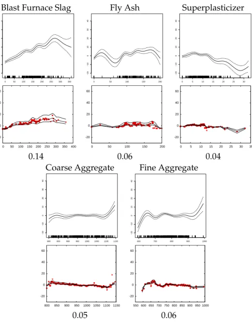
Blast Furnace Slag Fly Ash Superplasticizer 0 50 100 150 200 250 300 350 −20 −10 0 10 20 30 40 0 50 100 150 200 −20 −10 0 10 20 30 40 0 5 10 15 20 25 30 −20 −10 0 10 20 30 40 -20 0 20 40 60 0 50 100 150 200 250 300 350 400 -20 0 20 40 60 0 50 100 150 200 -20 0 20 40 60 0 5 10 15 20 25 30 35 0.14 0.06 0.04

Coarse Aggregate Fine Aggregate

800 850 900 950 1000 1050 1100 1150 −20 −10 0 10 20 30 40 600 700 800 900 1000 −20 −10 0 10 20 30 40 -20 0 20 40 60 800 850 900 950 1000 1050 1100 1150 -20 0 20 40 60 550 600 650 700 750 800 850 900 950 1000 0.05 0.06

Figure 3.4: Shapes of features for the “Concrete” dataset produced by P-LS (top) and BST-bagTR3 (bottom).

Beyond the parameters that we already discussed, P-LS and P-IRLS have a

parameterλ, which is estimated using generalized cross validation as discussed

in Section 3.2. We do not fix the number of iterations for gradient boosting and backfitting but instead run these methods until convergence as follows: We divide the training set into five partitions. We then set aside one of the partitions

(37)

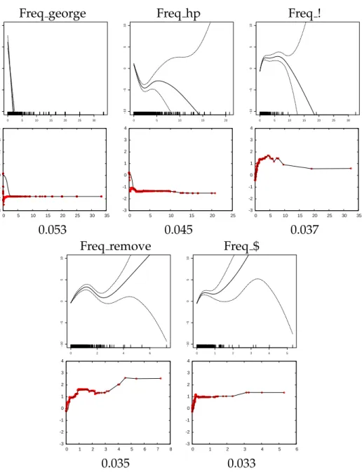
Freq george Freq hp Freq ! 0 5 10 15 20 25 30 −10 −5 0 5 10 0 5 10 15 20 −10 −5 0 5 10 0 5 10 15 20 25 30 −10 −5 0 5 10 -3 -2 -1 0 1 2 3 4 0 5 10 15 20 25 30 35 -3 -2 -1 0 1 2 3 4 0 5 10 15 20 25 -3 -2 -1 0 1 2 3 4 0 5 10 15 20 25 30 35 0.053 0.045 0.037

Freq remove Freq $

0 2 4 6 −10 −5 0 5 10 0 1 2 3 4 5 −10 −5 0 5 10 -3 -2 -1 0 1 2 3 4 0 1 2 3 4 5 6 7 8 -3 -2 -1 0 1 2 3 4 0 1 2 3 4 5 6 0.035 0.033

Figure 3.5: Shapes of features for the “Spambase” dataset produced by P-IRLS (top) and BST-bagTR3 (bottom).

as a validation set, train the model on the remaining four partitions, and use the validation set to check for convergence. We repeat this process five times and

then computeM, the average number of iterations until convergence across the

five iterations. We then re-train the model using the whole training set forM

(38)

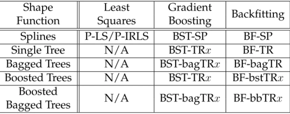
Table 3.4: Notation for learning methods and shape functions.

Shape Least Gradient

Backfitting

Function Squares Boosting

Splines P-LS/P-IRLS BST-SP BF-SP

Single Tree N/A BST-TRx BF-TR

Bagged Trees N/A BST-bagTRx BF-bagTR

Boosted Trees N/A BST-TRx BF-bstTRx

Boosted

N/A BST-bagTRx BF-bbTRx

Bagged Trees

αfor each partition and average them to train the final model using the whole

training dataset.

3.3.3

Metrics

For regression problems, we report the root mean squared error (RMSE) for lin-ear regression (no feature shaping), additive models with shaping with splines or trees (penalized least squares, gradient boosting and backfitting), and un-restricted full-complexity models (random forest regression trees and Additive Groves [5, 59]).

For classification problems, we report the error rates for logistic regres-sion, generalized additive models with splines or trees (penalized iteratively re-weighted least squares, gradient boosting and backfitting), and full-complexity

unrestricted models (random forests [15]).2

In all experiments we use 100 trees for bagging. We do not notice significant improvements by using more iterations of bagging. For Additive Groves, the number of trees is automatically selected by the algorithm on the validation set. For P-LS and P-IRLS, we use an R package called “mgcv” [68]. We perform

(39)

5-fold cross validation for all experiments.3

3.4

Results

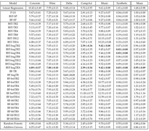
The regression and classification results are presented in Table 3.5 and Table 3.6, respectively. We report means and standard deviations on the 5-fold cross val-idation test-sets. To facilitate comparison across multiple datasets, we com-pute normalized scores that average the performance of each method across the datasets, normalized by the accuracy of P-LS/P-IRLS on each dataset.

Table 3.5 and Table 3.6 are laid out as follows: The top of each table shows results for linear/logistic regression (no feature shaping) and the traditional spline-based GAM models P-LS/P-IRLS, BST-SP, and BF-SP. The middle of the tables present results for new methods that do feature shaping with trees in-stead of splines such as boosted size-limited trees (e.g., BST-TR3), boosted-bagged size-limited trees (e.g., BST-bagTR3), backfitting of boosted trees (e.g., BF-bstTR3), and backfitting of boosted-bagged trees (e.g., BF-bbTR3). The bot-tom of each table presents results for unrestricted full-complexity models such as random forests and additive groves. Our goal is to devise more powerful GAM models that are as close in accuracy as possible to the full-complexity models, while preserving the intelligibility of linear models.

Several clear patterns emerge in both tables.

(1) There is a large gap in accuracy between linear methods that do not do feature shaping (linear or logistic regression) and most methods that perform feature shaping. For example, on average the spline-based P-LS GAM model has 60% lower normalized RMSE than vanilla linear regression. Similarly, on 3_{We use 5-fold instead of 10-fold cross validation because some of the experiments are very}

(40)

average, P-IRLS is about 20% more accurate than logistic regression.

(2) The new tree-based shaping methods are more accurate than the spline-based methods as long as model complexity (and variance — see Section 3.5.1) is controlled. In both tables, the most accurate tree-based GAM models use boosted-bagged trees that are size-limited to 2-4 leaves.

(3) Unrestricted full-complexity models such as random forests and additive groves are more accurate than any of the GAM models because they are able to model feature interactions, which linear models of shaped features cannot capture. Our goal is to push the accuracy of linear shaped models as close as possible to the accuracy of these unrestricted full-complexity models.

Looking more closely at the results for models that shape features with trees, the most accurate model on average is bagTR2 for regression, and BST-bagTR3 for classification. Models that use more leaves are consistently less accurate than comparable models with 2-4 leaves. It is critical to control tree complexity when boosting trees for feature shaping. Moreover, the most ac-curate methods used bagging inside of boosting to reduce variance. (More on model variance in Section 3.5.1.) Finally, on the regression problems, methods based on gradient boosting of residuals slightly edged out the methods based on backfitting, though the difference is not statistically significant. On the classifi-cation problems, however, where backfitting is performed on pseudo-residuals, there were stability problems that caused some runs to diverge or fail to termi-nate. Overall, tree-based shaping methods based on gradient-boosting appear to be preferable to tree-based methods based on backfitting because the gradient boosting methods may be a little more accurate, are often faster, and on some problems are more robust.

(41)

ac-curacy for GAMs, on most problems they are not able to close the gap with unrestricted full-complexity models such as random forests. For example, all linear methods have much worse RMSE on the wine regression problem than the unrestricted random forest model. On problems where feature interaction is important, linear models without interaction terms must be less accurate.

3.4.1

Model Selection

There is a risk when comparing many parameterizations of a new method against a small number of baseline methods, that the new method will appear to be better because selecting the best model on the test set leads to overfitting to the test sets. To avoid this, the table includes results for a method called

“BST-bagTRX” that uses the cross-validation validation sets (notthe CV test sets) to

pick the best parameters from the BST-bagTRx models for each dataset. This

method is not biased by looking at results on test sets, is fully automatic and thus does not depend on human judgement, and is able to select different pa-rameters for each problem. The results in Table 3.5 and Table 3.6 suggest that BST-bagTRX is more accurate than any single fixed parameterization. Looking at the models selected by BST-bagTRX, we see that BST-bagTRX usually picks models with 2, 3 or 4 leaves, and that the model it selects often is the one with the best test-set performance. On both the regression and classification datasets, BF-bagTRX is significantly more accurate than any of the models that use splines for feature shaping.

(42)

Table 3.5: RMSE for regression datasets. Each cell contains the mean RMSE±

one standard deviation. Average normalized score on five datasets (excludes synthetic) is shown in the last column, where the score is calculated as relative improvement over P-LS.

Model Concrete Wine Delta CompAct Music Synthetic Mean Linear Regression 10.43±0.49 7.55±0.13 5.68±0.14 9.72±0.55 9.61±0.09 1.01±0.00 1.68±0.98 P-LS 5.67±0.41 7.25±0.21 5.67±0.16 2.81±0.13 9.27±0.07 0.04±0.00 1.00±0.00 BST-SP 5.79±0.37 7.27±0.18 5.68±0.18 3.19±0.37 9.29±0.08 0.04±0.00 1.03±0.06 BF-SP 5.66±0.42 7.25±0.21 5.67±0.17 2.77±0.06 9.27±0.08 0.04±0.00 1.00±0.01 BST-TR2 5.19±0.39 7.17±0.10 5.75±0.18 2.68±0.33 9.55±0.08 0.11±0.00 0.98±0.08 BST-TR3 5.13±0.37 7.20±0.16 5.82±0.19 3.18±0.45 9.77±0.07 0.05±0.01 1.02±0.11 BST-TR4 5.24±0.39 7.24±0.15 5.83±0.21 3.70±0.52 9.88±0.09 0.07±0.01 1.07±0.15 BST-TR8 5.57±0.61 7.35±0.17 5.97±0.22 5.07±0.54 10.03±0.10 0.19±0.02 1.19±0.33 BST-TR12 5.92±0.63 7.39±0.13 6.03±0.19 6.59±0.71 10.15±0.07 0.26±0.02 1.31±0.54 BST-TR16 6.08±0.37 7.41±0.23 6.09±0.19 7.07±1.01 10.23±0.08 0.33±0.03 1.36±0.60 BST-bagTR2 5.06±0.39 7.05±0.11 5.67±0.20 2.59±0.34 9.42±0.08 0.07±0.00 0.96±0.08 BST-bagTR3 4.93±0.41 7.01±0.10 5.67±0.20 2.82±0.35 9.45±0.07 0.03±0.00 0.97±0.09 BST-bagTR4 4.99±0.43 7.01±0.12 5.70±0.20 2.95±0.35 9.46±0.08 0.03±0.00 0.99±0.09 BST-bagTR8 5.04±0.43 7.04±0.13 5.79±0.18 3.40±0.34 9.48±0.08 0.06±0.00 1.02±0.13 BST-bagTR12 5.11±0.44 7.07±0.15 5.85±0.18 3.76±0.33 9.50±0.07 0.07±0.00 1.05±0.16 BST-bagTR16 5.18±0.49 7.10±0.18 5.91±0.20 4.16±0.39 9.52±0.09 0.09±0.00 1.09±0.21 BST-bagTRX 4.89±0.37 7.00±0.10 5.65±0.20 2.59±0.34 9.42±0.08 0.03±0.00 0.95±0.09 BF-TR 5.80±0.60 7.19±0.09 5.67±0.21 2.81±0.25 9.88±0.08 0.06±0.03 1.02±0.07 BF-bagTR 5.10±0.49 7.02±0.13 5.61±0.21 2.69±0.31 9.43±0.07 0.04±0.00 0.97±0.07 BF-bstTR2 5.11±0.37 7.14±0.11 5.73±0.20 2.66±0.35 9.62±0.07 0.13±0.01 0.98±0.08 BF-bstTR3 5.21±0.38 7.29±0.19 5.84±0.21 4.38±0.24 10.77±0.10 0.04±0.01 1.14±0.24 BF-bstTR4 5.49±0.72 7.44±0.20 5.94±0.21 4.97±0.73 11.24±0.07 0.06±0.03 1.21±0.33 BF-bstTR8 6.74±0.76 7.93±0.32 6.08±0.24 9.18±0.77 12.08±0.07 0.04±0.01 1.59±0.87 BF-bstTR12 7.13±0.68 8.10±0.27 6.15±0.24 11.20±0.72 12.31±0.15 0.08±0.03 1.76±1.16 BF-bstTR16 7.22±0.73 8.33±0.35 6.18±0.24 11.41±0.29 12.59±0.10 0.11±0.08 1.79±1.17 BF-bbTR2 5.13±0.41 7.05±0.12 5.66±0.19 2.59±0.37 9.50±0.07 0.12±0.00 0.97±0.08 BF-bbTR3 5.15±0.44 7.07±0.17 5.74±0.20 2.85±0.33 9.80±0.07 0.04±0.00 0.99±0.09 BF-bbTR4 6.20±0.86 7.12±0.22 5.80±0.23 3.01±0.23 9.83±0.08 0.04±0.00 1.05±0.09 BF-bbTR8 6.33±0.46 7.30±0.21 5.95±0.23 3.72±0.84 9.86±0.11 0.04±0.00 1.11±0.16 BF-bbTR12 6.52±0.56 7.52±0.30 6.01±0.20 4.32±0.94 9.89±0.06 0.04±0.00 1.17±0.23 BF-bbTR16 6.37±0.48 7.63±0.26 6.07±0.24 4.85±0.76 9.91±0.07 0.05±0.01 1.21±0.29 Random Forests 4.98±0.44 6.05±0.23 5.34±0.13 2.45±0.09 9.70±0.07 0.55±0.00 0.88±0.06 Additive Groves 4.25±0.47 6.21±0.20 5.35±0.14 2.23±0.15 9.03±0.05 0.02±0.00 0.86±0.10

3.5

Discussion

3.5.1

Bias-Variance Analysis

The results in Tables 3.5 and 3.6 show that adding feature shaping to linear models significantly improves accuracy on problems of small-medium dimen-sionality, and feature shaping with tree-based models significantly improves accuracy compared to feature shaping with splines. But why are tree-based methods more accurate for feature shaping than spline-based methods? In this section we show that splines tend to underfit, i.e., have very low variance at the expense of higher bias, but tree-based shaping models can have both low bias

(43)

Table 3.6: Error rate for classification datasets. Each cell contains the

classifica-tion error±one standard deviation. Averaged normalized score on all datasets

is shown in the last column, where the score is calculated as relative improve-ment over P-IRLS.

Model Spambase Insurance Magic Letter Adult Physics Mean Logistic Regression 7.67±1.03 6.11±0.29 20.99±0.46 27.54±0.27 16.04±0.46 29.24±0.36 1.22±0.23 P-IRLS 6.43±0.77 6.11±0.30 14.53±0.41 17.47±0.24 15.00±0.28 29.04±0.49 1.00±0.00 BST-SP 6.24±0.65 6.07±0.31 14.54±0.31 17.61±0.23 15.02±0.25 28.98±0.43 1.00±0.03 BF-SP 6.37±0.29 6.11±0.29 14.58±0.32 17.52±0.17 15.01±0.28 28.98±0.46 1.00±0.03 BST-TR2 5.22±0.77 5.97±0.38 14.63±0.36 17.40±0.22 14.90±0.26 29.58±0.53 0.97±0.08 BST-TR3 5.09±0.79 5.97±0.38 14.54±0.14 17.29±0.25 14.58±0.33 28.81±0.52 0.95±0.08 BST-TR4 5.11±0.70 5.97±0.38 14.60±0.25 17.44±0.26 14.65±0.35 28.72±0.48 0.96±0.08 BST-TR8 5.39±1.06 5.97±0.38 14.64±0.23 17.44±0.27 14.61±0.34 28.77±0.55 0.96±0.08 BST-TR12 5.61±0.76 5.97±0.38 14.57±0.41 17.45±0.24 14.57±0.36 28.63±0.60 0.97±0.08 BST-TR16 5.93±0.96 5.97±0.38 14.83±0.38 17.47±0.23 14.62±0.32 28.63±0.51 0.98±0.05 BST-bagTR2 5.00±0.65 5.97±0.38 14.47±0.20 17.25±0.22 14.95±0.35 29.32±0.67 0.96±0.09 BST-bagTR3 4.89±1.01 5.97±0.38 14.39±0.13 17.22±0.24 14.57±0.29 28.65±0.47 0.94±0.09 BST-bagTR4 4.98±1.07 5.98±0.35 14.40±0.28 17.31±0.23 14.63±0.30 29.05±0.50 0.95±0.09 BST-bagTR8 5.22±1.05 5.99±0.36 14.43±0.33 17.42±0.15 14.68±0.35 28.73±0.64 0.96±0.08 BST-bagTR12 5.48±1.09 6.00±0.36 14.44±0.35 17.45±0.19 14.67±0.39 29.06±0.77 0.97±0.07 BST-bagTR16 5.52±1.01 5.99±0.36 14.45±0.29 17.47±0.23 14.69±0.34 28.77±0.65 0.97±0.07 BST-bagTRX 4.78±0.82 5.95±0.37 14.31±0.21 17.21±0.23 14.58±0.28 28.62±0.49 0.94±0.09 BF-TR 6.41±0.37 6.34±0.27 16.81±0.35 17.36±0.26 14.96±0.28 31.64±0.57 1.05±0.07 BF-bagTR 5.63±0.47 6.34±0.22 15.09±0.48 17.41±0.23 14.95±0.34 29.51±0.46 0.99±0.06 BF-bstTR2 5.39±0.68 6.28±0.18 14.43±0.37 17.44±0.35 14.87±0.21 29.70±0.66 0.98±0.35 BF-bstTR3 6.85±1.48 6.31±0.54 15.11±0.24 17.53±0.18 14.64±0.32 29.90±0.34 1.02±0.06 BF-bstTR4 7.63±0.85 6.40±0.48 15.47±0.26 17.46±0.29 14.66±0.27 29.67±0.80 1.05±0.09 BF-bstTR8 10.20±1.30 6.52±0.54 16.26±0.36 17.47±0.25 14.60±0.36 30.32±0.41 1.13±0.24 BF-bstTR12 12.39±1.04 6.53±0.54 16.95±0.40 17.50±0.25 14.76±0.32 31.08±0.43 1.21±0.35 BF-bstTR16 13.11±1.32 6.55±0.58 17.68±0.56 17.52±0.24 14.79±0.33 31.97±0.37 1.24±0.40 BF-bbTR2 5.48±0.59 6.20±0.26 15.26±0.43 17.86±0.30 14.90±0.31 29.36±0.56 0.99±0.08 BF-bbTR3 5.83±0.76 6.42±0.24 14.64±0.18 17.43±0.34 14.77±0.34 28.64±0.56 0.99±0.06 BF-bbTR4 6.13±0.90 6.48±0.20 14.68±0.24 17.43±0.26 14.74±0.35 28.64±0.50 1.00±0.07 BF-bbTR8 6.48±0.97 6.59±0.26 14.79±0.20 17.51±0.27 14.64±0.33 28.65±0.50 1.01±0.07 BF-bbTR12 7.35±1.24 6.56±0.21 14.90±0.22 17.53±0.18 14.58±0.33 28.88±0.29 1.04±0.10 BF-bbTR16 7.72±1.36 6.56±0.20 15.02±0.40 17.52±0.24 14.58±0.28 29.16±0.38 1.05±0.11 Random Forests 4.48±0.64 5.97±0.41 11.99±0.50 6.23±0.27 14.85±0.25 28.55±0.56 0.80±0.23

and low variance if tree complexity is controlled.

To show why spline models do not perform as well as tree models, and why controlling complexity is so critical with trees, we perform a bias-variance

anal-ysis on the regression datasets.4 _{As in previous experiments, we randomly}

se-lect 20% of the points as test sets. We then drawLsamples of sizeM = 0.64N

points from the remaining points to keep the training sample size the same as

with 5-fold cross validation in previous experiments. We useL= 10trials. The

bias-variance decomposition is calculated as follows:

Expected Loss= (bias)2+variance+noise

4_{We do not perform variance analysis on the classification problems because the}

(44)

Define the average prediction on L samples for each point (xi, yi) in test set as y¯i = _L1

PL

l=1yˆ

l

i, where yˆil is the predicted value for xi using sample l.

The squared bias (bias)2 ₌ 1

N0

PN0

i=1[¯yi − yi]2, where yi is the known target in

the test set and N0 = 0.2N is the size of test set. The variance is calculated as

variance= _N10 PN0 i=1 1 L PL l=1[ˆy l i −y¯i]2.

The bias-variance results for the six regression datasets are shown in Fig-ure 3.6. We can see that methods based on regression splines have very low variance, but sometimes at the expense of increased bias, while the best tree-based methods consistently have lower bias combined with low-enough vari-ance to yield better overall RMSE. If tree complexity is not carefully controlled, however, variance explodes and hurts total RMSE. As expected, adding bag-ging inside boosting further reduces variance, making tree-based feature shap-ing methods based on gradient-boostshap-ing of residuals with internal baggshap-ing the most accurate method overall. (We do not expect bagging would help regres-sion splines because the variance of regresregres-sion splines is so low to begin with.) But even bagging will not prevent overfitting if the trees are too complex. Fig-ure 3.3 shows training curves on the train, validation and test sets for gradient boosting with bagging and backfitting with bagging on a regression and classi-fication problem. BST-bagTR2 is more resistant to overfitting than BST-bagTR16 which easily overfits.

The training curves for backfitting are not monotonic, and have distinct peaks on the classification problem. Each peak corresponds to a new backfit-ting iteration when pseudo residuals are updated. In our experience, backfitbackfit-ting on classification problems is consistently inferior to other methods, in part be-cause it is harder for the local scoring algorithm to find a “good” set of pseudo residuals, which ultimately leads to instability and poor fit. Interestingly, in the

(45)

0 10 20 30 40 50 60 70

P-LSBST-SPBF-SPBST-TR2BST-TR3BST-TR4BST-TR8BST-TR12BST-TR16BST-bagTR2BST-bagTR3BST-bagTR4BST-bagTR8BST-bagTR12BST-bagTR16BF-TRBF-bagTRBF-bstTR2BF-bstTR3BF-bstTR4BF-bstTR8BF-bstTR12BF-bstTR16BF-bbTR2BF-bbTR3BF-bbTR4BF-bbTR8BF-bbTR12BF-bbTR16 Bias Variance (a) Concrete 0 0.1 0.2 0.3 0.4 0.5 0.6 0.7 0.8 0.9

P-LSBST-SPBF-SPBST-TR2BST-TR3BST-TR4BST-TR8BST-TR12BST-TR16BST-bagTR2BST-bagTR3BST-bagTR4BST-bagTR8BST-bagTR12BST-bagTR16BF-TRBF-bagTRBF-bstTR2BF-bstTR3BF-bstTR4BF-bstTR8BF-bstTR12BF-bstTR16BF-bbTR2BF-bbTR3BF-bbTR4BF-bbTR8BF-bbTR12BF-bbTR16 Bias Variance (b) Wine 0 0.05 0.1 0.15 0.2 0.25 0.3 0.35 0.4 0.45 0.5

P-LSBST-SPBF-SPBST-TR2BST-TR3BST-TR4BST-TR8BST-TR12BST-TR16BST-bagTR2BST-bagTR3BST-bagTR4BST-bagTR8BST-bagTR12BST-bagTR16BF-TRBF-bagTRBF-bstTR2BF-bstTR3BF-bstTR4BF-bstTR8BF-bstTR12BF-bstTR16BF-bbTR2BF-bbTR3BF-bbTR4BF-bbTR8BF-bbTR12BF-bbTR16 Bias Variance (c) Delta 0 20 40 60 80 100 120 140 160 180

P-LSBST-SPBF-SPBST-TR2BST-TR3BST-TR4BST-TR8BST-TR12BST-TR16BST-bagTR2BST-bagTR3BST-bagTR4BST-bagTR8BST-bagTR12BST-bagTR16BF-TRBF-bagTRBF-bstTR2BF-bstTR3BF-bstTR4BF-bstTR8BF-bstTR12BF-bstTR16BF-bbTR2BF-bbTR3BF-bbTR4BF-bbTR8BF-bbTR12BF-bbTR16 Bias Variance (d) CompAct 0 20 40 60 80 100 120 140 160 180

P-LSBST-SPBF-SPBST-TR2BST-TR3BST-TR4BST-TR8BST-TR12BST-TR16BST-bagTR2BST-bagTR3BST-bagTR4BST-bagTR8BST-bagTR12BST-bagTR16BF-TRBF-bagTRBF-bstTR2BF-bstTR3BF-bstTR4BF-bstTR8BF-bstTR12BF-bstTR16BF-bbTR2BF-bbTR3BF-bbTR4BF-bbTR8BF-bbTR12BF-bbTR16 Bias Variance (e) Music 0 0.02 0.04 0.06 0.08 0.1 0.12 0.14

P-LSBST-SPBF-SPBST-TR2BST-TR3BST-TR4BST-TR8BST-TR12BST-TR16BST-bagTR2BST-bagTR3BST-bagTR4BST-bagTR8BST-bagTR12BST-bagTR16BF-TRBF-bagTRBF-bstTR2BF-bstTR3BF-bstTR4BF-bstTR8BF-bstTR12BF-bstTR16BF-bbTR2BF-bbTR3BF-bbTR4BF-bbTR8BF-bbTR12BF-bbTR16 Bias

Variance

(f) Synthetic

Figure 3.6: Bias-variance analysis for the six regression problems (bias = red at bottom of bars; variance = green at top of bars).

bias-variance analysis of backfitting, both bias and variance often increase as the trees become larger, and the worst performing models on the five non-synthetic datasets are backfit models with large trees. We suspect backfitting can get stuck in inferior local minima when shaping with larger trees, hurting both bias and variance, which may explain the instability and convergence problems observed with backfitting on some classification problems.

(46)

3.5.2

Underfitting, Intelligibility, and Fidelity

One of the main reasons to use GAMs (linear models of non-linearly shaped features) is intelligibility. Figure 3.1 in Section 3.1 showed shape models for features in the synthetic dataset. In this section we show shape models learned for features from real regression and classification problems.

Figure 3.4 shows feature shape plots for the “Concrete” regression problem. Figure 3.5 show shape plots for the “Spambase” clasification problem. In each figure, the top row of plots are from the P-LS spline method, and the bottom row of plots are from BST-bagTR3. Confidence intervals for the least squres method can be computed analytically. Confidence intervals for BST-bagTR3 are gener-ated by running BST-bagTR3 multiple times on bootstrap samples. As expected, the spline-based approach produces smooth plots. The cost of this smoothness, however, is poorer fit that results in higher RMSE or lower accuracy. Moreover, not all phenomena are smooth. Freezing and boiling occur at distinct tempera-tures, the onset of instability occurs abruptly as fluid flow increases relative to Reynolds Number, and many human decision making processes such as loans, admission to school, or administering medical procedures use discrete thresh-olds.

On the “Concrete” dataset, all features in Figure 3.4 are clearly non-linear. On this dataset P-LS is sacrificing accuracy for smoothness — the tree-based fitting methods have significantly lower RMSE than P-LS. The smoother P-LS models may appear more appealing and easier to interpret, but there is structure in the BST-bagTR3 models that is less apparent or missing in the P-LS plots that might be informative or important. As just one example, the P-LS and BST-bagTR3 models do not agree on the slopes of parts of the models for the Coarse and Fine Aggregate features.

(47)

On the “Spambase” dataset, the shape functions are nonlinear with sharp turns. Again, the BST-bagTR3 model is significantly more accurate than P-IRLS. Interestingly, the spline models for features Freq hp, Freq !, Freq remove and Freq $ show strong positive or negative slope in the right-hand side of the shape plots where data is sparse (albeit with very wide confidence intervals) while the BST-bagTR3 shape plots appear to be better behaved.

Below each shape plot in Figures 3.4 and 3.5 is the weight of each shape term in the linear model. These weights tell users how important each term is to the model. Terms can be sorted by weight, and if necessary terms with low weight can be removed from the model and the retained features reshaped.

In both figures there is coarse similarity between the feature shape plots learned by the spline and tree-based methods, but in many plots the tree-based methods appear to have caught structure that is missing or more difficult to see in the spline plots. The spline models may be more appealing to the eye, but they are clearly less accurate and appear to miss some of details of the shape functions.

3.5.3

Computational Cost

In our experiments, P-LS and P-IRLS are very fast on small datasets, but on the

larger datasets they are slower than the BST-TRx. Due to the extra cost of

bag-ging, BST-bagTRx, BF-bagTR and BF-bbTRxare much slower than P-LS/P-IRLS

or BST-TRx. The slowest method we tested is backfitting, which is expensive

be-cause at each iteration the previous shape functions are discarded and a new fit for each feature must be learned. Gradient boosting converges faster because in each iteration the algorithm adds a patch to the existing pool of predictors, thus building on previous efforts rather than discarding them.

(48)

Gradient boosting is easier to parallelize [54] than backfitting (Gauss-Seidel). The Jacobi method is sometimes used as an alternative to Gauss-Seidel because it is easier to parallelize, however, in our experience, Jacobi-based backfitting converges to suboptimal solutions that can be much worse.

3.5.4

Limitations and Extensions

The experiments in this chapter are on datasets of low-to-medium dimensional-ity (less than 100 dimensions). Our next step is to scale the algorithm to datasets with more dimensions (and more training points). Even linear models lose in-telligibility when there are hundreds of terms in the model. To help retain intel-ligibility in high dimensional spaces, we have begun developing an extension to BST-bagTRX that incorporates feature selection in the feature shaping process to retain only those features that, after shaping, make the largest contributions to the model. We do not present results for feature selection in this chapter because it is important to focus first on the foundational issue of what algorithm(s) train the best models. We will see results for feature selection in Chapter 5.

In this chapter we focus exclusively on shape functions of individual fea-tures; feature interaction is not allowed. Because of this, the models will not be able to achieve the same accuracy as u