Investigating Evaluation Measures in Ant Colony Algorithms for Learning Decision Tree Classifiers

Investigating Evaluation Measures in Ant Colony

Algorithms for Learning Decision Tree Classifiers

Khalid M. Salama

Email: [email protected]

Ashraf M. Abdelbar

Mathematics & Computer Science Department Brandon University, Canada

Email: [email protected]

Fernando E.B. Otero

Email: [email protected]

Abstract—Ant-Tree-Miner is a decision tree induction algo-rithm that is based on the Ant Colony Optimization (ACO) meta-heuristic. Ant-Tree-MinerMis a recently introduced extension of

Ant-Tree-Miner that learns multi-tree classification models. A multi-tree model consists of multiple decision trees, one for each class value, where each class-based decision tree is responsible for discriminating between its class value and all other values present in the class domain (one vs. all). In this paper, we investigate the use of 10 different classification quality evaluation measures in Ant-Tree-MinerM, which are used for both candidate

model evaluation and model pruning. Our experimental results, using 40 popular benchmark datasets, identify several quality functions that substantially improve on the simple Accuracy quality function that was previously used in Ant-Tree-MinerM.

I. INTRODUCTION

Decision trees [1], [2] are widely used in data mining as a comprehensible knowledge representation. They can be easily represented in a graphical form and also be represented as a set of classification rules, which generally can be expressed in the form of IF-THEN rules. In a decision tree, the internal nodes correspond to attribute tests (decision nodes) and the leaf nodes correspond to predicted class labels. In order to classify a case, the tree is traversed from the root node towards a leaf node by selecting branches according to internal nodes’ tests, until a leaf node (class prediction) is reached.

Top-Down Induction of Decision Trees (TDIDT) is the most common approach in the literature for learning decision trees, and employs adivide-and-conquerapproach: 1) select the best attribute to use as an internal node of the tree at a certain level; 2) divide the dataset into several subsets according to the branches (values) of the selected node (attribute); and 3) recursively apply the previous steps on each subset until all cases from the subset have the same class label or when another stopping criterion is satisfied, creating a leaf node to represent a class label to be predicted. The well-known ID3, C4.5 [3] and CART [4] algorithms follow such an approach for learning decision trees. Nonetheless, the divide-and-conquer approach represents a deterministic, greedy search strategy to create a decision tree; the selection of the best attribute is made locally at each iteration, without taking into consideration its influence over the subsequent iterations. This makes the algorithm vulnerable to local optima traps.

Ant Colony Optimization (ACO) [5] is a meta-heuristic for solving combinatorial optimization problems, inspired by the behaviour of biological ant colonies. Ant-Tree-Miner [6] is an ACO-based algorithm for inducing decision trees. Ant-Tree-MinerM [7] is a recently introduced extension of Ant-Tree-Miner that learns multi-tree classification models. In essence, a multi-tree model consists of several class-based decision trees, where each tree is responsible for discriminating between a specific class value and all other values in the class domain. Besides its predictive effectiveness [7], the multi-tree model can provide the user with a potentially useful representation of the knowledge discovered from the dataset, by focusing on the specific patterns describing each class value and differentiating it from the other ones.

One of the most important aspects of the ACO algorithm is the choice of the quality measure used to evaluate a candidate solution to update pheromone. In this paper, we explore the use of various classification quality measures for evaluating the candidate multi-tree models constructed by the ants during the execution of the Ant-Tree-MinerM algorithm. In addition, the same selected evaluation measure is also used as a criterion for model (tree) pruning. The aim of this investigation is to discover how the use of different evaluation measures affects the quality of the final output classifier in terms of predictive accuracy. In our experiments, we explore the use of 10 different classification measures, including Accuracy that was originally used by the Ant-Tree-MinerMalgorithm in [7], on 40 UCI repository [8] benchmark datasets.

II. REVIEW OF THEANT-TREE-MINERALGORITHM

ACO has been applied to classification [9], [10], [11] using a variety of different types of classification models, including classification rules [12], [13], [14], [15], [16], [17], neural networks [18], [19], [20], and various types of Bayesian network classifiers [21], [22], [23], [24].

Ant-Tree-Miner [6] is an ACO algorithm for learning decision trees. The Ant-Tree-Miner algorithm follows the traditional divide-and-conquer approach, except that an ACO procedure is used during the tree construction to select the nodes (attributes) of the tree. Instead of applying a greedy deterministic selection, Ant-Tree-Miner uses a stochastic pro-cess based on heuristic information and pheromone values. To create a candidate decision treeDT, an ant starts by selecting

an attribute from the construction graph. The probability of selecting an attribute is based on both the heuristic function value η and the pheromone amountτ.

Each entry in the pheromone matrix is represented by a triple [Eij, L, xk], whereEij is the edge representing thej -th attribute-condition of -the attribute xi in the construction graph, L is the level of the decision tree where Eij appears andxkis its destination attribute vertex. The level information of the edge is associated with an entry to discriminate between multiple occurrences of the same type of edge (i.e., the same attribute-condition) at different levels of the tree, either for occurrences in the same tree path—possible in the case of edges of continuous attribute vertices—or in different tree paths.

Once an attribute is selected to represent a decision node, branches corresponding to each attribute-condition are created. At this point, the training set is divided into one subset for each branch, where each subset contains the training cases satisfying the attribute-condition represented by the branch. When an ant follows a branch, it checks whether a leaf node should be added or if it should recursively add a sub-tree below its current branch. An ant chooses to add a leaf node if one of the following conditions occur:

1) the branch’s subset is empty—i.e., no training case satis-fies the branch’s condition;

2) all cases in the subset have the same class label; 3) the subset size is smaller than or equal to the

min_cases_per_branch user-defined value; 4) there are no more (unused) attributes to be selected. If none of the above conditions is observed, the construction procedure is applied recursively to create a sub-tree given the subset of training cases.

When all ants have created a decision tree, the created de-cision trees are evaluated and the iteration-best tree (DTtbest₎

is used to update pheromone values. The creation process is repeated until a user-defined maximum number of iterations is reached or the algorithm has converged (i.e., the pheromone values lead the algorithm to create the same solution). The pheromone update procedure is given by:

τ(E,L,xk)=        ρ·τ(E,L,xk), if (E, L, xk)∈/DT tbest ρ·τ(E,L,xk)+Q(DT tbest_), if (E, L, xk)∈DTtbest (1) whereρis theevaporation_factorparameter,τ(E,L,xk)

is the pheromone entry associated with the triple(E, L, xk)—

where E is the attribute condition of the edge that this pheromone entry corresponds to,L is the tree level in which the edge occurs and xk is the edge’s destination attribute vertex—andQ(DT)is the quality of the candidate constructed decision tree DT.

III. LEARNINGMULTI-TREES WITHACO ALGORITHM

A. Multi-tree Models

Unlike a decision tree classification model, which represents the induced knowledge from a given dataset as a tree model,

the multi-tree model represents the induced knowledge in several decision trees, one from each class value’s perspective. More precisely, a multi-tree model M T consists of a set of separate local decision trees{DT1, DT2, ...DT|C|}, where|C| is the number of the available class values.DTlis responsible for discriminating between class value l and all the other values in the class domain. In other words, each tree in the multi-tree model treats its related class value as the positive class, and all the other class values as one negative class. Hence, DTl is concerned with classifying a case to one of

two class values: one natural positive class value (C = l), and another artificial negative class value (C 6=l). Thus, the knowledge captured in each tree of a multi-tree model only describes the attribute-value relationships that are relevant to a specific class value, regardless of the other relationships that might be relevant to the other classes.

Therefore, for each Dl, an induction algorithm will only focus on discovering the specific patterns that describe class valuel, and will not get distracted by patterns related to other classes. This should make the induction process of Dl more effective in terms of discriminatingl from other class values. This is in contrast to the conventional decision tree induction algorithms that try to discriminate between all the class values in a single model.

In essence, in order to predict the label of a new test case

xusing a multi-tree classification model,xis classified using each treeDTlin the model. EachDTlproduces a classification

output: P(C =l|x), which is the probability that xbelongs to local positive classl. The outputs of the different trees in a multi-tree can take of the following forms:

• P(C =l|x)>0.5 in only one tree in the set, thenx is assigned to classl;

• P(C = l|x) > 0.5 in multiple trees in the set, then x

is assigned to the class value l of the tree that has the highest probability;

• P(C =l|x)≤0.5 for all the trees in the set, then x is also assigned to the class valuel of the tree that has the highest probability.

B. Ant-Tree-MinerMVariations

The ACO algorithm for learning multi-tree classifier has two variations: Ant-Tree-MinerML and Ant-Tree-MinerMI. Ant-Tree-MinerML employs a local approach to build a multi-tree, in which each tree in the model is learned in a one-at-a-time fashion. In other words, there is no dependency between the processes of learning different trees in the model—each tree induction process is considered as a separate optimization problem, carried out by a separate ACO procedure.

The second algorithm, Ant-Tree-MinerMI, follows an inte-grated approach, which is different from its local counterpart. A single run of ACO is used to build the whole solution; each ant builds a complete multi-tree classification model as a candidate solution at once. This is accomplished by building a candidate local DTl for each class value l in

each single ant trial, appending them to the current candidate multi-tree model. Unlike Ant-Tree-MinerMI, which has to

completely finish building the local treeDTlbefore starting to buildDTl+1, in Ant-Tree-MinerMIthe whole multi-tree model is constructed before performing the quality evaluation and pheromone update. In this case, the integrated approach is not concerned with the quality of each individual decision tree

DTl—in classifying the artificial training datasetDl—per se, rather it is concerned with the quality of the complete multi-tree model when used to classify the original training setD.

In our previous work [7], we empirically evaluated these two algorithms against the results of the well-known CART and C4.5 decision trees induction algorithms, as well as the Ant-Tree-Miner algorithm. In addition, we compared our results to C4.5-MT, a greedy implementation for learning multi-tree models. The results showed that the two proposed ACO algorithms are statistically significantly better than the three greedy algorithms. Ant-Tree-MinerMI produced overall better predictive accuracy results to its local counterpart and to the original Ant-Tree-Miner algorithm [7]. Moreover, predictions made by the multi-tree model involve a smaller number of terms in the produced rules, which contributes to the comprehensibility of the model. Therefore, the user needs to analyse a smaller number of attribute-value conditions in order understand a prediction.

IV. INVESTIGATINGDIFFERENTQUALITYMEASURES

We investigate several measures to evaluate the quality of the candidate solutions (i.e., multi-tree classification models) that are constructed by the ants during the ACO algorithm’s execution. In addition, the same measure is used as a criterion to perform tree pruning in each of the two Ant-Tree-MinerM algorithms. Note that the effectiveness of the final produced solution is tightly coupled with the choice of the “fitness” measure used to evaluate the candidate solution constructed during the ACO search. This is because the evaluation measure reflects the amount of the pheromone to be deposited on the construction graph to guide the ACO search towards the optimum solution. Speficically, the amount of pheromone deposited is proportional to Q(M), as follows:

τ(sci) =τ(sci) + [τ(sci)×Q(M)] ∀sci∈ |M| (2)

where M is a candidate (iteration-best) solution, which is a local decision treeDT as in Ant-Tree-MinerMLor a complete multi-tree model M T as in Ant-Tree-MinerMI.sci is thei-th solution component in the construction graph belonging to the constructed solution M.

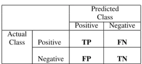
Measuring the predictive performance of a classifier is mainly based on the counts of the cases (learning cases in the training phase and test cases in the test phase) correctly and incorrectly predicted by the classifier. These counts are organized in a tabular structure known as a confusion matrix, as represented in Table I. The entries of the confusion matrix are defined as follows:

TP The count of cases that belong to the positive class and are predicted as positive (true positives).

FP The count of cases that belong to the negative class and are predicted as positive (false positives).

TABLE I CONFUSIONMATRIX. Predicted Class Positive Negative Actual Class Positive TP FN Negative FP TN

TN The count of cases that belong to the negative class and are predicted as negative (true negatives).

FN The count of cases that belong to the positive class and are predicted as negative (false negatives).

SM The total count of cases (TP + FP + TN + FN). The confusion matrix is computed for classification model M using the training set D. Various classification quality evaluation measures can be formulated using the elements of the confusion matrix. The following presents the 7 confusion matrix-based measures investigated in our work.

1) Accuracy(Equation 3) - The baseline measure which is used in the original Ant-Tree-MinerM [7] to evaluate the candidate constructed multi-tree models. Accuracy measures the ratio of the count of correctly classified cases (TP + TN) over the sum of counts of all the cases.

Accuracy= T P+T N

SM (3)

2) F-measure(Equation 5) - Widely used in the context of information retrieval and text classification systems. It calculates a harmonic mean between precision and recall:

P recision= T P

T P+F P Recall= T P

T P +F N (4)

and

F−measure=2·P recision·Recall

P recision+Recall (5)

3) Sensitivity × Specificity(Equation 6) - Sen-sitivity measures the ratio of the count of true positives to the count of all the positive cases, and specificity measures the ratio of the count of true negatives to the count of all the negative cases.

Sensitivity×Specif icity= T P T P +F N ·

T N T N+F P

(6) 4) Jaccard Coefficient (Equation 7) - It calculates the similarity between sample sets. In the classification context, it measures the accuracy only with respect to the true positive count, neglecting the true negatives.

J accard= T P

T P +F P+F N (7)

5) M-estimate(Equation 8) - a parametric function with parameterm:

M−estimate= T P +m· T P SM

We set m to 22.4 as recommended by Janssen and F¨urnkranz in [25].

6) Kappa (Equation 9) - Kappa Statistic, a well-known predictive effectiveness measure, compares the accuracy of the system to the accuracy of a random system. Total accuracy is an observational probability of agreement and random accuracy is a hypothetical expected probability of agreement under an appropriate set of baseline con-straints.

Kappa=Accuracy−RandomAccuracy 1−RandomAccuracy (9)

where

RandomAccuracy=

(T N+F P)·(T N+F N)+(F N+T P)·(F P+T P)

(SM)2 (10)

7) Kl¨osgen (Equation 11) - A parameteric function with parameterω. Whenω = 0, the measure acts as precision (Equation 4). Asωincreases the measure acts in a manner similar to recall (Equation 4). The transition from one to the other is not linear, and asωincreases further it starts acting as coverage. Klosgen= T P+F P SM ω . T P T P+F P − T P+F N SM (11) We used an ω value of 0.43 in our experiments, as recommended by Janssen and F¨urnkranz in [25]. In addition to the confusion matrix-based measures, we used three more classification quality measures that are based on the probability of the classified class. In more details, let m

denote the number of classes,cˆdenote the true (correct) class for a given case x, and c denote the class that is predicted by the classification modelM. The output of the classifier is an m-dimensional probability vector p1, p2, . . . , pm. Hence, the predicted class c will be the labelk of the output of the model M with the highest probability scorepk. We will use the notationf(M|x)to refer to the value of the classification measuref onMgiven casex.

8) Class Probability Error (CPE), also known as Probabilistic Accuracy (Equation 12) - This is a probabilistic alternative to the accuracy measure. For a given casex,

CP E(M|x) = 1−pˆc (12)

CPE computes the difference between the actual (ideal) probability value (1.0) and the predicted probabiliy pˆc

of the correct class ˆc. Hence, CPE favours models that correctly classify the cases with higher probability. This is unlike Accuracy, which counts any classified case with probability of 0.5 or higher for the true class as a true positive.

The pheromone amount to be deposited is based on the evaluation of the entire training set:

QCP E(M|D) = 1− 1 |D|

X

x∈D

CP E(M|x) (13)

9) Mean Squared Error (Equation 14) - MSE is an-other widely used error measure. For a given pattern x:

M SE(M|x) = (1−pc)ˆ2+

m X

k:k6=ˆc

(pk)2 (14) MSE computes the mean squared difference between the predicted probability of each class and its actual (ideal) probability value. For the correct class pˆc, the

ideal probability value is 1.0, while it is 0.0 for the other classes. Note that not only does M SE favour the models that produce a higher probability for the true class, but it also favours the models that produce the lowest probabilities for the other classes.

The pheromone amount to be deposited is based on the evaluation of the entire training set, as follows:

QM SE(M|D) = 1− 1 |D| X x∈D M SE(M|x) (15) 10) Bayesian Information Reward (Equation 16) -For a given pattern x, we use a variation of Bayesian Information RewardBIR, defined as:

BIR(M|x) = 1 m m X c=1 IRc(M|x) (16) where IRc(M|x) = ( 1−log (pc) log (p0 c) if c= ˆc (reward) log (1−pc) log (1−p0 c) if c6= ˆc (penalty) (17) wherep0crepresents the prior probability of classc, which

is the ratio of the number of cases in the learning set with class labelc to the total number of cases in the learning set, andm is the total number of the classes. Note that the first branch in the conditional Equation (17) is the reward value, where the predicted class cis the same as the true (correct) classˆc, while the second branch is the penalty value, where the predicted c is not the same as the true classˆc.

Not only does the Bayesian Information Reward measure take into account the true class pˆc, it also accounts for

the prior probability p0_c of the predicted class in the dataset. This makes BIR more robust to class imbalance situations, where one (or more) class values have high occurrence in a given dataset compared to the other values. That is, the lower the frequency of the correctly predicted class in the dataset, the higher the reward. Similarly, the higher the frequency of the misclassified class in the dataset, the higher the penalty.

The pheromone amount to be deposited is based on the evaluation of the entire training set,

QBIR(M|D) = 1 |D|

X

x∈D

[φ1+BIR(M|x)/φ2] (18) where the parameters φ1 and φ2 are used to adjust the actual amount of pheromone to be deposited. The first

parameter makes sure that theQBIRvalue is greater than 0, while the second parameter scales theQBIRvalue. In our experiments, we set φ1=φ2= 50/m.

It is crucial to emphasize that there are two different quality evaluation operations. The first is the one used in the testing phase to evaluate the classification quality of the final output classifier on a test set unseen during training, which is fixed and used to evaluate several algorithms or several variations of an algorithm. The second is the one used during the training phase for evaluating each candidate classifier constructed by an ant on a validation set.

Candidate solutions are evaluated during the training phase to perform pheromone update for guiding the search to build a high quality classifier as a final output. In the experiments, the former is fixed to Accuracyin the testing phase, while the latter used the various aforementioned measures in the training phase to examine their effectiveness with respect to maximizing the Accuracy test measure. The next section describes the experimental methodology in detail.

V. EXPERIMENTALRESULTS

In our experiments, we modify Ant-Tree-MinerM in two ways. First, We remove the heuristic component from the probabilistic state transition formula. The reason behind this is to isolate the effect of the quality measure and to make sure that only the evaluation measure will affect the ants’ de-cisions and guide the search through the pheromone amounts deposited. Second, we only perform the pruning operation on the final converged-on solution, rather than on each candidate solution, in order to reduce the algorithm’s computational time and again to amplify the effect of the quality measures being compared.

The performance of classification quality measures was evaluated using 40 public-domain datasets from the well-known UCI (University of California at Irvine) dataset repos-itory [8]. The parameter settings used in our experiments are the default values used in [6].

The experiments were carried out using a well-known strat-ified 10-fold cross-validation procedure [1]. This means that each dataset is divided into ten mutually exclusive partitions (folds), with roughly the same class distribution in each partition. Then, the algorithm is run ten times, where each time a different partition is used as the test set and the other nine partitions are collectively used as the training set. The predictive performance reported for each evaluation measure is computed as the average value of the Accuracy on the test set across the runs of the 10 folds.

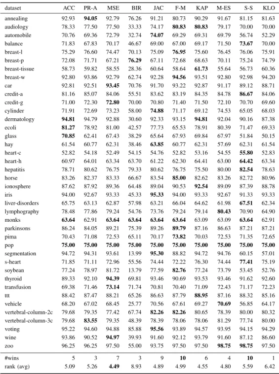
Table II reports the test set predictive accuracy results for Ant-Tree-MinerML for the 10 quality evaluation measures described in Section IV: Accuracy (ACC), Probabilistic Accuracy (PR-A), Mean Squared Error (MSE), Bayesian Information Reward (BIR),Jaccard(JAC),F-measure(F-M),Kappa(KAP), M-estimate(M-ES),Sensitivity-Specificity (S-S), and Kl¨osgen(KLO). For each dataset, the average test set accuracy, aggregated over the 10 cross-validation folds,

is reported for each measure; the highest-accuracy achieved for each dataset is shown in boldface. The penultimate row of the table reports a count of the number of datasets for which each measure achieved the highest accuracy, and the last row reports the average rank of each measure. To obtain the average rank, the ten measures are first ranked for each dataset individually, with the best measure being given a rank of 1, and the worst a rank of 10. In the case of ties, the tied measures are given the average of the spanned ranks. Finally, the ranks are averaged over the datasets to obtain the overall average ranks.

As the table indicates, the best average rank was obtained by Mean Squared Error, with an average rank of 4.49 and the best accuracy in 7 datasets, followed in second-place by Kappa with a rank of 4.55 and the best accuracy in 6 datasets, then in third-place by M-estimate with a rank of 4.80 and the best accuracy in 4 datasets. In fourth-place was Jaccard with an average rank of 4.89 and the best accuracy in 9 datasets, followed by F-measure in fifth-place with a rank of 4.99 and the best accuracy in 10 datasets. In sixth-place was Accuracy(the original quality evaluation measure of Ant-Tree-MinerML) with a rank of 5.09 and the best accuracy in 5 datasets, followed in seventh-place byProbabilistic Accuracywith a rank of 5.26 and the best accuracy in 3 datasets, then in eighth-place by Sensitivity-Specificity with a rank of 5.59 and the best accuracy in 10 datasets. In the last two places were Kl¨osgen with an average rank of 6.42 and the best accuracy in a single dataset, andBayesian Information Reward with a rank of 8.93 and the best accuracy in 3 datasets.

Table IV reports the results of applying a Friedman test with the Holmpost hoctest at the coventional 0.05 threshold to the results of Table II, usingMean Squared Error(the measure with the best average rank) as the control measure. The Friedman statistic χ2_F is determined to be 69.28 with 9 degrees of freedom, corresponding to a p value of 7.0E-11. Thus, we can reject the null hypothesis and proceed with the post hoc tests. For each measure, the second column of the table reports the average rank, the third column reports the

pvalue of the statistical test when the measure is compared to the control measure, and the last column reports the Holm critical value. Statistically significant p values are shown in boldface. The table indicates thatMean Squared Erroris significantly better than two of the other measures:Kl¨osgen, andBayesian Information Reward.

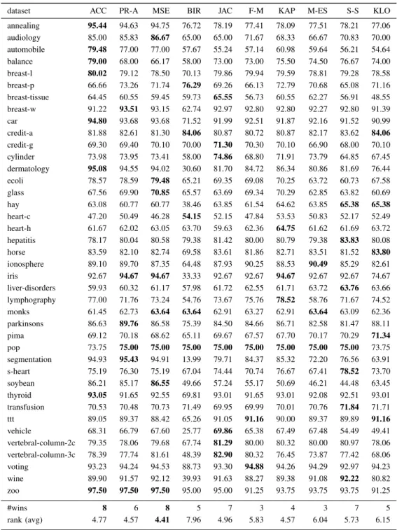
Table III reports the test set predictive accuracy results for Ant-Tree-MinerMI for the same 10 quality evaluation measures, and follows the format of Table II. We can see that there are many similarities, but also a few differences between the pattern of results for Ant-Tree-MinerMI and Ant-Tree-MinerML. For Ant-Tree-MinerMI, the highest average rank was again obtained byMean Squared Error, with an average rank of 4.41 and the best accuracy on 8 datasets. The second-best average rank was a tie between Probabilistic Accuracy, which had a rank of 4.57 and the best accuracy

TABLE II

TEST SET PREDICTIVE ACCURACY(%)FOR EACH OF THE QUALITY MEASURES FORANT-TREE-MINERML.

dataset ACC PR-A MSE BIR JAC F-M KAP M-ES S-S KLO annealing 92.93 94.05 92.79 76.26 91.21 80.73 90.29 91.67 81.15 81.63 audiology 78.33 77.50 77.50 33.33 74.17 80.83 80.83 79.17 70.00 70.00 automobile 70.76 69.36 72.79 32.74 74.07 69.29 69.31 69.79 56.74 52.29 balance 71.83 67.83 70.17 46.67 69.00 67.00 69.17 71.50 73.67 70.00 breast-l 75.29 76.60 74.47 70.13 75.09 76.95 75.60 76.45 76.06 75.91 breast-p 72.08 71.71 67.21 76.29 67.11 72.68 68.63 70.11 75.24 74.79 breast-tissue 58.73 59.82 58.55 28.36 60.64 58.64 61.73 55.64 56.73 60.36 breast-w 92.80 93.86 92.79 62.74 92.28 94.56 93.51 92.80 92.98 94.20 car 92.81 92.51 93.45 70.76 91.70 93.22 92.87 91.17 89.12 88.71 credit-a 81.16 85.07 84.06 55.51 83.62 83.19 84.35 84.78 86.67 84.06 credit-g 71.00 72.30 72.80 70.00 70.80 71.40 71.50 72.10 70.70 69.60 cylinder 71.91 72.69 73.23 58.00 74.88 71.17 69.12 74.53 65.05 68.03 dermatology 94.81 94.79 92.88 30.60 92.33 93.15 94.81 92.04 90.16 87.38 ecoli 81.27 78.92 81.00 42.57 77.73 65.53 78.91 80.39 71.47 69.33 glass 70.85 62.41 67.43 38.29 65.64 67.93 69.84 67.97 51.84 50.15 hay 61.54 60.77 62.31 38.46 63.85 60.77 62.31 57.69 62.31 61.54 heart-c 52.82 54.18 52.49 54.15 54.76 52.82 53.16 54.55 55.80 52.83 heart-h 60.97 64.01 63.34 63.70 61.22 62.30 64.41 63.00 64.42 63.34 hepatitis 78.71 80.62 76.75 79.33 80.62 76.75 75.50 80.00 82.54 78.63 horse 83.26 82.37 83.33 66.67 83.54 85.00 82.62 83.26 82.72 80.96 ionosphere 87.62 87.92 89.36 64.48 89.04 90.53 92.54 89.09 87.39 88.78 iris 94.00 92.67 93.33 45.33 95.33 94.00 93.33 92.67 91.33 93.33 liver-disorders 65.75 63.13 62.87 57.98 63.21 66.04 64.62 61.98 67.51 62.34 lymphography 78.48 77.86 79.24 54.76 73.76 79.24 79.14 80.43 70.90 64.90 monks 63.64 62.91 63.64 63.64 63.64 63.64 63.09 63.09 63.64 62.91 parkinsons 86.24 84.05 89.21 75.39 89.26 89.79 87.16 86.63 87.21 87.21 pima 70.43 71.08 72.53 65.11 70.17 73.82 70.03 72.53 71.35 72.65 pop 75.00 75.00 75.00 75.00 75.00 75.00 75.00 75.00 75.00 75.00 segmentation 94.72 94.31 93.61 13.99 95.30 88.82 94.72 94.76 60.15 57.01 s-heart 71.85 71.11 72.96 55.56 74.44 72.22 76.30 74.44 77.41 75.19 soybean 77.24 78.97 81.72 13.79 77.59 82.76 77.24 73.79 53.45 52.76 thyroid 89.33 92.10 94.39 69.81 93.46 90.69 93.53 93.46 91.62 92.60 transfusion 69.38 71.46 73.14 71.74 70.81 70.40 71.09 72.43 71.17 72.23 ttt 88.42 87.47 88.21 65.26 86.63 87.79 88.95 87.16 88.32 85.16 vehicle 68.20 67.02 68.45 25.77 70.56 67.61 69.27 70.69 56.85 64.17 vertebral-column-2c 79.68 79.35 77.42 67.74 82.26 82.26 80.65 78.39 80.00 80.32 vertebral-column-3c 79.68 83.55 79.35 48.39 78.39 78.06 78.06 81.29 77.74 80.00 voting 95.22 94.60 94.88 85.88 95.56 93.89 94.57 93.95 94.15 94.29 wine 93.86 90.52 94.97 39.93 91.60 92.12 93.79 91.60 87.12 86.60 zoo 96.25 96.25 97.50 55.00 93.75 97.50 97.50 98.75 98.75 97.50 #wins 5 3 7 3 9 10 6 4 10 1 rank (avg) 5.09 5.26 4.49 8.93 4.89 4.99 4.55 4.80 5.59 6.42

on 6 datasets, and Kappa which had the same rank and the best accuracy on 4 datasets. It is interesting that Kappaalso had the second-best ranking for Ant-Tree-MinerML.

In fourth-place was Accuracy with a rank of 4.77 and the best accuracy on 8 datasets, followed in fifth-place by Jaccard with a rank of 4.96 and the best accuracy on 7 datasets. In sixth-place wasSensitivity-Specificity with a rank of 5.73 and the best accuracy on 7 datasets, followed in seventh-place by F-measure with a rank of

5.83 and the best accuracy on 3 datasets. In eighth-place was M-estimatewith a rank of 6.04 and the best accuracy on 3 datasets, followed in ninth-place byKl¨osgenwith a rank of 6.15 and the best accuracy on 5 datasets. Finally, in last place was Bayesian Information Reward with a rank of 7.96 and the best accuracy on 5 datasets. Interestingly, the two worst-ranked measures are the same for the two algorithms.

Table V reports the results of applying a Friedman test with the Holmpost hoctest at the coventional 0.05 threshold to the

TABLE III

TEST SET PREDICTIVE ACCURACY(%)FOR EACH OF THE QUALITY MEASURES FORANT-TREE-MINERMI.

dataset ACC PR-A MSE BIR JAC F-M KAP M-ES S-S KLO annealing 95.44 94.63 94.75 76.72 78.19 77.41 78.09 77.51 78.21 77.06 audiology 85.00 85.83 86.67 65.00 65.00 71.67 68.33 66.67 70.83 70.00 automobile 79.48 77.00 77.00 57.67 55.24 57.14 60.98 59.64 56.21 54.64 balance 79.00 68.00 66.17 58.00 73.00 73.00 75.50 74.50 76.67 74.00 breast-l 80.02 79.12 78.50 70.13 79.86 79.94 79.59 78.81 79.28 78.58 breast-p 66.66 73.26 71.74 76.29 69.26 66.13 72.79 70.68 65.08 71.16 breast-tissue 64.45 60.55 59.45 59.73 65.55 56.73 60.55 62.27 56.91 48.55 breast-w 91.22 93.51 93.15 62.74 92.97 92.80 92.80 92.27 92.80 91.39 car 94.80 93.68 93.68 71.52 91.99 92.51 91.87 92.16 91.52 90.99 credit-a 81.88 82.61 81.30 84.06 80.87 80.72 80.87 82.17 83.62 84.06 credit-g 69.30 69.40 70.10 70.00 71.30 70.30 70.10 66.90 68.00 70.10 cylinder 73.98 73.95 73.41 58.00 74.86 68.80 71.91 73.79 64.85 67.45 dermatology 95.08 94.55 94.02 30.60 81.70 84.72 86.34 80.86 81.69 76.44 ecoli 78.57 78.59 79.48 65.21 69.35 69.08 70.25 63.72 60.73 67.58 glass 67.56 69.90 70.85 65.57 63.69 69.34 70.29 62.85 63.82 60.69 hay 63.08 60.77 60.77 38.46 63.85 61.54 64.62 63.85 65.38 65.38 heart-c 47.20 50.49 46.28 54.15 52.15 47.84 53.53 50.83 52.17 52.49 heart-h 61.67 62.02 63.05 63.70 59.63 62.36 64.75 61.62 61.69 63.72 hepatitis 78.17 80.04 80.58 79.38 81.42 80.00 80.79 79.38 83.83 80.08 horse 83.59 82.10 82.74 69.58 83.61 81.86 82.71 83.51 81.52 83.80 ionosphere 89.10 89.70 87.35 64.48 87.93 90.25 88.53 90.49 85.29 82.61 iris 92.67 94.67 94.67 33.33 92.67 92.67 94.67 92.67 92.67 74.67 liver-disorders 59.93 60.32 61.17 57.98 61.72 62.55 61.71 63.72 63.76 63.66 lymphography 77.00 71.76 73.24 54.76 73.67 75.76 78.52 58.76 71.67 74.52 monks 61.45 62.73 63.64 63.64 62.91 63.27 62.91 63.64 63.09 62.36 parkinsons 86.63 89.76 86.58 75.39 84.50 84.66 86.71 82.58 81.47 88.11 pima 69.12 70.18 68.62 65.11 69.67 67.57 67.70 70.17 70.29 71.34 pop 73.75 75.00 75.00 75.00 75.00 75.00 75.00 75.00 75.00 73.75 segmentation 94.93 95.43 94.91 13.99 79.71 84.37 85.32 72.20 76.56 63.91 s-heart 75.19 76.30 75.19 67.04 74.44 70.74 76.67 67.41 78.52 73.70 soybean 86.21 85.17 86.55 49.66 57.24 55.17 50.69 46.21 44.48 63.45 thyroid 93.05 91.65 92.55 69.81 93.01 91.65 93.01 92.08 92.51 93.01 transfusion 70.53 70.48 70.73 71.49 69.95 69.99 70.01 70.76 71.84 71.71 ttt 89.05 89.37 88.42 65.26 91.05 91.16 90.00 89.37 89.89 91.16 vehicle 68.31 66.79 67.60 25.77 69.86 65.38 67.49 67.48 54.49 49.41 vertebral-column-2c 79.35 78.06 79.68 67.74 81.29 80.00 80.32 80.00 80.97 78.06 vertebral-column-3c 78.39 77.74 81.61 48.39 82.90 80.32 76.45 73.87 77.42 68.06 voting 93.23 94.24 94.53 88.73 93.30 94.88 94.26 94.29 92.97 94.23 wine 89.90 91.57 92.12 39.93 91.63 88.27 89.38 91.08 92.22 80.82 zoo 97.50 97.50 97.50 95.00 95.00 91.25 93.75 93.75 93.75 91.25 #wins 8 6 8 5 7 3 4 3 7 5 rank (avg) 4.77 4.57 4.41 7.96 4.96 5.83 4.57 6.04 5.73 6.15

results of Table III, again usingMean Squared Error(the measure with the best average rank) as the control measure. The Friedman statistic χ2

F is determined to be 46.43 with 9

degrees of freedom, corresponding to a p value of 5.0E-7. Thus, we can reject the null hypothesis and proceed with the post hoc tests. Table V follows the same format as Table IV and indicates that MSE is significantly better than a single measure: Bayesian Information Reward.

VI. CONCLUDINGREMARKS

Ant-Tree-MinerM is a recently introduced algorithm that employs the ACO meta-heuristic to induce multi-tree classifi-cation models. This paper has explored the effect of using 10 different classification quality measures for evaluating the candidate models constructed by the ants and updating pheromone during the training phase of the ACO algorithm. The effect of using these quality measures in the training phase was assessed according to their effectiveness in producing

TABLE IV

RESULTS OF THEFRIEDMAN TEST WITH THEHOLMpost hocTEST,AT THE 0.05SIGNIFICANCE LEVEL,FOR THE PREDICTIVE ACCURACY RESULTS

REPORTED INTABLEII.

measure rank p Holm

Mean Squared Error(control) 4.49 – –

Kappa 4.55 0.926 0.05 M-estimate 4.80 0.644 0.025 Jaccard 4.89 0.555 0.01666 F-measure 4.99 0.460 0.0125 Accuracy 5.09 0.375 0.01 Probabilistic Accuracy 5.26 0.252 0.00833 Sens.-Spec. 5.59 0.104 0.00714 Kl¨osgen 6.42 0.004 0.00625 BIR 8.93 5.6E-11 0.00555 TABLE V

RESULTS OF THEFRIEDMAN TEST WITH THEHOLMpost hocTEST,AT THE 0.05SIGNIFICANCE LEVEL,FOR THE PREDICTIVE ACCURACY RESULTS

REPORTED INTABLEIII.

measure rank p Holm

MSE(control) 4.41 – – Kappa 4.57 0.810 0.05 Probabilistic Accuracy 4.57 0.810 0.025 Accuracy 4.77 0.592 0.01666 Jaccard 4.96 0.417 0.0125 Sens.-Spec. 5.73 0.053 0.01 F-measure 5.83 0.037 0.00833 M-estimate 6.04 0.016 0.00714 Kl¨osgen 6.15 0.010 0.00625 BIR 7.96 1.6E-7 0.00555

classifiers with a high predictive performance in the testing phase, using Accuracy as a fixed predictive performance evaluator.

Empirical evaluation on 40 UCI datasets has shown that the performance of different quality measures varies substan-tially across different datasets. However, theMean Squared ErrorandKappameasures obtained the best overall average predictive performance, while Bayesian Information Reward and Kl¨osgen obtained the worst overall average predictive performance. One possible research direction is to use an ensemble of several quality measures in the same learning procedure, which is left for future work.

ACKNOWLEDGMENT

Partial support of a grant from the Brandon University Research Council is gratefully acknowledged.

REFERENCES

[1] I. H. Witten, E. Frank, and M. A. Hall,Data Mining: Practical Machine Learning Tools and Techniques. San Francisco, CA, USA: Morgan Kaufmann, 2010.

[2] J. Han, M. Kamber, and J. Pei,Data Mining: Concepts and Techniques. San Francisco, CA, USA: Morgan Kaufmann, 2011.

[3] J. Quinlan,C4.5: Programs for Machine Learning. San Francisco, CA, USA: Morgan Kaufmann, 1993.

[4] L. Breiman, J. Friedman, R. Olshen, and C. Stone,Classification and Regression Trees. New York, NY, USA: Chapman & Hall, 1984. [5] M. Dorigo and T. St¨utzle,Ant Colony Optimization. Cambridge, MA,

USA: MIT Press, 2004.

[6] F. E. B. Otero, A. A. Freitas, and C. G. Johnson, “Inducing decision trees with an ant colony optimization algorithm,” Applied Soft Computing, vol. 12, no. 11, pp. 3615–3626, 2012.

[7] K. M. Salama and F. E. Otero, “Learning multi-tree classification models with ant colony optimization,” inProceedings International Conference on Evolutionary Computation Theory and Applications (ECTA-2014), 2014.

[8] A. Asuncion and D. Newman, “University of California Irvine Machine Learning Repository,” 2007. [Online]. Available: http: //www.ics.uci.edu/∼_{mlearn/MLRepository.html}

[9] K. Salama, A. Abdelbar, and I. Anwar, “Data reduction for classification with ant colony algorithms,”Intelligent Data Analysis, 2016, to appear. [10] I. M. Anwar, K. M. Salama, and A. M. Abdelbar, “ADR-Miner: An ant-based data reduction algorithm for classification,” inProceedings IEEE Congress of Evolutionary Computation (CEC-2015), 2015, pp. 515–521. [11] ——, “Instance selection with ant colony optimization,” inProceedings INNS Conference on Big Data, ser. Procedia Computer Science, 2015, vol. 53, pp. 248–256.

[12] R. S. Parpinelli, H. S. Lopes, and A. A. Freitas, “Data mining with an ant colony optimization algorithm,”IEEE Transactions on Evolutionary Computation, vol. 6, no. 4, pp. 321–332, 2002.

[13] D. Martens, M. De Backer, R. Haesen, J. Vanthienen, M. Snoeck, and B. Baesens, “Classification with ant colony optimization,” IEEE Transactions on Evolutionary Computation, vol. 11, no. 5, pp. 651–665, 2007.

[14] K. Salama, A. Abdelbar, and A. Freitas, “Multiple pheromone types and other extensions to the Ant-Miner classification rule discovery algorithm,”Swarm Intelligence, vol. 5, no. 3-4, pp. 149–182, 2011. [15] K. Salama, A. Abdelbar, F. Otero, and A. Freitas, “Utilizing multiple

pheromones in an ant-based algorithm for continuous-attribute classi-fication rule discovery.” Applied Soft Computing, vol. 13, no. 1, pp. 667–675, 2013.

[16] F. Otero, A. Freitas, and C. Johnson, “A new sequential covering strategy for inducing classification rules with ant colony algorithms,” IEEE Transactions on Evolutionary Computation, vol. 17, no. 1, pp. 64–76, 2013.

[17] F. Otero and A. Freitas, “Improving the interpretability of classification rules discovered by an ant colony algorithm,” inProceedings Genetic and Evolutionary Computation Conference (GECCO-2013), 2013, pp. 73–80.

[18] K. Salama and A. Abdelbar, “Learning neural network structures with ant colony algorithms,”Swarm Intelligence, 2015, to appear.

[19] A. M. Abdelbar and K. M. Salama, “A gradient-guided ACO algorithm for neural network learning,” inProceedings IEEE Swarm Intelligence Symposium, 2015, to appear.

[20] A. Abdelbar, I. El-Nabarawy, D. C. Wunch, and K. M. Salama, “Ant colony optimization applied to the training of a high order neural net-work with adaptable exponential weights,” inApplied Artificial Higher Order Neural Networks for Control and Recognition, M. Zhang, Ed. IGI Global Press, 2016, to appear.

[21] K. Salama and A. Freitas, “Learning Bayesian network classifiers using ant colony optimization,”Swarm Intelligence, vol. 7, no. 2-3, pp. 229– 254, 2013.

[22] ——, “Ant colony algorithms for constructing Bayesian multi-net clas-sifiers,”Intelligent Data Analysis, vol. 19, no. 2, pp. 233–247, 2015. [23] ——, “Clustering-based Bayesian multi-net classifier construction with

ant colony optimization,” inIEEE Congress on Evolutionary Computa-tion (CEC-2013), 2013, pp. 3079–3086.

[24] ——, “Extending the ABC-Miner Bayesian classification algorithm,” in Proceedings Sixth International Workshop on Nature Inspired Co-operative Strategies for Optimization (NICSO-2013), ser. Series in Computational Intelligence, vol. 512. Berlin: Springer, 2013, pp. 1–12. [25] F. Janssen and J. Furnkranz, “On the quest for optimal rule learning