Portland State University
PDXScholar
Dissertations and Theses Dissertations and Theses
Fall 11-6-2018
Ensemble Data Assimilation for Flood Forecasting in Operational
Settings: from Noah-MP to WRF-Hydro and the National Water
Model
Mahkameh Zarekarizi Portland State University
Let us know how access to this document benefits you.
Follow this and additional works at:https://pdxscholar.library.pdx.edu/open_access_etds
Part of theCivil and Environmental Engineering Commons, and theHydrology Commons
This Dissertation is brought to you for free and open access. It has been accepted for inclusion in Dissertations and Theses by an authorized administrator of PDXScholar. For more information, please contactpdxscholar@pdx.edu.
Recommended Citation
Zarekarizi, Mahkameh, "Ensemble Data Assimilation for Flood Forecasting in Operational Settings: from Noah-MP to WRF-Hydro and the National Water Model" (2018).Dissertations and Theses.Paper 4651.
Ensemble Data Assimilation for Flood Forecasting in Operational Settings: From Noah-MP to WRF-Hydro and the National Water Model
by
Mahkameh Zarekarizi
A dissertation submitted in partial fulfillment of the requirements for the degree of
Doctor of Philosophy in
Civil and Environmental Engineering
Dissertation Committee: Hamid Moradkhani, Chair
Dacian Daescu Gwynn Johnson
Paul Loikith
Portland State University 2018
i
Abstract
The National Water Center (NWC) started using the National Water Model (NWM) in 2016. The NWM delivers state-of-the-science hydrologic forecasts in the nation. The NWM aims at operationally forecasting streamflow in more than 2,000,000 river reaches while currently river forecasts are issued for 4,000. The NWM is a specific configuration of the community WRF-Hydro Land Surface Model (LSM) which has recently been introduced to the hydrologic community. The WRF-Hydro model, itself, uses another newly-developed LSM called Noah-MP as the core hydrologic model. In WRF-Hydro, Noah-MP results (such as soil moisture and runoff) are passed to routing modules. Riverine water level and discharge, among other variables, are outputted by WRF-Hydro. The NWM, WRF-Hydro, and Noah-MP have recently been developed and more research for operational accuracy is required on these models. The overarching goal in this dissertation is improving the ability of these three models in simulating and forecasting hydrological variables such as streamflow and soil moisture. Therefore, data assimilation (DA) is implemented on these models throughout this dissertation. State-of-the art DA is a procedure to integrate observations obtained from in situ gages or remotely sensed products with model output in order to improve the model forecast. In the first chapter, remotely sensed satellite soil moisture data are assimilated into the Noah-MP model in order to improve the model simulations. The performances of two DA techniques are evaluated and compared in this chapter. To tackle the computational burden of DA, Massage Passing Interface protocols are used to augment the
ii
computational power. Successful implementation of this algorithm is demonstrated to simulate soil moisture during the Colorado flood of 2013. In the second chapter, the focus is on the WRF-Hydro model. Similarly, the ability of DA techniques in improving the performance of WRF-Hydro in simulating soil moisture and streamflow is investigated. The results of chapter 2 show that the assimilation of soil moisture can significantly improve the performance of WRF-Hydro. The improvement can reach 58% depending on the study location. Also, assimilation of USGS streamflow observations can improve the performance up to 25%. It was also observed that soil moisture assimilation does not affect streamflow. Similarly, streamflow assimilation does not improve soil moisture. Therefore, joint assimilation of soil moisture and streamflow using multivariate DA is suggested. Finally, in chapter 3, the uncertainties associated with flood forecasting are studied. Currently, the only uncertainty source that is taken into account is the meteorological forcings uncertainty. However, the results of the third chapter show that the initial condition uncertainty associated with the land state at the time of forecast is an important factor that has been overlooked in practice. The initial condition uncertainty is quantified using the DA. USGS streamflow observations are assimilated into the WRF-Hydro model for the past ten days before the forecasting date. The results show that short-range forecasts are significantly sensitive to the initial condition and its associated uncertainty. It is shown that quantification of this uncertainty can improve the forecasts by approximately 80%. The findings of this dissertation highlight the importance of DA to extract the information content from the observations
iii
and then incorporate this information into the land surface models. The findings could be beneficial for flood forecasting in research and operation.
iv
Dedication
To Mahasti and Faramarz
Mom, Dad, I lived my life in the past four years to make every second of not seeing you worth living. I failed a lot and I wanted to give up so many times. However, whenever I asked myself “Is that why I left my home?” I stood back up and worked even harder. You dedicated your lives to me and dedicating this book to you is the least I could do.
v
Acknowledgments
I would like to express my deepest gratitude to my advisor, Dr. Hamid Moradkhani. He taught me a lot more than hydrology and data assimilation. I thank him for all the opportunities and supports he provided. He helped me become the researcher, I am today.
I thank my dissertation committee, Dr. Gwynn Johnson, Dr. Paul Loikith, and Dr. Dacian Daescu for offering their time to review my dissertation and providing me with their valuable comments.
Special thanks to Dr. Ali Ahmadalipour for reviewing and editing my dissertaion. His comments helped me improve the quality of this dissertation.
I thank Dr. Hongxiang Yan, former PSU student and my mentor for teaching me many things I could not imagine to learn by myself. He was always helpful and available whenever I needed him even after he left PSU.
I thank William Garrick, the Research Computing Manager in the Office of Information Technology, Portland State University. He truly helped me whenever I needed help with the Coeus cluster. He always immediately replied my emails no matter if it was after hours or holidays. A significant portion of this dissertation could not happen without his assistance.
I deeply thank Roxanne Treece, Assistant Director of Graduate Academic Services for supporting me during the graduation process. Her assistance made my
vi
transition after Ph.D. much easier. Also, thanks to CEE faculty and staff especially Dr. Chris Monsere, Megan Falcone and Samantha Parsons for their consistent help in my program.
I thank NWC, WRF-Hydro, and CUAHSI teams for hosting me in NWC summer school and WRF-Hydro training workshop. They patiently answered my questions when I was learning about the NWM, and they made data required for this dissertation available for me. Special thanks to Dr. David Gochis and Dr. Arezoo RafieeiNasab.
I thank my dearest colleagues and friends Dr. Arun Rana, Dr. Ali Ahamdalipour and Sepideh Khajehei. Arun was my mentor when I had just started my program in PSU. Ali always encouraged and supported me. Sepideh was always there for me no matter if I was in Portland or Alabama. I thank everyone in the “Remote Sensing and Water Resources” lab, especially Maysoun Hameed.
I appreciate all the support from my beloved partner, Hamed who unconditionally supported me in every moment of happiness or frustration. He kept me inspired and motivated, and he always believed in me even when I did not.
Last but not least, my warm acknowledgments to my parents and Ardeshir, my only and favorite brother for unconditionally loving me and supporting me when I decided to leave them in pursuit of my dreams.
vii Table of Contents Abstract ... i Dedication ... iv Acknowledgments... v List of Tables ... xi
List of Figures ... xii
List of Abbreviations ... xviii
1 Motivation ... 1
2 Data Assimilation to enhance Noah-MP soil moisture predictions ... 7
2.1 Abstract………. ... 7
2.2 Highlights……….. ... 8
2.3 Introduction ... 8
2.4 Study area and data ... 12
2.4.1 Colorado Front Range and the 2013 flood ... 12
2.4.2 Satellite soil moisture observations ... 13
2.4.3 Meteorological forcing... 15
2.5 Noah-MP Land Surface Model ... 17
2.6 Methodology ... 24
2.6.1 Data Assimilation... 24
2.6.1.1 Particle Filter ... 24
2.6.1.2 Ensemble Kalman Filter ... 28
viii
2.6.3 Performance assessment ... 35
2.6.4 Characterization of uncertainties ... 35
2.7 Model setup and pre-processing ... 36
2.7.1 Re-gridding the forcing inputs ... 36
2.7.2 Domain files ... 38
2.8 Results ... 41
2.8.1 Example: A simple model run results ... 41
2.8.2 Synthetic Study ... 44
2.8.3 Real Study ... 54
2.9 Summary ……….59
2.10 Conclusion, discussion, and future work ... 61
3 A Multivariate Ensemble data assimilation in the WRF-Hydro: Potential DA Integration to the National Water Model ... 63
3.1 Abstract ... 63
3.2 Highlights ... 64
3.3 Introduction ... 64
3.4 Study area and data ... 71
3.4.1 Study area ……….71 3.4.2 Streamflow ... 76 3.4.3 Atmospheric forcings ... 76 3.5 Methodology ... 77 3.5.1 WRF-Hydro ... 77 3.5.2 Data Assimilation... 80 3.5.3 High-performance computing ... 80
ix
3.5.4 Performance measures ... 81
3.6 Results ... 82
3.6.1 LSM setup and preprocessing ... 83
3.6.2 Characterizing the uncertainties ... 84
3.7 Synthetic study ... 84
3.7.1 Univariate soil moisture assimilation... 85
3.7.2 Univariate streamflow assimilation ... 97
3.7.3 Multivariate assimilation of soil moisture and streamflow... 105
3.7.4 Summary of the performance measures ... 112
3.8 Real study……... 113
3.9 Conclusion and discussion ... 117
4 Improved National Water Model forecasts based on Ensemble data assimilation ... 121
4.1 Abstract ... 121
4.2 Introduction ... 122
4.3 Study area and data ... 128
4.4 Methodology ... 128
4.4.1 National Water Model... 128
4.4.2 Data assimilation ... 130 4.4.3 High-Performance Computing ... 131 4.4.4 Performance measures ... 131 4.5 Results ... 131 4.5.1 Synthetic study ... 131 4.5.1.1 Short-range forecasts ... 132
x
4.5.1.2 Medium-range forecasts... 134
4.5.1.3 Long-range forecasts ... 136
4.5.2 Real study ... 137
4.6 Conclusion and discussion ... 140
5 Conclusion ... 143
xi
List of Tables
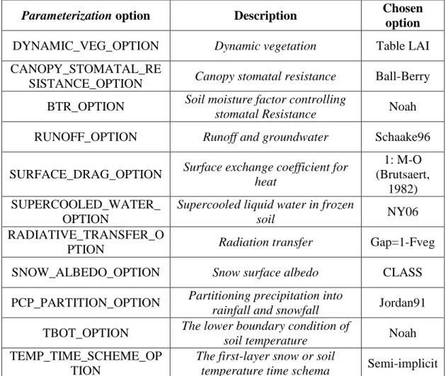
Table 2-1: Noah-MP parameterization options and the selected schemes used in this study ... 40 Table 3-1: USGS gauge information for two study areas in this chapter ... 76 Table 3-2: Univariate synthetic soil moisture assimilation results. The spatial mean of performance measures of OL and DA over the domain in Croton, NY. ... 95 Table 3-3: Univariate synthetic soil moisture assimilation results. The effects of soil moisture assimilation on streamflow are presented. The first two rows indicate the measures for the Huntsville domain and the lower three rows show the measures for the Croton area. OL and DA RMSE, NSE, BIAS, and KGE are shown in the columns. The last column shows NIC, the improvement made by DA over OL. ... 97 Table 3-4: Univariate synthetic streamflow assimilation results. The performances of OL and DA in simulating streamflow are measured by RMSE, BIAS, KGE, and NSE. The first three rows indicate the measures for the Croton domain and the lower two rows show the measures for the Huntsville area. The last column shows NIC, the improvement made by DA over OL. ... 98 Table 3-5: Multivariate synthetic streamflow and soil moisture assimilation results. Comparison of spatially-averaged performance of OL and DA in simulating soil moisture in Croton, NY is performed. ... 111 Table 3-6: Multivariate synthetic streamflow and soil moisture assimilation results. Comparison of performance measures of OL and DA in simulating streamflow in all gages in both watersheds. A better performance is shown in bold. ... 112 Table 3-7: Summary of performance measures in all scenarios. NI indicates no improvement, P25, µ, and P75 indicate the 25th, average, and the 75th spatial percentile.
The first column from left is associated with the scenario of univariate assimilation of soil moisture. The middle column results are related to the univariate assimilation of streamflow, and the third column (on the right) indicates the result of multivariate assimilation of both soil moisture and streamflow. Numbers are in percent. ... 113 Table 3-8: OL and DA root mean square errors and the degree of improvements by DA for the real case study. ... 114
xii
List of Figures
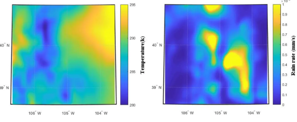
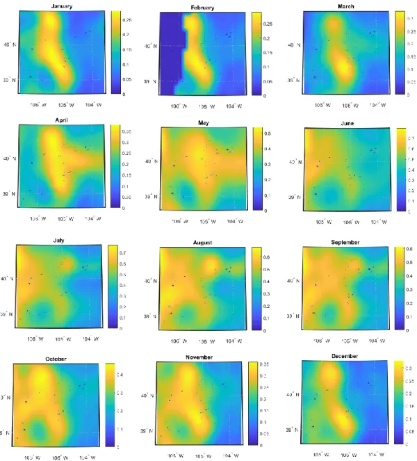
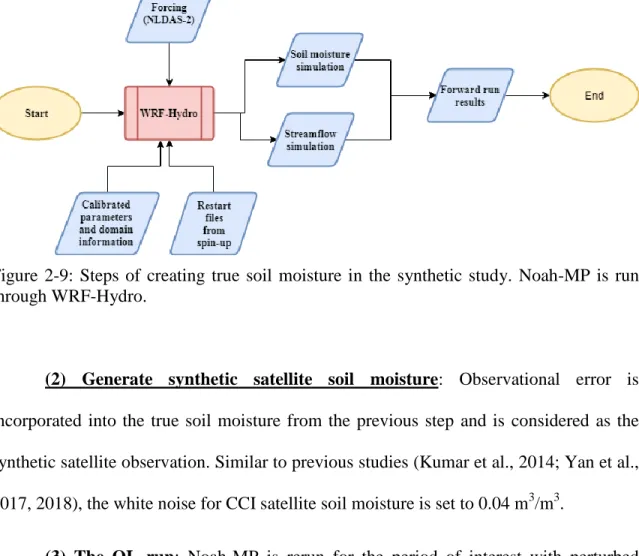
Figure 2-1: Imagery and location of the studied area, Colorado Front Range ... 13 Figure 2-2: Parallel ensemble data assimilation flowchart used in this dissertation ... 34 Figure 2-3: Temperature and rainfall inputs obtained from the NLDAS dataset and mapped over the study area. Both datasets are mapped for September 12, 2018 12:00 PM. ... 37 Figure 2-4: Height (m) as used in the domain file to run the Noah-MP model. ... 38 Figure 2-5: Monthly green fraction fields used as input in the Noah-MP domain file. Data are obtained from the WRF pre-processing tool. ... 39 Figure 2-6: Noah-MP example run results without data assimilation. Spatial variation of simulated runoff on Sep 12, 2013, when rainfall was at the peak. The yellow parts indicate where the water is ponded due to infiltration excess over the urbanized areas .. 43 Figure 2-7: Noah-MP example run results without data assimilation. Spatial variation of simulated soil moisture. The top layer (upper left) is 10 cm, the second layer (top right) is 30 cm, the third layer (bottom left) is 60 cm, and the deep layer (bottom right) layer is 100 cm. ... 43 Figure 2-8: Noah-MP example run results without data assimilation. Temporal variation of soil moisture, averaged over the area, converted to mm in September 2013. ... 44 Figure 2-9: Steps of creating true soil moisture in the synthetic study. Noah-MP is run through WRF-Hydro. ... 45 Figure 2-10: A schematic of synthetic soil moisture assimilation. The upper part shows the generation of the synthetic soil moisture data and the lower part is associated with assimilating the synthetic data. Noah-MP and WRF-Hydro are interchangeable in this figure. ... 47 Figure 2-11: Synthetic experiment results. Surface soil moisture simulations from the forward run (red line) and the open loop run (blue lines). The open loop run is an ensemble of model runs with perturbed forcings. The 50% predictive intervals are shown with dashed lines ... 48 Figure 2-12: Synthetic experiment results. Temporal variation of bias from the PF-MCMC, the EnKF, and the OL runs. In PF and EnKF, similar observations are assimilated. Biases are averaged over the area. The simulation starts on 9/5/2013. ... 49
xiii
Figure 2-13: Synthetic experiment results. Comparison of average biases in the (from left to right) EnKF, the OL, and the PF runs. Biases are spatiotemporally averaged over the domain and over the simulation period (September 2013). ... 50 Figure 2-14: Synthetic experiment results. Spatial variation of biases in the OL (top panel), the OL (middle panel), and the EnKF (bottom panel). Biases are calculated on 9/12/203, at the peak of the rainfall. ... 51 Figure 2-15: Synthetic study results. The degree of improvements achieved by DA. EnKF improvements are mapped on the left and the PF improvements are mapped on the right. The improvements are quantified through Normalized Information Contribution. ... 53 Figure 2-16: Synthetic study results. Comparison of EnKF and PF performances. The performance is quantified by Normalized Information Contribution. Higher positive values indicate the superiority of PF over EnKF and negative values indicate the superiority of EnKF. ... 54 Figure 2-17: Background: Rescaled CCI satellite soil moisture in Colorado Front Range averaged over all hours in September 2013 over the study area. Points: Location of in-situ soil moisture gauges. Stations are labeled with the numbers assigned to stations for the analyses of this chapter. ... 56 Figure 2-18: Real experiment results. Performance evaluation of EnKF (the top panel) and the PF-MCMC (the bottom panel). Performance is quantified by NIC. Positive values show improvements made by DA. Higher values of NIC are associated with higher improvements. The x-axis shows the station number. ... 57 Figure 2-19: Real experiment results. Performance evaluation of PF-MCMC over the EnKF. Performance is quantified by NIC. Positive values show improvements made by PF-MCMC. Higher values of NIC are associated with higher skills of PF-MCMC to EnKF. The x-axis shows the station number. ... 58 Figure 3-1: The location of the study area in Croton, NY. ... 72 Figure 3-2: The elevation of the studied domain in Croton, NY. ... 73 Figure 3-3: The location (the top panel) and elevation (the bottom panel) of the studied area in Huntsville, AL. ... 74 Figure 3-4: Strahler stream order in the high-resolution terrain file of WRF-Hydro model. The red circle indicates the location of the outlet point where USGS measurements are available. ... 75 Figure 3-5: Schematic of WRF-Hydro structure (Gochis et al., 2018) ... 79
xiv
Figure 3-6: The procedure and required files to run the WRF-Hydro model ... 79 Figure 3-7: The algorithm of the parallel data assimilation methodology applied in this chapter. ... 81 Figure 3-8: A schematic of the synthetic study algorithm. In this case, synthetic discharge is assimilated into the model. The other version of this figure, Figure 2-10, shows assimilation of synthetic soil moisture. ... 85 Figure 3-9: Univariate synthetic soil moisture assimilation results. Performance of OL and DA in simulating soil moisture in the Huntsville domain. Performance is measured by RMSE, NSE, KGE, and BIAS. ... 86 Figure 3-10: Univariate synthetic soil moisture assimilation results. Spatial variation of RMSE in Huntsville, AL from the OL run (upper left panel) and from the DA run (upper right panel). In the scatter plot, cells are indicated by points. The 1:1 gray line indicates equal RMSE of OL and DA. The area above the 1:1 line shows the outperformance of DA and the area below the 1:1 line shows the outperformance of OL. ... 88 Figure 3-11: Univariate synthetic soil moisture assimilation results. Spatial variation of NSE in Huntsville, AL from the OL run (upper left panel) and from the DA run (upper right panel). In the scatter plot, cells are indicated by points. The 1:1 gray line indicates equal RMSE of OL and DA. The area above the 1:1 line shows the outperformance of OL and the area below the 1:1 line shows the outperformance of DA. ... 89 Figure 3-12: Univariate synthetic soil moisture assimilation results. Spatial variation of BIAS in Huntsville, AL from the OL run (upper left panel) and from the DA run (upper right panel). In the scatter plot, cells are indicated by points. The 1:1 gray line indicates equal RMSE of OL and DA. The area above the 1:1 line shows the outperformance of DA and the area below the 1:1 line shows the outperformance of OL. ... 90 Figure 3-13: Univariate synthetic soil moisture assimilation results. Spatial variation of KGE in Huntsville, AL from the OL run (upper left panel) and from the DA run (upper right panel). In the scatter plot, cells are indicated by points. The 1:1 gray line indicates equal RMSE of OL and DA. The area above the 1:1 line shows the outperformance of OL and the area below the 1:1 line shows the outperformance of DA. ... 91 Figure 3-14: Univariate synthetic soil moisture assimilation results. Level of improvement by the DA over OL is indicated by NIC. NIC for the Huntsville, AL domain is mapped in the top panel. The histogram of all cells is plotted in the bottom panel. ... 93
xv
Figure 3-15: Univariate synthetic soil moisture assimilation results. Comparisons of OL and DA RMSE (upper left), NSE (upper left), KGE (lower left), and BIAS (lower right) in the Croton, NY area are presented in the scatter plots. ... 95 Figure 3-16: Univariate synthetic soil moisture assimilation results. The degree of improvement made by DA in the Croton, NY area is mapped. In 94.5% of the cells, the NIC is positive (improvements by DA) and in 5.4% of the area, the NIC is negative (degradation from DA). ... 96 Figure 3-17: Univariate synthetic streamflow assimilation results. The effect of streamflow assimilation on soil moisture is evaluated. RMSE (upper left panel), NSE (upper right panel), KGE (lower left panel), and BIAS (lower right panel) are plotted for OL and DA. The bars show the spatially averaged. The study area is Huntsville, AL. . 100 Figure 3-18: Univariate synthetic streamflow assimilation results. Same as Figure 3-17 but for the Croton, NY area. ... 101 Figure 3-19: Univariate synthetic streamflow assimilation results. The effect of streamflow assimilation on soil moisture is evaluated. RMSE (upper left panel), NSE (upper right panel), KGE (lower left panel), and BIAS (lower right panel) are plotted for OL and DA. Points represent grid cells in the area. The gray line is the 1:1 line that indicates the equal performance of OL and DA. The study area is Huntsville, AL. ... 102 Figure 3-20: Univariate synthetic streamflow assimilation results. Improvements of DA over OL in soil moisture simulations in the scenario that univariate streamflow is assimilated at USGS gauges. The study area is Huntsville, AL. The spatial variation of NIC is mapped in the upper panel and the histogram of grid cell NICs is plotted in the bottom. ... 104 Figure 3-21: Multivariate synthetic streamflow and soil moisture assimilation results. OL and DA performance measures for soil moisture simulations in Huntsville, AL. ... 106 Figure 3-22: Multivariate synthetic streamflow and soil moisture assimilation results. Spatial distributions of RMSE, NSE, BIAS, and KGE measures are provided in row 1, 2, 3, and 4, respectively. The left column shows OL and the right column shows the DA. The study area is Huntsville, AL. ... 107 Figure 3-23: Multivariate synthetic streamflow and soil moisture assimilation results. Cell-wise comparisons of OL and DA performance in Huntsville, AL. Dots represent cells in the domain. The gray line is the 1:1 line. ... 109 Figure 3-24: Multivariate synthetic streamflow and soil moisture assimilation results. The degree of improvement of DA over OL for soil moisture simulations as indicated by NIC
xvi
for Huntsville, AL. The spatial distribution of the improvements is shown on the upper panel. The histogram of the values is shown in the lower panel. ... 110 Figure 3-25: Multivariate synthetic streamflow and soil moisture assimilation results. The spatial distribution of NIC as an indication of improvements by DA over OL in simulating soil moisture is mapped. The white cells indicate the water bodies. ... 111 Figure 3-26: Streamflow performance measures of the OL and DA. The blue bars indicate OL and the orange bars indicate DA. KGE and NSE are dimensionless and RMSE is in m3/s ... 115 Figure 3-27: BIAS (in m3/s) in the studied gauges. The DA technique is a univariate EnKF to assimilate streamflow observations. ... 115 Figure 3-28: Comparison of OL, DA and observed streamflow in (1) Huntsville outlet, (2) upstream gauge of Croton, (3) middle gauge of Croton, and (4) outlet gauge in Croton. ... 116 Figure 4-1: Four configurations of the NWM, the data used, and the associated frequencies (adopted from the NWM website at http://water.noaa.gov/about/nwm) ... 129 Figure 4-2: A Schematic of the NWM modules and procedures. ... 130 Figure 4-3: Improvements (as indicated by NIC) by DA as compared to the OL for short-term streamflow forecasts in Huntsville, AL. ... 132 Figure 4-4: Performance measures of the OL and DA short-range predictions at the outlet of the Huntsville, AL area. Forecasts are initialized on 2/10/2018. ... 133 Figure 4-5: Same as Figure 4-4 but for the internal gauge of the same area (short-term forecasts initialized on 2/10/2018. ... 134 Figure 4-6: Medium-range forecast performance of DA as compared to OL indicated by NIC for the Huntsville, AL area. ... 135 Figure 4-7: Performance measures of OL and DA for medium-range forecasts in Huntsville, AL... 136 Figure 4-8: Degree of improvements by DA over OL at the outlet and the internal gauges for long-range forecasts in Huntsville, AL area. ... 137 Figure 4-9: Variation of improvements by DA as opposed to OL with lead-time. Forecasts are initiated on 2/5/2018 before the flood peak at the rising limb of the hydrograph ... 138
xvii
Figure 4-10: DA improvements in short-, medium-, and long-range forecasts. Forecasts are initiated on 2/5/2018 before the flood starts. The lead times are defined in a similar way as the NWM. ... 139 Figure 4-11: Time series of forecasted streamflow in OL and DA initial condition. DA Forecast (the red line) is initiated on 2/5/2018. The blue line indicates the OL forecasts and the black line indicates the observation. ... 140
xviii
List of Abbreviations
CCI………....Climate Change Initiative DA………..………….. Data assimilation
EnKF……….……….... Ensemble Kalman Filter ESA ………..………… European Space Agency LAI………..….. Leaf Area Index
LSM………..……….. Land Surface Model MCMC………...………….. Markov Chain Monte Carlo MPI………..…….. Massage Passing Interface
NASA……….. National Aeronautics and Space Administration
NLDAS……….. North American Land Data Assimilation System
NOAA………..….. National Oceanic and Atmospheric Administration
NWC……….... National Water Center
NWM……….….. National Water Model
NWS……….….. National Weather Service
OL……….. Open Loop
xix
PF……….….. Particle Filter
RFC……….….. River Forecast Center
SMAP………..….. Soil Moisture Active Passive
UNOOSA……….. United Nation’s Office for Outer Space
WRF……….….. Weather Research and Forecast
1
1 Motivation
As the costliest natural hazard, floods have affected 2,490 million people between 1980 and 2004 over the globe (Strömberg, 2007). From 1900 to 2015, the U.S. has had 35,000 disasters out of which 40 percent are floods (Cigler, 2017). Two most recent examples of disasters that led to widespread flood are hurricane Harvey (Omranian et al., 2018) in September 2017 and Hurricane Florence in September 2018. Another example is the 2013 flood in Colorado Front Range that affected 18,000 people with a cost of around $2 billion. This highlights the need for an efficient and effective operational flood forecasting system. Currently, River Forecast Centers (RFCs) are in charge of flood monitoring and forecasting up to a week in advance. There are 13 RFCs in the U.S. including Missouri, North Central, Northeast, Northwest, Ohio, Southeast, West Gulf, Arkansas-Red, Alaska River, Colorado, California-Nevada, Lower Mississippi, and Mid-Atlantic. RFCs are in charge of approximately 4,000 river locations over the U.S. The need for a more comprehensive and process-based forecasting system with a longer lead-time and a better spatial coverage over the U.S., brought the National Water Center (NWC) into operation. The NWC has taken the lead for operational flood forecasting over the U.S. since 2015. The primary model in the NWC is the National Water Model (NWM). With the goal of improving water prediction services in National Oceanic and Atmospheric Administration (NOAA), the NWM started operating in August 2016. The distinct feature of the NWM is that it increases the 4,000 prediction locations to 2,700,000 locations over the Continental United States for streamflow prediction. In
2
addition to streamflow prediction, it simulates hydrological variables such as soil moisture and runoff. These variables are delivered at two spatial resolutions of 1 (km) and 250 (m). Another mission of the NWM is providing hyper-resolution (street-level) water predictions (Deo et al., 2018) for the National Weather Service (NWS) in order to improve decision making (http://water.noaa.gov/about/nwm; accessed on 9/18/2018). This feature is valuable in cases of hurricane-related flooding such as Harvey and Florence. The NWM is run operationally in four configurations including “Analysis and Assimilation”, “Short-Range”, “Medium-Range”, and “Long-Range”. The first run operates every hour and runs the NWM for the past 3 hours for a better estimation of the current land surface states and initializing the next three runs. The second run operates every hour and predicts streamflow and other hydrologic variables for the next 0-18 hours, the third run operates four times a day and issues forecasts up to the next ten days, and the last run, operates daily and issues forecasts for up to 30 days. The NWC has been successful in operationally running the model with high resolution over a large scale, and the quality of forecasts is constantly increasing through research. The NWC encourages research on the NWM by holding summer schools that gather graduate students from all over the nation to develop and work on research projects that directly help improve the model (Afshari et al., 2016; Brazil, 2018; Deo et al., 2018).
The NWM is a specific configuration of the community WRF-Hydro Land Surface Model (LSM) which has recently been introduced to the hydrologic community (Gochis et al., 2015, 2018). The WRF-Hydro model, itself, uses another newly-developed
3
column LSM called Noah-MP (Niu et al., 2011; Yang et al., 2011) as the core hydrologic model. In WRF-Hydro, Noah-MP results (such as soil moisture and runoff) are passed to surface and subsurface routing modules. The results are then passed to a channel routing model. Riverine water level and discharge, among other variables, are outputted by WRF-Hydro.
The Noah-MP and WRF-Hydro models are of particular interest in this dissertation. Previous studies (Lin et al., 2018; Yang et al., 2011; Zhang et al., 2016) had shown the effectiveness of these models in simulating hydrological variables (i.e., soil moisture, runoff, and river discharge); however, they (similar to other LSMs) are subject to uncertainties. These uncertainties are associated with climate change (Ahmadalipour et al., 2017a, 2017c; Barlage et al., 2015; Rana and Moradkhani, 2016), urbanization (Pathiraja et al., 2018a), climate variability (Loikith et al., 2017; Zarekarizi et al., 2017), and model structure and parameterization (Moradkhani et al., 2018; Pathiraja et al., 2016a).
To quantify and reduce uncertainty, Data Assimilation (DA) can be used (Liu and Gupta, 2007; Moradkhani et al., 2005a). Hydrologic DA is a mathematical discipline to integrate land surface model simulations with observations to improve the forecast skills (Chen et al., 2013; Moradkhani et al., 2012, 2005b; Pathiraja et al., 2018a, 2018b; Pathiraja et al., 2016a; Piazzi et al., 2018; Zaitchik et al., 2008). Commonly used DA methods in the hydrologic community are the Ensemble Kalman Filter (EnKF) (Clark et al., 2008), Particle Filter (PF) (Moradkhani et al., 2005; 2012; 2018), and Variational DA
4
(Daescu and Langland, 2017; Hamill and Snyder, 2000; Shaw and Daescu, 2016). EnKF was introduced by Evensen (1994) to build upon the well-known Kalman Filter (Kalman, 1960) and has been used to improve hydrologic modeling and prediction (Clark et al., 2008; Komma et al., 2008; Moradkhani et al., 2005b; Pathiraja et al., 2016a). Even though the EnKF is a statistically optimal estimation of a linear, Gaussian system, its widespread application in non-Gaussian and linear problems, has made this method a popular tool in hydrologic modeling (Maneta and Howitt, 2014; Moradkhani et al., 2005b; Pathiraja et al., 2016a). On the other hand, PF-based methods are not subject to the limitation of the EnKF such as (1) Gaussian assumption of errors in model states and observations, (2) linear updating of model states, and (3) violation of the water balance due to linearly adjusting (updating) the states. In the PF, the water balance is not violated since ensemble members are resampled instead of being adjusted (Moradkhani, 2008). The PF has been used for a variety of purposes from streamflow modeling and prediction (Dechant and Moradkhani, 2011) to extreme drought and flood forecasting (Ahmadalipour et al., 2017b; Yan et al., 2018, 2017). The PF has evolved over time and one of the recent advancements resulted in the Particle Filter Markov Chain Monte Carlo (PF-MCMC) (Andrieu et al., 2010; Moradkhani et al., 2012) and recently to Evolutionary Particle Filter which combines the strengths of PF-MCMC and an Evolutionary optimization, i.e., Genetic algorithm (Abbaszadeh et al., 2018). Yan et al. (2018) employed a parallel PF-MCMC to assimilate remotely sensed soil moisture observations into the Variable Infiltration Capacity (VIC) model. They demonstrated a better drought monitoring skill than currently implemented drought monitoring products. Yan et al.
5
(2017 and 2018) used the PF-MCMC and assimilated satellite soil moisture into the VIC model and combined the results with a multivariate statistical drought forecasting approach showed that initializing the drought forecasting model with updated soil moisture states from DA results in more accurate drought forecasts. They tested their methodology to hindcast the widespread drought of 2012 in the U.S. and showed that with DA, the drought could have been predicted weeks in advance.
Similarly, the goal of this dissertation is to answer this question in the context of flood forecasting. Therefore, the overarching goal of this dissertation is to improve the performance of Noah-MP, WRF-Hydro, and the NWM in simulating and forecasting flood. Specifically, answering the following questions is targeted:
(1) What are the main sources of uncertainty in flood forecasting? How could these sources be quantified? How sensitive are the forecasts to the uncertainties? Is initial condition uncertainty an important source? How long does it take for the system to forget about the initial conditions?
(2) Are DA techniques able to improve the performance of Noah-MP in simulating soil moisture? How well are they able to improve the model? Which DA technique has better performance? How efficient are these methods?
(3) How well are DA techniques able to improve the performance of the WRF-Hydro model? Does assimilation of satellite soil moisture into WRF-WRF-Hydro affect the streamflow simulations? Does assimilation of USGS streamflow observations lead to improved soil moisture simulations?
6
Research and operation could benefit from the outcomes of this dissertation toward improving the skill of current flood forecasting systems while reducing the uncertainties. The outcomes help identify potential additions for future improvements in flood forecasting, especially in the NWM. The assessments provided in this dissertation are important preliminary steps toward a better land surface modeling practice for a better weather prediction skill and more accurate large-scale flood forecasts.
The dissertation is organized as follows: In the second chapter, a literature review on Noah-MP and DA techniques are first provided and then, two experiments are designed and illustrated. The results and implications of these experiments are discussed in the end. In the third chapter, the WRF-Hydro model is targeted. Again, the relevant experiments are designed and the analyses and results are discussed. In the third chapter, initial condition uncertainty in flood forecasting is quantified. Synthetic and real data experiments are elaborated in that chapter and their findings and significance are discussed. The dissertation concludes with an overall summary of the main findings, discussion, and future work.
7
2 Data Assimilation to enhance Noah-MP soil moisture predictions
2.1 Abstract
Noah-MP is a land surface model that has recently attracted attention from the meteorological community because it can be coupled with weather forecasting models such as Weather Research and Forecast (WRF). The ability of the model to accurately simulate soil moisture is of particular interest because soil moisture plays an important role in agriculture productivity and flood/drought prediction. This chapter investigates the possibility to further improve the model’s skill in simulating soil moisture. Besides using a land surface model, soil moisture can be obtained from satellite measurements, and it has been shown that combining remotely-sensed and model-simulated soil moisture through data assimilation (DA) techniques can result in more accurate hydrologic forecasts. In this study, data assimilation methods are evaluated on the Noah-MP model. Particularly, two commonly used techniques, the Ensemble Kalman Filter (EnKF) and Particle Filter Markov Chain Monte Carlo (PF-MCMC) are assessed and compared. Additionally, an algorithm is proposed to handle the computational demand of such a large-scale DA implementation. The algorithm is designed for high-performance computing infrastructure and clusters of computational nodes. The results indicate that the DA successfully improves Noah-MP’s ability in simulating soil moisture. Results of comparing EnKF and PF-MCMC indicate that the PF-MCMC has a higher skill in
8
improving soil moisture. Finally, the proposed parallel algorithm is implemented for simulating soil moisture during the Colorado Front Range flood in 2013.
2.2 Highlights
(1) Two commonly used data assimilation methods, the Ensemble Kalman Filter and Particle Filter Markov Chain Monte Carlo, are successfully implemented on Noah-MP.
(2) Particle Filter DA shows a higher skill in improving Noah-MP’s soil moisture simulations.
(3) A high-performance-computing method is implemented to meet the computational demand.
2.3 Introduction
Noah-MP (Yang et al., 2011) is a Land Surface Model (LSM) that plays an important role in earth system modeling. The water stored in the land during a wet season will eventually return to the atmosphere in the dry season through evapotranspiration (Niu et al., 2011). Noah-MP is capable of modeling this feedback. Soil moisture (the water stored in the land) plays a key role in this feedback because it has a persistence characteristic. This means that the water stored in soil needs weeks or even seasons to evaporate. Therefore, soil moisture can provide information about the future of the atmosphere and is known to affect weather predictability (Niu et al., 2011). On the other hand, it determines onset, duration, and termination of agricultural droughts
9
(Ahmadalipour et al., 2017b; Madadgar and Moradkhani, 2013; Yan et al., 2017; Yan et al., 2018) and it also is one of the important predictands of (flash) floods (Cenci et al., 2017). Previous research (Gao et al., 2015; Martinez et al., 2016; Xia et al., 2017; Zhang et al., 2016) has shown that Noah-MP is significant in simulating soil moisture. For example, Cai et al. (2014a) concluded that Noah-MP has a significant capability in modeling the soil moisture. Also, Yang et al. (2011) studied the performance of soil moisture modeling in Noah-MP as compared with the Noah LSM (the previous version on Noah-MP) and found that Noah-MP improves the simulations.
In addition to land surface modeling of soil moisture, this land surface variable can be measured from a variety of in-situ and remote sensors. Two types of soil moisture measurements include observed gauge measurements and satellite measurements. In-situ or gauge soil moisture networks are available for a limited number of points across the U.S., while satellite soil moisture observations are available over a grid.
Both sources of obtaining soil moisture (LSMs and observations) are subject to a great deal of uncertainty. To reduce and quantify uncertainty, Data Assimilation (DA) is used (Liu and Gupta, 2007; Moradkhani et al., 2018, 2005a). In DA, observations are integrated with a dynamic land surface model1.
1 In simple words, suppose a land surface model is running. This model has numerous variables.
One variable of interest, x, is also observable by a satellite. When the satellite passes the area of interest, the value x is recorded. To make the model-generated values closer to observed satellite data, DA is used. The DA updates the model to reflect the values recorded by the satellite.
10
DA methods have been frequently discussed in the literature of hydrologic modeling (Chen et al., 2013; Moradkhani et al., 2012, 2005b; Pathiraja et al., 2016a; Pathiraja et al., 2018c; Piazzi et al., 2018; Zaitchik et al., 2008). In DA, one or multiple variables are updated every time an observation becomes available. Common variables that have been assimilated into land surface models include snowpack (Kumar et al., 2016, 2014; Piazzi et al., 2018), streamflow (Aubert et al., 2003; DeChant and Moradkhani, 2014a, 2012), and soil moisture (Chen et al., 2011; Hain et al., 2012; Reichle et al., 2007; Marc Etienne Ridler et al., 2014). Soil moisture, in particular, has been assimilated into land surface models with objectives such as drought monitoring/prediction (Ahmadalipour et al., 2017b; Yan et al., 2018, 2017), flood prediction (DeChant and Moradkhani, 2014b; Moradkhani et al., 2012) , or obtaining a better estimation of soil moisture (Hain et al., 2012; Yan et al., 2015).
Successful assimilations of soil moisture observations on LSMs such as VIC (Yan et al., 2018), PRMS (Yan et al., 2017), and NASA LIS (Hain et al., 2012) have been reported in the literature. However, limited research has been done on Noah-MP soil moisture DA. The limited number of research on the assimilation of observed soil moisture into the Noah-MP model may be attributed to the computational burden and the complexity of this model.
Consequently, improving Noah-MP and its representation of soil moisture is the main goal of this chapter. Specifically, this chapter aims as the following:
11
(1) Assessing the performance of data assimilation techniques on the Noah-MP simulations.
(2) Comparing the skill of commonly used DA techniques.
(3) Introducing a high-performance-computing process to tackle the high computation demand of such DA techniques.
The value of this research lies in weather predictability and flood forecasting. Further improving the current ability in simulating soil moisture is intended in this study which can improve the current skills in weather and flood prediction. The results of this study could help the operational agencies such as the National Water Center in improving flood forecasts and the NCEP for further improving climate forecasts.
The rest of the chapter is structured as follows: more information about the study area, data, and the event of interest are provided in the next section. The data assimilation and parallel computing methodologies are explained in the methodology section, followed by a section illustrating the pre-processing of the Noah-MP model. The results of a simple model run are provided in the first part of the results section. The results section is followed by the DA results and the designed experiments. Finally, the chapter is concluded with a short summary and discussions/conclusions.
12
2.4 Study area and data
2.4.1 Colorado Front Range and the 2013 flood
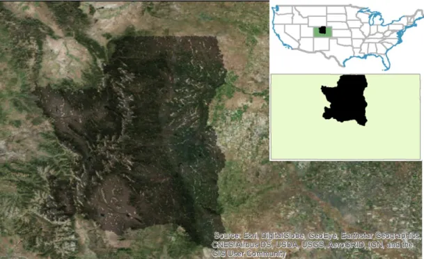
Since one of the goals of this study is to investigate the role of soil moisture assimilation targeting operational flood forecasting systems, modeling floods is of interest. In particular, The great Colorado flood of September 2013 is studied. This flood happened during the period of 9-16 September 2013 due to heavy rainfall (>450 mm) in the Colorado Front Range foothills. The flood caused $2 billion in damage, 8 flood-related fatalities and forced 18,000 people to evacuate their houses (Gochis et al., 2015). Record atmospheric moisture was brought to the region by large-scale moisture advection features and led to heavy rainfall. While numerical weather predictions were able to identify this rainfall, they had significant errors in its magnitude and spatial pattern (Gochis et al., 2015). For a detailed assessment of the causes and impacts of this flood, interested readers are referred to Uccellini (2014). Figure 2-1 shows the location and imagery of this area.
13
Figure 2-1: Imagery and location of the studied area, Colorado Front Range
2.4.2 Satellite soil moisture observations
Frequently used satellite soil moisture products are the Climate Change Initiative (CCI), Soil Moisture and Ocean Salinity (SMOS), Advanced Scatterometer (ASCAT) by European Space Agency (ESA), and Soil Moisture Active Passive (SMAP) by National Aeronautics and Space Administration (NASA).
Available from March 31, 2015, SMAP (Entekhabi et al., 2010) monitors the Earth’s land surface for soil moisture. A unique feature of this mission is its ability to distinguish frozen and thawed land surfaces. SMAP provides more than 20 data products
14
with different spatiotemporal resolutions under four levels of L1, L2, L3, and L4, representing the processing levels. The L1 and L2 products contain instrument-related data based on half orbits of the SMAP satellite. The L3 products are a daily composite of L2. The L4 data are the output from NASA’s land surface model estimated by assimilation of L-band brightness temperature observations. While SMAP measurements provide soil moisture in the upper 5 cm of the soil column, L4 products are designed to provide root zone soil moisture by informing model simulations of surface soil moisture within data assimilation processes. One application that can directly benefit from remotely sensed soil moisture measurements is flood forecasting (Entekhabi et al., 2010) since soil moisture plays an essential role in partitioning rainfall into infiltration and runoff. Accurate observations of current soil moisture status lead to improved flood forecasts. This study investigates the advantages of updated soil moisture states.
Since SMAP data were not available for the 2013 flood, the Climate Change Initiative (CCI) v02.2 (Dorigo et al., 2017; Liu et al., 2011) is used for this case study. Four passive and two active microwaves are blended to form the CCI products including the Scanning Multichannel Microwave Radiometer (SMMR), Special Sensor Microwave Imager (SSM/I), Tropical Rainfall Measure Mission (TRMM) Microwave Imager (TMI), Advanced Microwave Scanning Radiometer for Earth Observing System (AMSR-E), Advanced Microwave Instrument (AMI), and ASCAT. The temporal resolution of CCI data is daily and the spatial resolution is 0.25˚.
15
2.4.3 Meteorological forcing
Two datasets that could potentially be used for Noah-MP are GLDAS (Global Land Data Assimilation System) and NLDAS (North American Land Data Assimilation System). The Global Land Data Assimilation System (GLDAS) (Rodell et al., 2004), built upon the North American Land Data Assimilation System (NLDAS), provides support for improved forecast initial conditions by integrating data from advanced observing systems. GLDAS is a multi-institutional product developed jointly by National Aeronautics and Space Administration (NASA), Goddard Space Flight Center (GSFC), and the National Oceanic and Atmospheric Administration National Centers for Environmental Prediction (NOAA NCEP) and is run at NCEP, NASA GSFC, Princeton University, the University of Washington, and NOAA’s Office of Hydrologic Development. GLDAS drives Mosaic, Noah, CLM, and VIC land surface models with the goal of simulating the transfer of mass, energy, and momentum. Then, it updates the simulations by merging them with satellite- and ground-based observations through data assimilation techniques such as the Ensemble Kalman Filter and the Extended Kalman Filter. GLDAS runs are performed on 0.25˚ × 0.25˚ (standard operational run), 0.5˚×0.5˚, 1.0˚×1.0˚, and 2.0˚×2.5˚ grids and the results are publicly available in near-real time.
Multiple versions of GLDAS are available including GLDAS-2, which refers to simulations forced entirely with Princeton meteorological forcing data, GLDAS-2.1 referring to simulations forced with a combination of model- and observation-based data, and GLDAS-1 which includes simulations forced by combination of NOAA/GLDAS
16
atmospheric analysis fields, spatially and temporally disaggregated NOAA Climate Prediction Center Merged Analysis of Precipitation (CMAP) fields2.
Land surface models, in particular, Noah-MP (Niu et al., 2011; Yang et al., 2011), can be forced with the GLDAS meteorological data such as precipitation, short- (and long-) wave radiation, air temperature, air pressure, specific humidity, and wind speed. For example, Yang et al. (2011) run Noah-MP at a global scale with meteorological forcing data from GLDAS for the period of 1980-2006 in order to assess the performance of Noah-MP.
In this study, the Noah-MP model is forced with surface meteorological data including daily or sub-daily precipitation, wind speed, air temperature, specific humidity, air pressure, and incoming longwave and shortwave radiation. Meteorological forcings were obtained from the Phase II North American Land Data Assimilation System (NLDAS-2) (Xia et al., 2012b), gridded to the 1/8˚ resolution. NLDAS is a multi-institution project aiming at providing reliable initial land states to improve weather predictions. NLDAS runs Noah, Mosaic, Sacramento Soil Moisture Accounting (SAC-SMA), and VIC to generate land states over 1/8˚ CONUS domain (Xia et al., 2012a). NLDAS-1 was first introduced by Mitchell et al. (2004) and later in 2012 NLDAS-2 which builds on NLDAS-1 was published. The second phase increased the accuracy and consistency of the data and upgraded the model codes and parameters.
2
For more information, visit
17
2.5 Noah-MP Land Surface Model
A Land Surface Model (LSM) is a mathematical representation of a hydrologic system that simulates energy and water fluxes. LSMs are categorized into two categories of lumped and distributed. While lumped models simulate the entire basin as one entity with forcing data (input) uniformly distributed across the basin, distributed models divide the watershed into smaller units (e.g., grid cells) and solve the energy and water balance for each unit. Some well-known distributed models include (but are not limited to) Variable Infiltration Capacity (VIC) (Liang et al., 1994; Nijssen et al., 2001), Community Land Model (CLM) (Oleson Lawrence, D. M., Bonan, G. B., Flanner, M. G., et al., 2010), Noah (Ek, 2003), and Noah-MP (Yang et al., 2011).
Noah LSM is a result of multi-institutional cooperation including the Air Force Weather Agency, Weather Research and Forecast (WRF), and the National Center for Environmental Prediction (NCEP). The model is reported to have shortcomings on the following processes:
1) Runoff and snowmelt simulations (Bowling et al., 2003; Slater et al., 2007).
2) Snow skin temperature prediction as a result of combining vegetation and snow layers in snowy days (Niu et al., 2011).
3) Capturing the Earth’s critical zone because the model considers just a shallow soil column (only two meters) which then results in a relatively short soil memory (Niu et al., 2011).
18
4) Representing infiltration in the presence of frozen soil (Shanley and Chalmers, 1999).
However, Noah-MP (Yang et al., 2011) attempts to resolve the above weaknesses by adding a vegetation canopy layer, modifying the radiation transfer system, and relating stomatal resilience to photosynthesis. In addition to solving the aforementioned problems (Barlage et al., 2015), Noah-MP offers alternatives for various physical processes. For instance, multiple options are provided for dynamic vegetation, frozen soil permeability, conversion of precipitation into rainfall/snowfall, generation of runoff/groundwater, and more processes as discussed in Niu et al. (2011). A performance assessment of Noah-MP (Yang et al., 2011) concluded that despite the amplified computational time, the model demonstrates improvements in skin temperature, runoff, snow, and soil moisture simulations as compared to the original Noah LSM. Furthermore, the optional parameterization schemas of the Noah-MP model was proven beneficial after conducting 36 experiments with 36 different combinations of parameter schemas concluding that the ensemble mean performs better than any individual ensemble member (Yang et al., 2011).
Noah-MP has attracted attention from the meteorological and hydrological communities. The meteorological community is interested in this model mainly because it has been coupled with the Weather Research and Forecast (WRF) model. Such coupling enables the modeling of the land-atmosphere feedbacks. Coupled Noah LSM has been used in operational agencies such as the National Center for Environmental
19
Prediction (NCEP) for weather prediction and downscaling of the climate models (Yang et al., 2011); Noah-MP is a possible replacement. Additionally, Noah-MP was tested for inclusion in the next phase of the North American Land Data Assimilation System (NLDAS) (Cai et al., 2014b). On the other hand, the hydrologic community has become interested in this model because it is the main LSM in the National Water Model (NWM) operated by the National Weather Service (NWS) for flood forecasting in more than 2 million river reaches over the Continental United States.
A brief literature review on the Noah-MP model is presented in the following. More specific information such as setting up the model is discussed in the “results” section.
Model background: Noah-MP is developed in FORTRAN and is forced with the air temperature at height z above ground, snowfall, rainfall, surface downward solar radiation, surface downward longwave radiation, specific humidity at height z above ground, and surface pressure at height z above ground. It is noteworthy that the entire forcing variables are available through the Global Land Data Assimilation System (GLDAS) (Rodell et al., 2004).
Xia et al. (2017) discussed the next generation of NLDAS using three LSMs including Noah-MP, Community Land Model version 4.0 (CLM4.0), and Catchment LSM-Fortuna 2.5 (CLSM-F2.5). They concluded that all three models were able to capture monthly to inter-annual variability. They also discussed that current LSMs in
20
NLDAS have a simple snow model, which causes an unrealistic runoff simulation and thus, Noah-MP can be of interest.
Model sensitivity: Cuntz et al. (2016) performed a global sensitivity analysis of Noah-MP parameters. In addition to 71 model parameters, they found 139 hard-coded parameters and included them in their analysis and found that the most sensitive parameter is a hard-coded one that controls soil surface against direct evaporation. They find that latent heat3 and runoff have similar sensitivities and that surface runoff is sensitive to almost all of the hard-coded parameters. They also argue that the model is sensitive to the quality of incoming radiation. They suggested that the user should take care of the amount of direct diffusive radiation and the amount of visible to near-infrared radiation in the input files.
Arsenault et al. (2018) conducted a sensitivity analysis of Noah-MP. They used a variance decomposition method to assess model sensitivity to its parameters. Their target variables were soil moisture, sensible heat, latent heat, and net ecosystem exchange. They have done the analysis on 10 international Fluxnet stations over the globe. They considered four configurations and concluded that in dynamic vegetation configuration, all output variables were very sensitive to wilting point, unsaturated soil conductivity exponent, baseline light use efficiency, baseline carboxylation, leaf turnover, and single-sided leaf area. Particularly for soil moisture, they considered porosity and saturated soil
3 The hidden (latent=hidden) heat absorbed or released in processes that the temperature remains
21
hydraulic conductivity. They also conclude that dynamic vegetation configuration makes soil moisture more sensitive to vegetation parameters. This highlights the potential of using a land surface model with dynamic vegetation option to improve soil moisture state estimates (Yang et al., 2011).
Model performance: Model performance of Noah-MP was first evaluated by Yang et al. (2011) where global-scale tests were conducted on the model. By comparing model simulations against satellite and ground-based observations, they showed improvements in modeling runoff, soil moisture, snow, and skin temperature as compared to the Noah LSM. They design six experiments ranging from Noah LSM to fully augmented Noah-MP with dynamic vegetation. They also made an ensemble of different schemas and recommended that the model should be used in an ensemble format. An important note regarding the Noah-MP LSM is that the mean state and variability of the model are controlled by ET but modulated by the buffering effects due to groundwater (Yang et al., 2011). Yang et al. (2011)discuss that the runoff schema plays a vital role in soil moisture-ET relationship. Four options are provided for calculating runoff. These options include Simple Top Runoff and Groundwater Model (SIMGM), Simple Top Runoff Model (SIMTOP), and Schaake96. SIMGM refers to TOPMODEL-based runoff scheme with the simple groundwater (Niu et al., 2011), SIMTOP refers to a simple TOPMODEL‐based runoff scheme with an equilibrium water table (Niu et al., 2011), and Schaake96 refers to an infiltration‐excess‐based surface runoff scheme. This scheme uses a gravitational free‐drainage subsurface runoff process which was used in the original
22
Noah model as well (Schaake et al., 1996). The last runoff schema option is BATS. Surface runoff in BATS is parameterized as a 4th power function of the top 2 m soil wetness. The subsurface runoff is parameterized as gravitational free drainage (Niu et al., 2011). Yang et al. (2011) discuss that some schemas such as SIMTOP result in the wetter soil as they impose a lower boundary condition (zero-flux). Runoff schemas with gravitational free drainage (such as BATS) tend to underestimate soil moisture, which in turn leads to underestimation of ET as compared to models with a groundwater component. While the runoff schema is a key schema for soil moisture modeling, as concluded by Yang et al. (2011), the β factor (a factor in Noah-MP that controls stomatal resistance), dynamic vegetation, and stomatal resistance are not as important.
The 2m maximum temperature is very sensitive to the choice of the LSM as Burakowski et al. (2016) showed. Zhang et al., (2016) showed that these subprocess schemas have the highest uncertainty: canopy resistance, soil moisture threshold for evaporation, runoff and groundwater, and surface-layer parameterization. Ma et al. (2017) evaluate Noah-MP’s performance over 18 HUC2 regions across the CONUS. They observed that the model performs better in simulating evapotranspiration when the dynamic vegetation option is off and they conclude that the dynamic vegetation option needs to be improved. Ma et al. (2017),Niu et al. (2011), and Yang et al. (2011) confirmed that Noah-MP performs well in simulating snow depth and snow water equivalent (SWE).
23
Martinez et al. (2016) concluded that an increase in root-zone soil moisture (top 2 meters) results in an increase of evapotranspiration, mostly in areas where ET is more water limited. They also found that the groundwater schemas induce an increase in the simulated moisture where the water table is close to the surface. They discussed that when the increase in ET takes place in areas that water table is in the root-zone, part of the extra ET comes from direct uptake of moisture from the saturated layers below the water table (i.e., direct groundwater uptake).
Model spin-up: Cai et al. (2014a) analyzed the required spin-up duration for soil moisture and suggested that 8 years is enough for the analysis. Gao et al. (2015) discussed the spin-up period for the Noah-MP model and highlighted the importance of spin-up in Noah-MP. The required spin-up period may vary from a couple of years to more than 30 years, depending on the variable of interest and the physics of the model. For example, Gao et al., (2015) discussed that for a simple soil physics, 4 years of spin-up would be enough, while in case of adding organic matter and spare to dense rhizosphere parameterization, 30 years of spin-up is needed.
Coupling with climate models: Gao et al. (2015) discussed that the interactions between land and atmosphere are not well represented in the current LSMs. Therefore, they used Noah-MP to assess the parameterization role in Tibetan Plateau (TP). They concluded that uncertainty in soil initialization significantly affects deep-soil temperature and moisture. They discussed that the uncertainties in atmospheric forcings affects topsoil variables, and therefore the surface energy fluxes. They showed that the default Noah-MP
24
has large dry biases (about 50%) in topsoil moisture in the monsoon season. They reported successful results when the rhizosphere effect is taken into consideration.
2.6 Methodology
2.6.1 Data Assimilation
In this study, both EnKF and PF-MCMC are used and their performance in improving soil moisture simulations is assessed. In the following section, a brief literature review on both methods is presented.
2.6.1.1Particle Filter
Particle Filter (PF) methods have been frequently demonstrated to be effective in hydrologic modeling (Dechant and Moradkhani, 2011; Moradkhani et al., 2018, 2012; Yan and Moradkhani, 2016). Similar to all PFs, PF-MCMC is also based on Sequential Importance Resampling (SIS) (Liu et al., 2001). Due to weight degeneracy as a shortcoming of SIS, a resampling step is introduced where particles with significant weights are replicated and particles with insignificant weights are neglected (Moradkhani et al., 2012). Markov Chain Monte Carlo (MCMC) methods are introduced as an alternative of PFs that are based on the Ergodic theory4 while PFs are based on the law of large numbers (Moradkhani et al., 2012). These techniques explore the posterior distribution using one or more chains and are more efficient than the PF methods (Moradkhani et al., 2012). MCMC methods are one of the ten most influential algorithms
4
25
of the 20th century (Dongarra and Sullivan, 2000). In simple words, the goal of MCMC is to sample from a complicated, high-dimensional function. However, the function is too complicated to sample from. One way to tackle this problem is importance sampling where there is a proposal distribution to sample from. This proposal distribution could successfully mimic the original posterior distribution in low dimensions; however, for higher dimensions, the proposal distribution can incorrectly assign higher probabilities. Therefore, the proposal distribution could fail in high dimensions. MCMC methods propose to tackle this problem by a random walk in the areas with high probabilities.
The particle filter (PF) based ensemble DA algorithm is used in this study to update the model states and quantify the initial condition uncertainty. Compared with the popular ensemble Kalman filter (EnKF), the PF can relax the Gaussian error assumption, maintain water balance, and provide a more complete representation of state/parameter posterior distribution (Dechant and Moradkhani, 2014; Moradkhani et al., 2012; Yan and Moradkhani, 2016; Yan et al., 2015).
As demonstrated by Moradkhani (2008), the state-space models that describe the generic earth system are as follows:
( ) (1)
( ) (2)
where is a vector of the uncertain state variables at a current time step, is a vector of observation data, is the uncertain forcing data, is the
26
model parameters, h is a non-linear function that relates the states to the observations , represents the model error, and indicates the observation error. The errors and are assumed to be white noise with mean zero and covariance and , respectively. The posterior distribution of the state variables given a realization of the observations is written as follows:
( ) ( ) ( ) ( ) ( ) ( ) ( ) ∫ ( ) ( ) (3) ( ) ∫ ( ) ∫ ( ) ( ) (4)
where ( ) is the likelihood, ( ) is the prior distribution, and ( ) is the normalization factor. In practice, Equation (3) does not have an analytic solution except for a few special cases. Instead, the posterior distribution
( ) is usually approximated using a set of Monte Carlo (MC) random samples as:
( ) ∑ ( )
(5)
where is the posterior weight of the particle, is the Dirac delta function, and is the ensemble size. The normalized weights are calculated as follows:
27
( )
∑ ( )
(6)
where is the prior particle weights, and ( ) can be computed from the likelihood ( ). Generally, a Gaussian distribution is used to estimate ( ):
( )
√( ) [ ( ( ))
( ( ))]
(7)
To obtain approximate samples from ( ), a resampling operation is necessary. Moradkhani et al. (2005a) suggest resampling the particles with a probability greater than the uniform probability. After resampling, all the particle weights are set equal to ⁄ .
To further reduce the weight degeneration problem (where all but one of the importance weights are close to zero), the particle filter with sampling importance resampling (PF-SIR) algorithm can be combined with Markov chain Monte Carlo (MCMC) (Andrieu et al., 2010; Moradkhani et al., 2012). The recently developed particle Markov chain Monte Carlo (PMCMC) (Andrieu et al., 2010) is used in this study for large-scale DA applications. The PMCMC is an extension of the SIR and uses the PF-SIR to design efficient high-dimensional proposal distributions for the MCMC algorithm.
The PMCMC consists of the following three steps: (1) Initialization ( ): run PF-SIR targeting ( ), sample ( ) ( ) and let ( )( ) denote the corresponding marginal likelihood estimate. (2) Iteration ( ): sample ( )