Object Retrieval with Deep Convolutional
Features
Eva Mohedanoa, Amaia Salvadorb, Kevin McGuinnessa, Xavier Gir´o-i-Nietob, Noel E. O’Connoraand Ferran Marqu´esb
aInsight Center for Data Analytics, Dublin City University bImage Processing Group, Universitat Polit`ecnica de Catalunya
Abstract. Image representations extracted from convolutional neural networks (CNNs) outdo hand-crafted features in several computer vision tasks, such as visual image retrieval. This chapter recommends a simple pipeline for encoding the local activations of a convolutional layer of a pre-trained CNN utilizing the well-known Bag of Words (BoW) aggregation scheme and called bag of local convolutional features (BLCF). Matching each local array of activations in a convolutional layer to a visual word results in anassignment map, which is a compact representation relating regions of an image with a visual word. We use the assignment map for fast spatial reranking, finding object localizations that are used for query expansion. We show the suitability of the BoW representation based on local CNN features for image retrieval, attaining state-of-the-art performance on the Oxford and Paris buildings benchmarks. We demonstrate that the BLCF system outperforms the latest procedures using sum pooling for a subgroup of the challenging TRECVid INS benchmark according to the mean Average Precision (mAP) metric.
Keywords. Information Storage and Retrieval, Content Analysis and Indexing, Image Processing and Computer Vision, Feature Representation, Convolutional Neural Networks, Deep Learning, Bag of Words
1. Introduction
Visual image retrieval aims at organizing and structuring image databases based on their visual content. The proliferation of ubiquitous cameras in the last decade has motivated researchers in the field to push the limits of visual search systems with scalable yet effective solutions.
Representations based on convolutional neural networks (CNNs) have been demonstrated to outperform the state-of-the-art in many computer vision tasks. CNNs trained on large amounts of labeled data produce global representations that effectively capture the semantics in images. Features from these networks have been successfully used in various image retrieval benchmarks with very promising results [1,2,3,4,5,6], improving upon the state-of-the-art compact image representations for image retrieval.
Despite CNN-based descriptors performing remarkably well in instance search benchmarks like the Oxford and Paris Buildings datasets, state-of-the-art
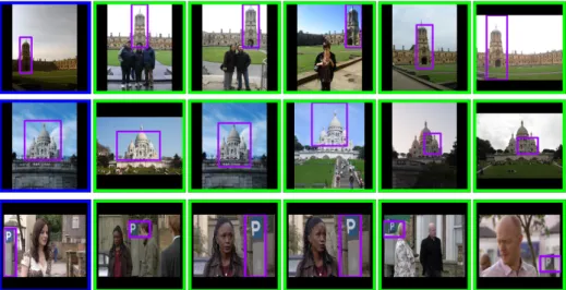
an-Figure 1. Examples of the top-ranked images and localizations based on local CNN features encoded with BoW. Top row: The Christ Church from the Oxford Buildings dataset; middle row: The Sacre Coeur from Paris Buildings; bottom row: query 9098 (a parking sign) from TRECVid INS 2013.
swers for more challenging datasets such as TRECVid Instance Search (INS) have not yet adopted pipelines that depend solely on CNN features. Many INS systems [7,8,9,10] are still based on aggregating local handcrafted features (like SIFT) using the Bag of Words encoding [11] to produce very high-dimensional sparse image representations. Such high-dimensional sparse representations have several benefits over their dense counterparts. High dimensionality means they are more probable to be linearly separable while presenting relatively few non-zero elements, which makes them efficient equally in terms of storage (only nonzero components need to be stored), and computation (only non-zero elements need to be visited). Sparse representations can handle varying information content and are less likely to interfere with one another when pooled. From an information retrieval perspective, sparse representations can be stored in inverted indices, which facilitates efficient selection of images that share features with a query. Furthermore, there is considerable evidence that biological systems make extensive use of sparse representations for sensory information [12,13]. Empirically, sparse representations have repeatedly demonstrated to be effective in a wide range of vision and machine learning tasks.
Many efficient image retrieval engines combine an initial highly scalable ranking mechanism on the full image database with a more computationally expensive yet higher-precision reranking scheme applied to the top retrieved items. This reranking mechanism often takes the form of geometric verification and spatial analysis [14,15,16,8], after which the best matching results can be used for query expansion (pseudo-relevance feedback) [17,18].
In this chapter, inspired by advances in CNN-based descriptors for image retrieval, yet still focusing on instance search, we revisit the Bag of Words encoding scheme using local features from convolutional layers of a CNN. This work presents the following contributions:
• We conduct a comprehensive state-of-the-art review analyzing contemporary approaches using CNN models for the task of image retrieval.
• We propose a sparse visual descriptor based on a bag of local convolutional features (BLCF), which permits fast image retrieval via an inverted index.
• We present the assignment map as a novel compact representation of the image, which maps image pixels ito their corresponding visual words. The assignment map allows fast creation of a BoW descriptor for any region of the image.
• We take advantage of the scalability properties of the assignment map to achieve a local analysis of multiple regions of the image for reranking, followed by a query expansion stage using the obtained object localizations. Using this approach, we present an image retrieval system that achieves state-of-the-art performance comparing with other non-fine tuned models in content-based image retrieval (CBIR) benchmarks and outperforms current state-of-the-art CNN based descriptors at the task of instance search. Figure 1 illustrates some of the rankings produced by our system on three different datasets.
The remainder of the chapter is structured as follows. Section 2 contains an extensive overview of related work. Section3 presents different retrieval benchmarks. Section 4 introduces the proposed framework for BoW encoding of CNN local features. Section 5 explains the details of our retrieval system, including the local reranking and query expansion stages. Section 6 presents experimental results on three image retrieval benchmarks (Oxford Buildings, Paris Buildings, and a subset of TRECVid INS 2013), as well as a comparison to five other state-of-the-art approaches. Section 7 summarizes the most significant results and outlines future work.
2. Related Work
2.1. First CNN Approaches for Retrieval
Several other authors have proposed CNN-based representations for image retrieval. The first applications focused on replacing traditionally handcrafted descriptors with features from a pre-trained CNN for image classification. Activations from the last fully connected layers from the Alexnet network proposed by Krizhevsky were the first ones to be used as a generic image representation with potential applications for image retrieval [19,20,21]. Similar images generate similar ac-tivation vectors in the Euclidean space. This finding motivated early works in studying the capability of CNN models for retrieval, mostly focused on the analysis of fully connected layers extracted from pre-trained CNN classification model Alexnet [2,3,22]. In this context, Babenko et al. [2] showed how such features could reach similar performance to handcrafted features encoded with Fisher vectors for image retrieval. Razavian et al. [3] later outperformed the state-of-the-art of CNN representations for retrieval using several image sub-patches as input to a pre-trained CNN to extract features at different locations of the image. Similarly, Liu et al. [23] used features from fully connected layers evaluated on image sub patches to encode images using Bag of Words.
2.2. Convolutional Features for Retrieval
While descriptors from fully connected layers of a pre-trained CNN in ImageNet achieve competitive performance, local characteristics of objects at instance level are not well preserved at those layers, since information contained is biased towards the final classification task (too semantic) and spatial information is completely lost (each neuron in a fully connected layer is connected to all neurons of the previous layer).
A second generation of works reported significant gains in performance when switching from fully connected to convolutional layers. Razavian et al. [4] performed spatial max pooling on the feature maps of a convolutional layer of a pre-trained CNN to produce a descriptor of the same dimension as the number of filters of the layer. Babenko and Lempitsky [1] proposed sum-pooled convolutional features (SPoc), a compact descriptor based on sum pooling of convolutional feature maps preprocessed with a Gaussian center prior. Tolias et al. [5] introduced a feature representation based on the integral image to quickly max pool features from local patches of the image and encode them in a compact representation. The work by Kalantidis et al. [24] proposed Cross-dimensional weighting and pooling(CroW), a non-parametric spatial and channel-wise weighting schemes applied directly to the convolutional features before sum pooling. Our work shares similarities with all the former in that we use convolutional features extracted from a pre-trained CNN. Unlike these approaches, however, we propose a sparse, high-dimensional encoding that better represents local image features, particularly in difficult instance search scenarios where the target object is not the primary focus of the image.
Several authors have tried to exploit local information in images by passing multiple image sub patches through a CNN to obtain local features from either fully connected [3,23] or convolutional [22] layers, which are in turn aggregated using techniques like average pooling [3], BoW [23], or Vector of Locally Aggregated Descriptors (VLAD) [22]. Although many of these methods perform well in retrieval benchmarks, they are significantly more computationally costly since they require CNN feature extraction from many image patches, which slows down indexing and feature extraction at retrieval time.
An alternative approach is to extract convolutional features for the full image and treat the activations of the different neuron arrays across all feature maps as local features. This way, a single forward pass of the entire image through the CNN is enough to obtain the activations of its local patches. Following this approach, Ng et al. [25] proposed to use VLAD [26] encoding of features from convolutional layers to produce a single image descriptor. Arandjelovi´c et al. [27] chose to adapt a CNN with a layer especially trained to learn the VLAD parameters. Our approach is similar to the ones in [25,27] in that we also treat the features in a convolutional layer as local features extracted at different locations in an image. We, however, use BoW encoding instead of VLAD to take advantage of sparse representations for fast retrieval in large-scale databases.
Several of the cited approaches propose systems that are based or partially based on a spatial search over multiple regions of the image. Razavian et al. [4] achieve a remarkable increase in performance by applying a spatial search strategy over an arbitrary grid of windows at different scales. Although they report high
accuracy in several retrieval benchmarks, their proposed approach is very compu-tationally costly and does not scale well to larger datasets and real-time search scenarios. Tolias et al. [5] introduce a local analysis of multiple image patches, which is only applied to the top elements of an initial ranking. They propose an efficient workaround for sub patch feature pooling based on integral images, which allows them to quickly evaluate many image windows. Their approach improves their baseline ranking and provides approximate object localizations. They apply query expansion using images from the top of the ranking after the reranking stage, although they do not use the obtained object locations in any way to improve retrieval performance. In this direction, our work proposes using the assignment map to quickly build the BoW representation of any image patch, which allows us to apply a spatial search for reranking. We apply weak spatial verification to each target window using a spatial pyramid matching strategy. Unlike [5], we use the object localizations obtained with spatial search to mask out the activations of the background and perform query expansion using the detected object location.
Another method to improve the representativeness of the convolutional features is weighting them with some sort of attention map. Jimenez et al. [28] have proposed a technique that can be seen as a combination of the ideas introduced in CroW [24] and R-MAC [5]. They propose using Class Activation Maps (CAMs) [29], which is technique that can be applied to most of the the state-of-the-art CNN networks for classification to create a spatial map highlighting the contribution of the areas within an image that are more relevant for the network to classify an image as one particular class. This way, several weighting schemes can be generated for each of the classes for which the original pre-trained network was trained (typically the 1000 classes of ImageNet [30]). Each of the weighting schemes can be used in the same way as in CroW to generate different vectors per class. All the obtained class-vectors are then sum-pooled to get a final compact representation. BLCFs can also be enriched with a weighting scheme, as proposed in [31]. In this case, instead of weighting them with a class-activation map, the attention map was computed with a prediction of the gaze fixation over egocentric images. In this, case, a visual saliency map was estimated with SalNet [32], a deep convolutional network trained for that purpose.
Focused on exploring the advantage of processing different regions of the image independently, Salvadoret al.[33] propose to use a fine-tuned version of an object detection network. In particular, they use the Faster R-CNN [34] which is a network composed of a base module, which is a fully convolutional CNN (i.e VGG16 architecture), and a top module composed of two branches: one branch is a Region Proposal Network that learns a set of window locations, and the second one is a classifier (composed by three fully connected layers) that learns to label each window as one of the classes in the training set. Object proposals can be understood as a way of focusing in specific areas of the image so they are equivalent to a weighting scheme if their features are pooled. In this sense, BLCF may also benefit some these type of tools at the expense of an additional computation time and indexing resources.
2.3. End-to-End Learning
Deep learning has been proven as a mechanism to successfully learn useful semantic representations from data. However, most of the discussed work use off-the-shelf CNN representations for the task of retrieval, where representations have been implicitly learned as part of a classification task on ImageNet dataset. This approach presents two main drawbacks: the first one comes from thesource dataset
ImageNet from where features have been learned. While Imagenet is a large-scale dataset for classification, covering diverse 1000 classes (from airplanes, landmarks, general objects) and allowing models to learn good generic features, it has been explicitly designed to contain high intra-class invariance which is not a desirable property to retrieval. The second, consists in the usedloss function: Categorical cross entropy evaluates the classification prediction without trying to discriminate between instances from the same class, which may be desirable in several retrieval scenarios.
One simple but yet effective solution to improve the capacity of the CNN features consists in learning representations that are more suitable to the test retrieval dataset by fine-tuning the CNN network to perform classification in a new domain. This approach was followed by Babenko [2], where the Alexnet architecture was trained to perform classification in a Landmark1 dataset, more semantically similar to the target retrieval domain. Despite improving performance, the final metric and the layers utilized were different to the ones actually optimized during learning.
State-of-the art CNN retrieval networks have been tuned optimizing a similarity loss function [35,4,26]. For that, the whole fine-tuning process of a CNN is casted as a metric learning problem, where the CNN represents an embedding function that maps the input image into a space where relative image similarities are preserved.Siamese andTriplet networks are commonly used for that task.
2.3.1. Siamese Networks
Siamese networks [36,37,38] are architectures composed by two branches (composed by convolutional, ReLu, Maxpooling layers) that share exactly the same weights across each layer. It is trained on paired data consisting in an image pair (i, j) whereY(i, j)∈ {0,1} represents the binary label indicating if the images belong to the same category or not. The network optimizes the contrastive loss function defined for each pair as
L(i, j) =1
2(Y(i, j)D(i, j) + (1−Y(i, j)) max(0, α−D(i, j))), (1) where D(i, j) represents the Euclidean Distance between a pair of images D(i, j) =kf(i)−f(j)k2 andfthe embedding function (CNN network) that maps an image to a point in an Euclidean space. When a pair of images belong to the same category, the loss function tries to directly reduce the distance in the feature space, whereas when images are different the loss is composed by a hinge
function that maximizes those distances, which are too small as they do not reach a minimum marginα.
First introduced in 1994 for signature verification [39], Siamese networks have been applied for dimensionality reduction [37], learning image descriptors [40,41,42] or face verification [36,38].
2.3.2. Triplet Networks
Triplet networks are an extension of the Siamese networks where the loss function minimizes relative similarities. Each training triplet is composed by an anchor
or reference image, a positive example of the same class as the anchor, and a negative example of a different class to the anchor. The loss function is defined by the hinge loss as
L(a, p, n) = max(0, D(a, p)−D(a, n) +α), (2)
where D(a, p) is the Euclidean distance between the anchor and a positive example, D(a, n) is the Euclidean distance between the anchor and a negative example andαa margin. The loss ensures that given an anchor image, the distance between the anchor and a negative image is larger than the distance between the anchor and a positive image by a certain margin α.
The main difference between triplet and Siamese architectures is that the former one optimizes relative distances with a reference image or anchor, whereas the later optimizes separately positive and negative pairs; which usually leads to models with better performance [43,44].
2.3.3. Training Data for Similarity Learning
Generating training data for similarity learning is not a trivial task. A usual procedure of collecting a new image dataset is mainly divided into two steps:
• Web crawling: Given pre-defined text queries depicting different categories,
querying them in some of the popular image search engines (Google Image Search, Bing, Flick) to download a set of noisy labeled images.
• Data cleaning: Images retrieved by available search engines usually contain
noisy results such as near-duplicates or unrelated images, high intraclass image variations such interior or exterior images of a particular building or high diversity in the image resolution. Two approaches are followed after the web crawling:
∗ Manual data cleaning: Which can be based on manual processing, ex-haustively inspecting all images for a dataset of moderate or small sizes [1,45,46,?] or by making use of a crowdsourcing mechanism such as Amazon Mechanical Turk for large scale datasets [30,47,48].
∗ Automatic data cleaning: In this approach, metadata associated with the images is exploited as an additional filtering step such as geo-tagged datasets [49,27] and/or the usage of image representations to estimate similarity and geometry consistence between images, a process that usually rely in handcrafted invariant features [50,35,51].
2.3.4. Hard Negative Mining
During learning, networks are optimized via mini-batch Stochastic Gradient Descent (SGD). Sampling pairs or triplets at random is an inefficient strategy because many of them can already accomplish the margin criteria of equations 1 and 2. That means that no error is generated and no gradients are backpropagated, so the weights of the CNN model are not updated and no learning is performed. To sample positive pairs, a common procedure consists of sampling images that belong to the same class [35], 3D point or cluster [41,51]. Some approaches select positive pairs with minimal distance within the initial embedding space [26]. In order to avoid sampling very similar images, Radenovi´cet al [51] make use of the strong matching pipeline with 3D reconstruction to select only positives that share the minimum amount of local matches, so matching images depict the same object but also ensuring variability of viewpoints.
For the negative pairs, a common procedure consists in iterating over non-matching images that are “hard” negatives, those being close in the descriptor space and that incur a high loss. For that, the loss is computed over a set of negative pairs and only a subset with higher losses is selected for training. This procedure is repeated every N iterations of SGD, so hard examples are picked during all the network learning [41,35]. Variability in the sampling is ensured in [51] by selecting the negative pairs from different clusters or 3D points. Selecting negative pairs based on the loss generally leads to multiple and very similar instances of the same object.
More sophisticated approaches take advantage of the training batches. For instance, Songet al.[52] propose a loss function that integrates all positive and negative samples to form a lifted structured embedding. A smart mining represents crucial step for succeeding in training SML models and is an active research area.
2.4. Retrieval CNN Architectures
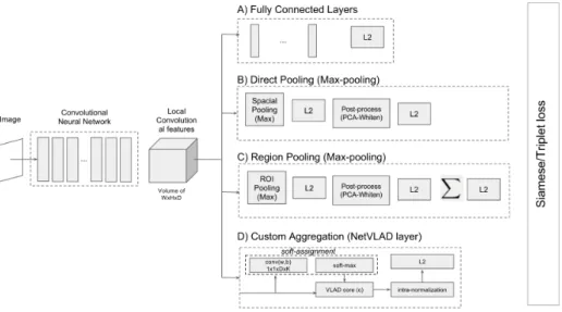
Recent end-to-end networks proposed for retrieval are based on state-of-the-art architectures for image classification (Alexnet, VGG16, ResNet50). Final retrieval representations are built from convolutional layers. Architectures mainly differ in the top layers designed to aggregate the local convolutional features, as illustrated in Figure 2.
Some of the approaches directly fine-tune the original classification network [48, 50,53], using fully connected layers as image representations. For instance, the full Alexnet architecture is used in [48], where authors explore a multitask learning by optimizing the model for similarity learning along with a classification loss for product identification and search. To switch between classification and similarity comparison, the “softmax” operation at the end of the network is replaced with an inner product layer with aL2-normalized vector. The full architecture Alexnet is also used in [50], in this case, two additional channels containing a shallow CNN are considered to process two low-resolution versions of the original image. With that, the final descriptor includes multi-scale information to alleviate the limitations of working with fully connected layers. Similarly, Wan et al [53] perform the fine-tuning of Alexnet directly on the Oxford and Paris datasets. The three approaches, however, heavily rely on manually annotated data [53,48] or
Figure 2. Architectures for similarity learning. The baseline network is initialized with the weights of a state-of-the-art CNN for classification. The top layer can be seen as the aggregation step base in: A) fully connected layers [53]. Approaches dominated by direct pooling: B) direct pooling sum/max-pooling followed by feature post processing [51] and C) Region pooling followed by feature post processing [35] and D) custom aggregation model such as VLAD [27].
a combination of human annotations with a relevance score for image based in handcrafted descriptors [50].
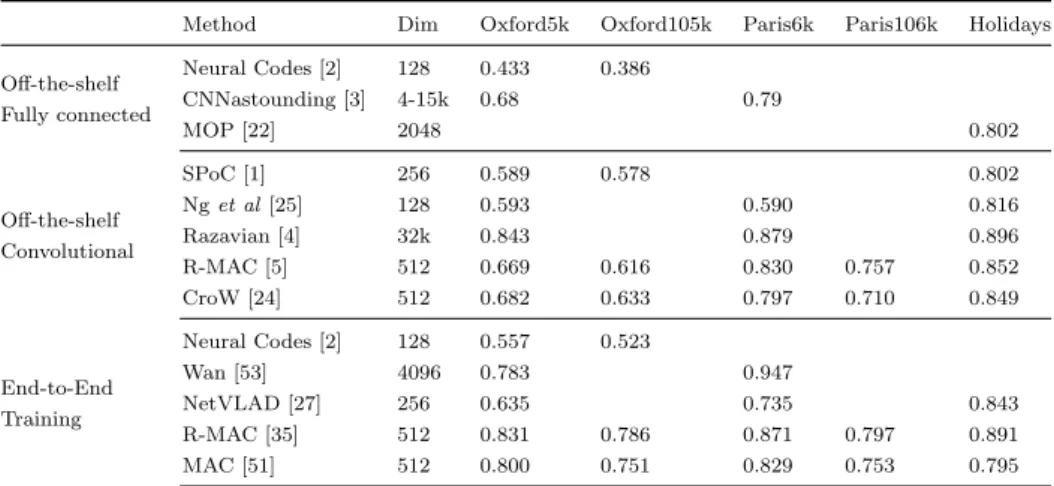
Recent works based their architectures in VGG16 exploiting the capabilities of convolutional layers [51,35,27]. Gordoet al et al [35] proposed a fine-tuned version of Regional Maximum Activation of Convolutions (R-MAC) [5], where a Region Proposal Network (RPN) [34] is learned as a replacement of the fixed grid originally proposed in [5]. PCA is modeled with a shifting and a fully con-nected layer that are tuned during the optimization process for similarity learning. Randenovi´c [51] follows the same architecture as in [35] but directly pooling all descriptors generated by the convolutional layer (MAC), without learning an RPN. PCA transformation is learned via linear discriminant projections proposed by Mikolajczyk and Matas [54] using the annotated training data. Arangjelovi´c [27] propose a more sophisticated encoding by implementing a VLAD layer on top of the convolutional features using soft-assignments to be able to tune the parameters via backpropagation. Similarly, Fisher-Vector layer has been proposed in [55] to aggregate deep convolutional descriptors. Although those approaches follow automatic cleaning process (exploiting the GPS associated to with the images [27] or annotating the images based on strong handcrafted baselines [35,51]), image domain is restricted to landmarks and it is uncertain how models perform in more challenging retrieval scenarios.
Table 1 contains the performance of the discussed CNN approaches. Fine-tuned models for retrieval clearly generate better descriptors than those generated by off-the-shelf networks. However, generating a suitable training dataset for retrieval relies in human annotations and computational expensive annotation
pro-Table 1. Summary discussed CNN approaches in different retrieval benchmarks. The table does not include approaches with spatial verification and re-ranking pipelines.
Method Dim Oxford5k Oxford105k Paris6k Paris106k Holidays Off-the-shelf Fully connected Neural Codes [2] 128 0.433 0.386 CNNastounding [3] 4-15k 0.68 0.79 MOP [22] 2048 0.802 Off-the-shelf Convolutional SPoC [1] 256 0.589 0.578 0.802 Nget al[25] 128 0.593 0.590 0.816 Razavian [4] 32k 0.843 0.879 0.896 R-MAC [5] 512 0.669 0.616 0.830 0.757 0.852 CroW [24] 512 0.682 0.633 0.797 0.710 0.849 End-to-End Training Neural Codes [2] 128 0.557 0.523 Wan [53] 4096 0.783 0.947 NetVLAD [27] 256 0.635 0.735 0.843 R-MAC [35] 512 0.831 0.786 0.871 0.797 0.891 MAC [51] 512 0.800 0.751 0.829 0.753 0.795
cedures that limits the generalization of the methods, usually related to landmarks scenarios.
Despite the rapid advances of CNNs for image retrieval, many state-of-the-art instance search systems are still based on Bag of Words encoding of local handcrafted features such as SIFT [56]. The Bag of Words model has been enhanced with sophisticated technique such as query foreground/background weighting [57], asymmetric distances [58], or larger vocabularies [45,10]. The most substantial improvements, however, are those involving spatial reranking stages. Zhou et al. [9] propose a fast spatial verification technique which benefits from the BoW encoding to choose tentative matching feature pairs between the query and the target image. Zhang et al. [8] introduce an elastic spatial verification step based on triangulated graph model. Nguyen et al. [7] propose a solution based on deformable parts models (DPMs) [59] to rerank a BoW-based baseline. They train a neural network on several query features to learn the weights to fuse the DPM and BoW scores. In our work, we revisit the Bag of Words encoding strategy and demonstrate its suitability to aggregate CNN features of an off-the-shelf network, instead of using handcrafted ones such as SIFT. Our method is unsupervised and does not require of any additional training data, and it is not restricted to any particular domain. We also propose a simple and efficient spatial reranking strategy to allow query expansion with local features. Although we do not use many of the well-known improvements to the BoW pipeline for image search [57,45,58], we propose a baseline system in which they could be easily integrated.
3. Image Retrieval Benchmarks
Publicly available image retrieval benchmarks such as the Oxford Buildings [45], Paris dataset [46], Sculptures [60], INRIA Holidays [61] or Kentucky [62] are relatively small size datasets used in the image retrieval community to test and to compare different approaches for CBIR systems (see Table 2). Results are reported in terms of mean Average Precision (mAP) of the list of images retrieved
from the dataset per query. Metrics such as memory or time required to conduct the search are also important factors to take into account for most real-world problems or when dealing with video, due to the large quantity of images in the dataset. Some recent works reported excellent results using CNNs as image representations [4,35,51,53].
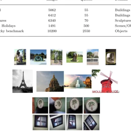
Table 2. Datasets for image retrieval benchmarking. The table shows the total number of images and queries of each dataset as well as the domain of search.
Dataset Images Queries Domain
Oxford 5062 55 Buildings
Paris 6412 55 Buildings
Sculptures 6340 70 Sculptures
INRIA Holidays 1491 500 Scenes/Objects
Kentucky benchmark 10200 2550 Objects
Figure 3. Samples from some retrieval benchmarks. First row, Sculptures; second row Paris; third and fourth rows Kentucky.
However, the kind of queries for these datasets (see Figure 3 for some examples) can be considered simpler than the queries in a generic instance search. In those datasets, the objects are usually the main part of the image and topics to retrieve are usually restricted to a particular domain.
3.1. TRECVid Instance Search
A generic instance search system should be able to find objects of an unknown category that may appear at any position within the images. TRECVID [63] is an international benchmarking activity that encourages research in video information
retrieval by providing a large data collection and a uniform scoring procedure for evaluation. The Instance Search task in TRECVID consists of finding 30 particular instances within 464 hours of video (a total of 224 video files, 300GB). For each query, 4 image examples are provided. A common procedure to deal with videos is to perform key frame extraction. For example, in our 2014 participation [64], the image dataset contained 647,628 image frames (66GB) by extracting 0.25 frames/second of the videos (which can be considered a low rate for a key frame extraction).
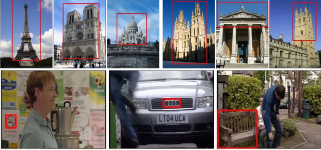
Figure 4. Query examples for TRECVID Instance search task [63]. Instance queries are divers: they can be logos, objects, buildings or people. Location and scale of the instances is also diverse.
There is no ground truth for the query images within the dataset and the number of examples per query is limited to 4 frames. Figure 4 shows an example of some of the 2014 TRECVid Instance Search queries.
Although promising results have shown the power of CNN representation on different retrieval benchmarks, results have mainly been reported for relatively small datasets, which are not sufficiently representative in terms of generalization or complexity of the queries for real world problem such as instance search in videos. Approaches that work well in small datasets may not work well in larger and more realistic datasets, such as TRECVID
4. Bag of Words Framework
The proposed pipeline for feature extraction uses the activations at different locations of a convolutional layer in a pre-trained CNN as local features. A CNN trained for a classification task is typically composed of a series of convolutional layers, followed by some fully connected layers, connected to a softmax layer that produces the inferred class probabilities. To obtain a fixed-sized output, the input image to a CNN is usually resized to be square. However, several authors using CNNs for retrieval [5,24] have reported performance gains by retaining the aspect ratio of the original images. We therefore discard the softmax and fully connected
layers of the architecture and extract CNN features maintaining the original image aspect ratio.
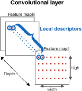
Each convolutional layer in the network has D different N ×M feature maps, which can be viewed asN×M descriptors of dimensionD. Each of these descriptors contains the activations of all neurons in the convolutional layer sharing the same receptive field. This way, theseD-dimensional features can be seen as local descriptors computed over the region corresponding to the receptive field of an array of neurons. With this interpretation, we can treat the CNN as a local feature extractor and use any existing aggregation technique to build a single image representation.
Figure 5. Re-interpretation of activation tensor into local descriptors
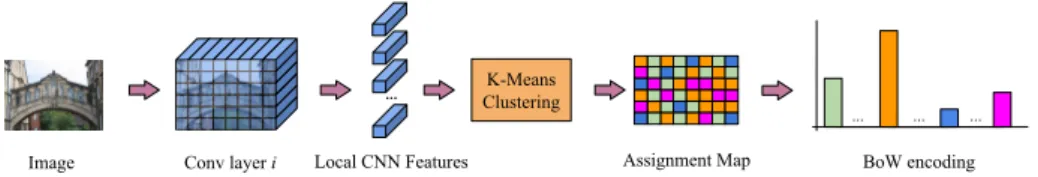
We propose to use the BoW model to encode the local convolutional features of an image into a single vector. Although more elaborate aggregation strategies have been shown to outperform BoW-based approaches for some tasks in the literature [26,65], BoW encodings produce sparse high-dimensional codes that can be stored in inverted indices, which are beneficial for fast retrieval. Moreover, BoW-based representations are faster to compute, easier to interpret, more compact, and provide all the benefits of sparse high-dimensional representations previously mentioned in Section 1.
BoW models require constructing a visual codebook to map vectors to their nearest centroid. We usek-means on local CNN features to fit this codebook. Each local CNN feature in the convolutional layer is then assigned its closest visual word in the learned codebook. This procedure generates theassignment map, i.e. a 2D array of sizeN×M that relates each local CNN feature with a visual word. The assignment map is, therefore, a compact representation of the image, which relates each pixel of the original image with its visual word with a precision of
W N,
H M
pixels, whereW and H are the width and height of the original image. This property allows us to quickly generate the BoW vectors of not only the full image, but also its parts. We describe the use of this property in our work in Section 5.
Figure 6 shows the pipeline of the proposed approach. The described bag of local convolutional features (BLCF) encodes the image into a sparse high dimensional descriptor, which will be used as the image representation for retrieval.
K-Means Clustering
BoW encoding ...
Conv layer i Local CNN Features Assignment Map
... ... ...
Image
Figure 6. The Bag of Local Convolutional Features pipeline (BLCF).
5. Image Retrieval
This section describes the image retrieval pipeline, which consists of an initial ranking stage, followed by a spatial reranking, and query expansion.
(a) Initial search: The initial ranking is computed using the cosine similarity
between the BoW vector of the query image and the BoW vectors of the full images in the database. We use a sparse matrix based inverted index and GPU-based sparse matrix multiplications to allow fast retrieval. The image list is then sorted based on the cosine similarity of its elements to the query. We use two types of image search based on the query information that is used:
• Global search (GS): The BoW vector of the query is built with the visual words of all the local CNN features in the convolutional layer extracted for the query image.
• Local search (LS): The BoW vector of the query contains only the visual words of the local CNN features that fall inside the query bounding box.
(b) Local reranking (R): After the initial search, the top T images in the
ranking are locally analyzed and reranked based on a localization score. We choose windows of all possible combinations of widthw∈ {W,W2,W4}and height h∈ {H,H2,H4}, whereW andH are the width and height of the assignment map. We use a sliding window strategy directly on the assignment map with 50% of overlap in both directions.
We additionally perform a simple filtering strategy to discard those windows whose aspect ratio is too different to the aspect ratio of the query. Let the aspect ratio of the query bounding box be ARq =
Wq
Hq andARw =
Ww
Hw be the aspect ratio of the window. The score for windowwis defined asscorew=
min(ARw,ARq)
max(ARw,ARq). All windows with a score lower than a thresholdthare discarded.
For each of the remaining windows, we construct the BoW vector represen-tation and compare it with the query represenrepresen-tation using cosine similarity. The window with the highest cosine similarity is taken as the new score for the image (score max pooling).
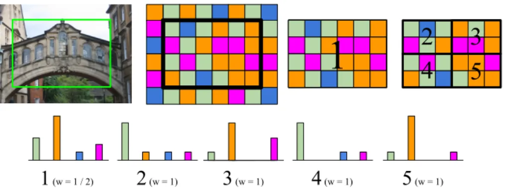
We also enhance the BoW window representation with spatial pyramid match-ing [66] with L= 2 resolution levels (i.e. the full window and its 4 sub regions). We construct the BoW representation of all sub regions at the 2 levels, and weight their contribution to the similarity score with inverse proportion to the resolution level of the region. The cosine similarity of a sub region rto the corresponding query sub region is therefore weighted by wr= 2(L1−lr), wherelris the resolution
1
2
4
3
5
1
(w = 1 / 2)2
(w = 1)3
(w = 1)4
(w = 1)5
(w = 1) Figure 7. Spatial pyramid matching on window locations.With this procedure, the top T elements of the ranking are sorted based on the cosine similarity of their regions to the query’s, and also provides the region with the highest score as a rough localization of the object.
(c) Query expansion:We investigate two query expansion strategies based on
global and local BoW descriptors:
• Global query expansion (GQE): The BoW vectors of the N images at the top of the ranking are averaged together with the BoW of the query to form the new representation for the query. GQE can be applied either before or after the local reranking stage.
• Local query expansion (LQE): Locations obtained in the local reranking step are used to mask out the background and build the BoW descriptor of only the region of interest of theN images at the top of the ranking. These BoW vectors are averaged together with the BoW of the query bounding box. The resulting BoW vector is used to perform a second search.
6. Experiments
6.1. Datasets
We use the following datasets to evaluate the performance of our approach:
Oxford Buildings [45] contains 5,063 still images, including 55 query images
of 11 different buildings in Oxford. A bounding box surrounding the target object is provided for query images. An additional set of 100,000 distractor images is also available for the dataset. We refer to the original and extended versions of the dataset as Oxford 5k and Oxford 105k, respectively.
Paris Buildings [46]contains 6,412 still images collected from Flickr including
query images of 12 different Paris landmarks with associated bounding box an-notations. A set of 100,000 images is added to the original dataset (Paris 6k) to form its extended version (Paris 106k).
TRECVid Instance Search 2013 [63] contains 244 video files (464 hours in
total), each containing a week’s worth of BBC EastEnders programs. Each video is divided in different shots of short duration (between 5 seconds and 2 minutes). We perform uniform key frame extraction at 1/4 fps. The dataset also includes
Figure 8. Query examples from the three different datasets. Top: Paris buildings (1-3) and Oxford buildings (4-6); bottom: TRECVid INS 2013.
30 queries and provides 4 still images for each of them (including a binary mask of the object location). In our experiments, we use a subset of this dataset that contains only those key frames that are positively annotated for at least one of the queries. The dataset, which we will refer to as the TRECVid INS subset, is composed of 23,614 key frames.
Figure 8 includes three examples of query objects from the three datasets.
6.2. Preliminary experiments
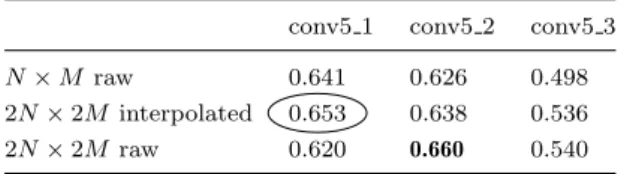
Feature extraction was performed using Caffe [67] and the VGG16 pre-trained network [68]. We extracted features from the last three convolutional layers (conv5 1, conv5 2 and conv5 3) and compared their performance on the Oxford 5k dataset. We experimented with different image input sizes: 1/3 and 2/3 of the original image. Following several other authors [1,24], weL2-normalize all local features, followed by PCA, whitening, and a second round of L2-normalization. The PCA models were fit on the same dataset as the test data in all cases.
Unless stated otherwise, all experiments used a visual codebook of 25,000 centroids fit using the (L2-PCA-L2 transformed) local CNN features of all images in the same dataset (1.7M and 2.15M for Oxford 5k and Paris 6k, respectively). We tested three different codebook sizes (25,000; 50,000 and 100,000) on the Oxford 5k dataset, and chose the 25,000 centroids one because of its higher performance.
Table 3 shows the mean average precision on Oxford 5k for the three different layers and image sizes. We also consider the effect of applying bilinear interpolation of the feature maps prior to the BoW construction, as a fast alternative to using a larger input to the CNN. Our experiments show that all layers benefit from feature map interpolation. Our best result was achieved using conv5 2 with full-size images as input. However, we discarded this configuration due to its memory requirements: on a Nvidia GeForce GTX 970, we found that feature extraction on images rescaled with a factor of 1/3 images was 25 times faster than on images
Table 3. Mean average precision (mAP) on Oxford 5k using different convolutional layers of VGG16, comparing the performance of different feature map resolutions (both raw and interpolated). The size of the codebook is 25,000 in all experiments.
conv5 1 conv5 2 conv5 3
N×M raw 0.641 0.626 0.498
2N×2M interpolated 0.653 0.638 0.536 2N×2M raw 0.620 0.660 0.540
twice that size. For this reason, we resize all images to 1/3 of their original size and use conv5 1 interpolated feature maps.
6.2.1. Center Prior Weighting
Inspired by the boost in performance of the Gaussian center prior in sum-pooled convolutional (SPoC) feature descriptors [1], we apply a weighting scheme on the visual words of an image to provide more importance to those belonging to the central part of the image. The weighting schemew(i, j) is described as:
w(i, j) =p 1
(i−c1)2+ (j−c2)2, (3)
where (i, j) represents the position of a visual word within the assignment map and (c1, c2) correspond to the center coordinated of the assignment map. w(i, j) min-max normalized to provide scores between 0 and 1. Table 3 shows the mean average precision on Oxford 5k for the three different layers and image sizes. All results are obtained using this weighting criteria; for conv5 1 in Oxford 5k, increases mAP from 0.626 to 0.653.
6.2.2. Layer Combination
We explore combining different layers in Oxford dataset. For that, layers were reshaped to have the same spatial dimensions by using bilinear interpolation. For instance, the last convolutional layer from VGG16, generates feature maps of dimensions (512,11,8) for an input size of (336,256). When combining with a lower layer such as conv5 1, pool5 maps have to be reshaped to double its dimensions (21,16) in order to be able to concatenate all the local features on a single volume of (1024,21,16). PCA-whitening reduces the dimensionality of the new local descriptors to 512D. Table 4 shows the effect in performance when combining different layers to conv5 1. We found that layer combination is potentially beneficial for our final representation (as found when combining con5 1 with pool5). Although since improvements found were marginally beneficial we discarded this approach in our pipeline.
6.3. Query augmentation
Previous works [17,69] have demonstrated how simple data augmentation strategies can improve the performance of an instance search system. Some of these apply augmentation strategies at the database side, which can be prohibitively costly
Table 4. Experiments layer combination conv5 1 conv5 2 conv5 3 pool5 mAP
X 0.653
X X 0.640
X X X 0.645
X X 0.671
Table 5. mAP on Oxford 5k for the two different types of query augmentation: the flip and the zoomed central crop (ZCC). 2×interpolated conv5 1 features are used in all cases.
Query + Flip + ZCC + Flip + ZCC GS 0.653 0.662 0.695 0.697 WS 0.706 0.717 0.735 0.743 LS 0.738 0.746 0.758 0.758
Original
Flip
ZCC
Flip + ZCC
Figure 9. The four query images after augmentation.
for large datasets. For this reason, we use data augmentation on the query side only. We explore two different strategies to enrich the query before visual search: a horizontal flip (or mirroring) and a zoomed central crop (ZCC) on an image enlarged by 50%.
Figure 9 shows an example of the transformations, which give rise to 4 different versions of the query image. The feature vectors they produce are added together to form a single BoW descriptor. Table 5 shows the impact of incrementally augmenting the query with each one of these transformations.
We find that all the studied types of query augmentation consistently improve the results, for both global and local search. ZCC provides a higher gain in perfor-mance compared to flipping alone. ZCC generates an image of the same resolution as the original, which contains the center crop at a higher resolution. Objects from the Oxford dataset tend to be centered, which explains the performance gain when applying ZCC.
6.4. Reranking and query expansion
We apply the local reranking (R) stage on the top-100 images in the initial ranking, using the sliding window approach described in Section 5. The presented aspect
Table 6. mAP on Oxford 5k and Paris 5k for the different stages in the pipeline introduced in Section 5. TheQaug additional columns indicate the results when the query is augmented with
the transformations introduced in Section 6.3.
Oxford 5k Paris 6k +Qaug +Qaug GS 0.653 0.697 0.699 0.754 LS 0.738 0.758 0.820 0.832 GS + R 0.701 0.713 0.719 0.752 LS + R 0.734 0.760 0.815 0.828 GS + GQE 0.702 0.730 0.774 0.792 LS + GQE 0.773 0.780 0.814 0.832 GS + R + GQE 0.771 0.772 0.801 0.798 LS + R + GQE 0.769 0.793 0.807 0.828 GS + R + LQE 0.782 0.757 0.835 0.795 LS + R + LQE 0.788 0.786 0.848 0.833
ratio filtering is applied with a threshold th = 0.4, which was chosen based on a visual inspection of results on a subset of Oxford 5k. Query expansion is later applied considering the top-10 images of the resulting ranking. This section evaluates the impact in the performance of both reranking and query expansion stages. Table 6 contains the results for the different stages in the pipeline for both simple and augmented queries (referred to asQaug in the table).
The results indicate that the local reranking is only beneficial when applied to a ranking obtained from a search using the global BoW descriptor of the query image (GS). This is consistent with the work by Tolias et al. [5], who also apply a spatial reranking followed by query expansion to a ranking obtained with a search using descriptors of full images. They achieve a mAP of 0.66 in Oxford 5k, which is increased to 0.77 after spatial reranking and query expansion, while we reach similar results (e.g. from 0.652 to 0.769). However, our results indicate that a ranking originating from a local search (LS) does not benefit from local reranking. Since the BoW representation allows us to effectively perform a local search (LS) in a database of fully indexed images, we find the local reranking stage applied to LS to be redundant in terms of the achieved quality of the ranking. However, the local reranking stage does provide with a rough localization of the object in the images of the ranking, as depicted in Figure 1. We use this information to perform query expansion based on local features (LQE).
Results indicate that query expansion stages greatly improve performance in Oxford 5k. We do not observe significant gains after reranking and QE in the Paris 6k dataset, although we achieve our best result with LS + R + LQE.
In the case of augmented queries (+Qaug), we find that this query expansion
is less helpful in all cases, which suggests that the information gained with query augmentation and the one obtained by means of query expansion strategies are not complementary.
Table 7. Comparison to state-of-the-art CNN representations (mAP). Results in the lower section consider reranking and/or query expansion.
Oxford Paris 5k 105k 6k 106k Nget al.[25] 0.649 - 0.694 -Razavianet al.[4] 0.844 - 0.853 -SPoC [1] 0.657 0.642 - -R-MAC [5] 0.668 0.616 0.830 0.757 CroW [24] 0.682 0.632 0.796 0.710 uCroW [24] 0.666 0.629 0.767 0.695 GS 0.652 0.510 0.698 0.421 LS 0.739 0.593 0.820 0.648 LS +Qaug 0.758 0.622 0.832 0.673 CroW + GQE [24] 0.722 0.678 0.855 0.797 R-MAC + R + GQE [5] 0.770 0.726 0.877 0.817 LS + GQE 0.773 0.602 0.814 0.632 LS + R + LQE 0.788 0.651 0.848 0.641 LS + R + GQE +Qaug 0.793 0.666 0.828 0.683
6.5. Comparison with the State-of-the-art
We compare our approach with other CNN-based representations that make use of features from convolutional layers on the Oxford and Paris datasets. Table 7 includes the best result for each approach in the literature. Our performance using global search (GS) is comparable to that of Ng et al. [25], which is the one that most resembles our approach. However, they achieve this result using raw Vector of Locally Aggregated Descriptors (VLAD) features, which are more expensive to compute and, being a dense high-dimensional representation, do not scale as well to larger datasets. Similarly, Razavian et al. [4] achieve the highest performance of all approaches in both the Oxford and Paris benchmarks by applying a spatial search at different scales for all images in the database. Such approach is prohibitively costly when dealing with larger datasets, especially for real-time search scenarios. Our BoW-based representation is highly sparse, allowing for fast retrieval in large datasets using inverted indices, and achieves consistently high mAP in all tested datasets.
We find the usage of the query bounding box to be extremely beneficial in our case for both datasets. The authors of SPoC [1] are the only ones who report results using the query bounding box for search, finding a decrease in performance from 0.589 to 0.531 using raw SPoC features (without center prior). This suggests that sum pooled CNN features are less suitable for instance level search in datasets where images are represented with global descriptors.
We also compare our local reranking and query expansion results with similar approaches in the state-of-the-art. The authors of R-MAC [5] apply a spatial search for reranking, followed by a query expansion stage, while the authors of CroW [24] only apply query expansion after the initial search. Our proposed approach also achieves competitive results in this section, achieving the best result for Oxford 5k.
6.6. Experiments on TRECVid INS
In this section, we compare the BLCF with the sum pooled convolutional features proposed in several works in the literature. We use our own implementation of the
uCroW descriptor from [24] and compare it with BLCF for the TRECVid INS subset. For the sake of comparison, we test our implementation of sum pooling using both our chosen CNN layer and input size (conv5 1 and 1/3 image size), and the ones reported in [24] (pool5 and full image resolution). For the BoW representation, we train a visual codebook of 25,000 centroids using 3M local CNN features chosen randomly from the INS subset. Since the nature of the TRECVid INS dataset significantly differs from that of the other ones used so far (see Figure 8), we do not apply center prior to the features in any case, to avoid down weighting local features from image areas where the objects might appear. Table 8 compares sum pooling with BoW in Oxford, Paris, and TRECVid subset datasets. As stated in earlier sections, sum pooling and BoW have similar performance in Oxford and Paris datasets. For the TRECVid INS subset, however, Bag of Words significantly outperforms sum pooling, which demonstrates its suitability for challenging instance search datasets, in which queries are not centered and have variable size and appearance. We also observe a different behavior when using the provided query object locations (LS) to search, which was highly beneficial in Oxford and Paris datasets, but does not provide any gain in TRECVid INS. We hypothesize that the fact that the size of the instances is much smaller in TRECVid than in Paris and Oxford datasets causes this drop in performance. Global search (GS) achieves better results on TRECVid INS, which suggests that query instances are in many cases correctly retrieved due to their context. Figure 12 shows the mean average precision of the different stages of the pipeline for all TRECVid queries separately. The global search significantly outperforms local search for most queries in the database. Figure 11 shows examples of the queries for which the local search outperforms the global search. Interestingly, we find these particular objects to appear in different contexts in the database. In these cases, the usage of the local information is crucial to find the query instance in unseen environments. For this reason, we compute the distance map of the binary mask of the query, and assign a weight to each position of the assignment map with inverse proportion to its value in the distance map. This way, higher weights are assigned to the visual words of local CNN features near the object. We find this scheme, referred to as weighted search (WS), to be beneficial for most of the queries, suggesting that, although context is necessary, emphasizing the object information in the BoW descriptor is beneficial.
We finally apply the local reranking and query expansion stages introduced in Section 5 to the baseline rankings obtained for the TRECVid INS subset. Since we are dealing with objects whose appearance can significantly change in different keyframes, we decided not to filter out windows based on aspect ratio similarity. Additionally, we do not apply the spatial pyramid matching, since some of the query instances are too small to be divided in sub regions. After reranking, we apply the distance map weighting scheme to the locations obtained for the top 10 images of the ranking and use them to do weighted query expansion (WQE).
Results are consistent with those obtained in the experiments in Oxford and Paris datasets: although the local reranking does not provide significant
Figure 10. Appearances of the same object in different frames of TRECVid Instance Search.
Figure 11. Top 5 rankings for queries 9072 (top) and 9081 (bottom) of the TRECVid INS 2013 dataset. 9069 9070 9071 9072 9073 9074 9075 9076 9077 9078 9079 9080 9081 9082 9083 9084 9085 9086 9087 9088 9089 9090 9091 9092 9093 9094 9095 9096 9097 9098 0 0.2 0.4 0.6 0.8 1 Av erage Pr e cision GS LS WS WS + GQE WS + R + WQE
Figure 12. Average precision of TRECVid INS queries.
improvements (WS: 0.350, WS + R: 0.348 mAP), the query expansion stage is beneficial when applied after WS (WS + GQE: 0.391 mAP), and provides significant gains in performance after local reranking (WS + R + GQE: 0.442 mAP) and after local reranking using the obtained localizations (WS + R + WQE: 0.452 mAP).
Table 8. mAP of sum pooling and BoW aggregation techniques in Oxford, Paris and TRECVid INS subset.
Oxford 5k Paris 6k INS 23k
BoW GS 0.650 0.698 0.323 WS 0.693 0.742 0.350 LS 0.739 0.819 0.295 Sum pooling (as ours) GS 0.606 0.712 0.156 WS 0.638 0.745 0.150 LS 0.583 0.742 0.097 Sum pooling (as in [24]) GS 0.672 0.774 0.139 WS 0.707 0.789 0.146 LS 0.683 0.763 0.120 7. Conclusion
We proposed an aggregation strategy based on Bag of Words to encode features from convolutional neural networks into sparse representations for instance search. We demonstrated the suitability of these bags of local convolutional features, achieving competitive performance with respect to other CNN-based represen-tations in Oxford and Paris benchmarks, while being more scalable in terms of index size, cost of indexing, and search time. We also compared our BoW encoding scheme with sum pooling of CNN features for instance search in the far more complex and challenging TRECVid instance search task, and demonstrated that our method consistently and significantly performs better. This encouraging result suggests that the BoW encoding, as a virtue of being high dimensional and sparse, is more robust to scenarios where only a small number of features in the target images are relevant to the query. Our method does, however, appear to be more sensitive to large numbers of distractor images than methods based on sum and max pooling (SPoC, R-MAC, and CroW). We speculate that this may be because the distractor images are drawn from a different distribution to the original dataset, and may therefore require a larger codebook to represent the diversity in the visual words better. Future work will investigate this issue.
References
[1] A. Babenko and V. Lempitsky. Aggregating local deep features for image retrieval. In
Proceedings of the IEEE international conference on computer vision, pages 1269–1277, 2015.
[2] A. Babenko, A. Slesarev, A. Chigorin, and V. Lempitsky. Neural codes for image retrieval. InComputer Vision–ECCV 2014, pages 584–599. 2014.
[3] A. Razavian, H. Azizpour, J. Sullivan, and S. Carlsson. CNN features off-the-shelf: an astounding baseline for recognition. InComputer Vision and Pattern Recognition Workshops, 2014.
[4] Ali S Razavian, Josephine Sullivan, Stefan Carlsson, and Atsuto Maki. Visual instance retrieval with deep convolutional networks. ITE Transactions on Media Technology and Applications, 4(3):251–258, 2016.
[5] G. Tolias, R. Sicre, and H. J´egou. Particular object retrieval with integral max-pooling of cnn activations. InInternational Conference on Learning Representations, 2016. [6] L. Xie, R. Hong, B. Zhang, and Q. Tian. Image classification and retrieval are one. In
Proceedings of the 5th ACM on International Conference on Multimedia Retrieval, pages 3–10. ACM, 2015.
[7] V. Nguyen, D. Nguyen, M. Tran, D. Le, D. Duong, and S. Satoh. Query-adaptive late fusion with neural network for instance search. InInternational Workshop on Multimedia Signal Processing (MMSP), pages 1–6, 2015.
[8] W. Zhang and C. Ngo. Topological spatial verification for instance search. IEEE Transac-tions on Multimedia, 17(8):1236–1247, 2015.
[9] X. Zhou, C. Zhu, Q. Zhu, S. Satoh, and Y. Guo. A practical spatial re-ranking method for instance search from videos. InInternational Conference on Image Processing (ICIP), 2014.
[10] C. Zhu and S. Satoh. Large vocabulary quantization for searching instances from videos. InInternational Conference on Multimedia Retrieval (ICMR), 2012.
[11] J. Sivic and A. Zisserman. Efficient visual search of videos cast as text retrieval. IEEE Transactions on Pattern Analysis and Machine Intelligence, 31(4):591–606, 2009. [12] P. Lennie. The cost of cortical computation.Current biology, 13(6):493–497, 2003. [13] W. E. Vinje and J. L. Gallant. Sparse coding and decorrelation in primary visual cortex
during natural vision. Science, 287(5456):1273–1276, 2000.
[14] H. J´egou, M. Douze, and C. Schmid. Improving bag-of-features for large scale image search.
International Journal of Computer Vision, 87(3):316–336, 2010.
[15] Y. Zhang, Z. Jia, and T. Chen. Image retrieval with geometry-preserving visual phrases. InComputer Vision and Pattern Recognition (CVPR), pages 809–816, 2011.
[16] T. Mei, Y. Rui, S. Li, and Q. Tian. Multimedia search reranking: A literature survey.
ACM Computing Surveys (CSUR), 46(3):38, 2014.
[17] R. Arandjelovi´c and A. Zisserman. Three things everyone should know to improve object retrieval. In2012 IEEE Conference on Computer Vision and Pattern Recognition, pages 2911–2918, June 2012.
[18] O. Chum, J. Philbin, J. Sivic, M. Isard, and A. Zisserman. Total recall: Automatic query expansion with a generative feature model for object retrieval. InIEEE International Conference on Computer Vision, Rio de Janeiro, Brazil, October 2007.
[19] A. Krizhevsky, I. Sutskever, and G. E. Hinton. Imagenet classification with deep convo-lutional neural networks. InAdvances in neural information processing systems, pages 1097–1105, 2012.
[20] J. Donahue, Y. Jia, O. Vinyals, J. Hoffman, N. Zhang, E. Tzeng, and T. Darrell. Decaf: A deep convolutional activation feature for generic visual recognition. InProceedings of the 31st International Conference on International Conference on Machine Learning -Volume 32, ICML’14, pages I–647–I–655. JMLR.org, 2014.
[21] J. Yosinski, J. Clune, Y. Bengio, and H. Lipson. How transferable are features in deep neural networks? InProceedings of the 27th International Conference on Neural Information Processing Systems, NIPS’14, pages 3320–3328, Cambridge, MA, USA, 2014. MIT Press. [22] Yunchao Gong, Liwei Wang, Ruiqi Guo, and Svetlana Lazebnik. Multi-scale orderless pooling of deep convolutional activation features. InComputer Vision–ECCV 2014. 2014. [23] Y. Liu, Y. Guo, S. Wu, and M. Lew. Deepindex for accurate and efficient image retrieval.
InInternational Conference on Multimedia Retrieval (ICMR), 2015.
[24] Y. Kalantidis, C. Mellina, and S. Osindero. Cross-dimensional weighting for aggregated deep convolutional features. InEuropean Conference on Computer Vision VSM Workshop, pages 685–701. Springer International Publishing, 2016.
[25] J. Yue-Hei Ng, F. Yang, and L. S. Davis. Exploiting local features from deep networks for image retrieval. InThe IEEE Conference on Computer Vision and Pattern Recognition (CVPR) Workshops, June 2015.
[26] H. J´egou, M. Douze, C. Schmid, and P. P´erez. Aggregating local descriptors into a compact image representation. In2010 IEEE Computer Society Conference on Computer Vision and Pattern Recognition, pages 3304–3311, June 2010.
for weakly supervised place recognition. InIEEE Conference on Computer Vision and Pattern Recognition, 2016.
[28] A. Jimenez, J. M. Alvarez, and X. Giro-i Nieto. Class-weighted convolutional features for visual instance search. In28th British Machine Vision Conference (BMVC), September 2017.
[29] B. Zhou, A. Khosla, A. Lapedriza, A. Oliva, and A. Torralba. Learning deep features for discriminative localization. InThe IEEE Conference on Computer Vision and Pattern Recognition (CVPR), June 2016.
[30] J. Deng, W. Dong, R. Socher, L. Li, K. Li, and L. Fei-Fei. Imagenet: A large-scale hierarchical image database. InComputer Vision and Pattern Recognition, 2009. CVPR 2009. IEEE Conference on, pages 248–255, June 2009.
[31] C. Reyes, E. Mohedano, K. McGuinness, and X. O’Connor, N.and Giro-i-Nieto. Where is my phone?: personal object retrieval from egocentric images. InProceedings of the first Workshop on Lifelogging Tools and Applications, pages 55–62. ACM, 2016.
[32] J. Pan, E. Sayrol, X. Giro-i Nieto, K. McGuinness, and N. O’Connor. Shallow and deep convolutional networks for saliency prediction. InProceedings of the IEEE Conference on Computer Vision and Pattern Recognition, pages 598–606, 2016.
[33] A. Salvador, X. Giro-i Nieto, F. Marques, and S. Shin’ichi. Faster R-CNN Features for Instance Search. InThe IEEE Conference on Computer Vision and Pattern Recognition (CVPR) Workshops, June 2016.
[34] S. Ren, K. He, R. Girshick, and J. Sun. Faster r-cnn: Towards real-time object detection with region proposal networks. IEEE Transactions on Pattern Analysis and Machine Intelligence, 39(6):1137–1149, June 2017.
[35] A. Gordo, J. Almaz´an, J. Revaud, and D. Larlus. End-to-end learning of deep visual representations for image retrieval. International Journal of Computer Vision, 124(2):237– 254, 2017.
[36] S. Chopra, R. Hadsell, and Y. LeCun. Learning a similarity metric discriminatively, with application to face verification. In2005 IEEE Computer Society Conference on Computer Vision and Pattern Recognition (CVPR’05), volume 1, pages 539–546 vol. 1, June 2005. [37] R. Hadsell, S. Chopra, and Y. LeCun. Dimensionality reduction by learning an invariant
mapping. In2006 IEEE Computer Society Conference on Computer Vision and Pattern Recognition (CVPR’06), volume 2, pages 1735–1742, 2006.
[38] Y. Taigman, M. Yang, M. Ranzato, and L. Wolf. Deepface: Closing the gap to human-level performance in face verification. InComputer Vision and Pattern Recognition (CVPR), 2014 IEEE Conference on, pages 1701–1708, June 2014.
[39] J. Bromley, I. Guyon, Y. LeCun, E. S¨ackinger, and R. Shah. Signature verification using a” siamese” time delay neural network. InAdvances in Neural Information Processing Systems, pages 737–744, 1994.
[40] N. Carlevaris-Bianco and R. M Eustice. Learning visual feature descriptors for dynamic lighting conditions. InIntelligent Robots and Systems (IROS 2014), 2014 IEEE/RSJ International Conference on, pages 2769–2776. IEEE, 2014.
[41] E. Simo-Serra, E. Trulls, L. Ferraz, I. Kokkinos, and F. Moreno-Noguer. Fracking deep convolutional image descriptors. arXiv preprint arXiv:1412.6537, 2014.
[42] S. Zagoruyko and N. Komodakis. Learning to compare image patches via convolutional neural networks. InProceedings of the IEEE Conference on Computer Vision and Pattern Recognition, pages 4353–4361, 2015.
[43] E. Hoffer and N. Ailon. Deep metric learning using triplet network. InInternational Workshop on Similarity-Based Pattern Recognition, pages 84–92. Springer, 2015. [44] F. Schroff, D. Kalenichenko, and J. Philbin. Facenet: A unified embedding for face
recognition and clustering. InProceedings of the IEEE Conference on Computer Vision and Pattern Recognition, pages 815–823, 2015.
[45] J. Philbin, O. Chum, M. Isard, J. Sivic, and A. Zisserman. Object retrieval with large vocabularies and fast spatial matching. In2007 IEEE Conference on Computer Vision and Pattern Recognition, pages 1–8, June 2007.
[46] J. Philbin, O. Chum, M. Isard, J. Sivic, and A. Zisserman. Lost in quantization: Improving particular object retrieval in large scale image databases. InProceedings of the IEEE
Conference on Computer Vision and Pattern Recognition, 2008.
[47] B. Zhou, A. Lapedriza, J. Xiao, A. Torralba, and A. Oliva. Learning deep features for scene recognition using places database. In Z. Ghahramani, M. Welling, C. Cortes, N. D. Lawrence, and K. Q. Weinberger, editors,Advances in Neural Information Processing Systems 27, pages 487–495. Curran Associates, Inc., 2014.
[48] S. Bell and K. Bala. Learning visual similarity for product design with convolutional neural networks.ACM Transactions on Graphics (TOG), 34(4):98, 2015.
[49] N. N. Vo and J. Hays. Localizing and orienting street views using overhead imagery, pages 494–509. 2016.
[50] J. Wang, Y. Song, T. Leung, C. Rosenberg, J. Wang, J. Philbin, B. Chen, and Y. Wu. Learning fine-grained image similarity with deep ranking. InProceedings of the IEEE Conference on Computer Vision and Pattern Recognition, pages 1386–1393, 2014. [51] F. Radenovi´c, G. Tolias, and O. Chum. CNN image retrieval learns from BoW: Unsupervised
fine-tuning with hard examples. InEuropean Conference on Computer Vision, pages 3–20. Springer International Publishing, 2016.
[52] H. Oh Song, Y. Xiang, S. Jegelka, and S. Savarese. Deep metric learning via lifted structured feature embedding. In Proceedings of the IEEE Conference on Computer Vision and Pattern Recognition, pages 4004–4012, 2016.
[53] J. Wan, D. Wang, S. C. H. Hoi, P. Wu, J. Zhu, Y. Zhang, and J. Li. Deep learning for content-based image retrieval: A comprehensive study. InProceedings of the 22nd ACM international conference on Multimedia, pages 157–166. ACM, 2014.
[54] K. Mikolajczyk and J. Matas. Improving descriptors for fast tree matching by optimal linear projection. In2007 IEEE 11th International Conference on Computer Vision, pages 1–8, Oct 2007.
[55] E. Ong, S. Husain, and M. Bober. Siamese network of deep fisher-vector descriptors for image retrieval. arXiv preprint arXiv:1702.00338, 2017.
[56] D. G. Lowe. Distinctive image features from scale-invariant keypoints. International Journal of Computer Vision, 60(2):91–110, 2004.
[57] W. Zhang and C. Ngo. Searching visual instances with topology checking and context modeling. InInternational Conference on Multimedia Retrieval (ICMR), pages 57–64, 2013.
[58] C. Zhu, H. J´egou, and S. Satoh. Query-adaptive asymmetrical dissimilarities for visual object retrieval. InInternational Conference on Computer Vision (ICCV), pages 1705– 1712, 2013.
[59] P. Felzenszwalb, D. McAllester, and D. Ramanan. A discriminatively trained, multiscale, deformable part model. InComputer Vision and Pattern Recognition (CVPR), pages 1–8, 2008.
[60] R. Arandjelovi´c and A. Zisserman. Smooth object retrieval using a bag of boundaries. In
IEEE International Conference on Computer Vision, 2011.
[61] H. J´egou, M. Douze, and C. Schmid. Hamming embedding and weak geometric consistency for large scale image search. Computer Vision–ECCV 2008, pages 304–317, 2008. [62]
[63] A. F. Smeaton, P. Over, and W. Kraaij. Evaluation campaigns and trecvid. InInternational Workshop on Multimedia Information Retrieval (MIR), 2006.
[64] K. McGuinness, E. Mohedano, Z. Zhang, F. Hu, R. Albatal, C. Gurrin, N. O’Connor, A. Smeaton, A. Salvador, X. Gir´o-i Nieto, and C. Ventura. Insight centre for data analytics (DCU) at TRECVid 2014: instance search and semantic indexing tasks. In2014 TREC Video Retrieval Evaluation Notebook Papers and Slides, 2014.
[65] F. Perronnin, Y. Liu, J. Snchez, and H. Poirier. Large-scale image retrieval with compressed fisher vectors. In2010 IEEE Computer Society Conference on Computer Vision and Pattern Recognition, pages 3384–3391, June 2010.
[66] S. Lazebnik, C. Schmid, and J. Ponce. Beyond bags of features: Spatial pyramid matching for recognizing natural scene categories. InComputer Vision and Pattern Recognition (CVPR), 2006.
[67] Y. Jia, E. Shelhamer, J. Donahue, S. Karayev, J. Long, R. Girshick, S. Guadarrama, and T. Darrell. Caffe: Convolutional architecture for fast feature embedding. InProceedings of
the 22nd ACM international conference on Multimedia, pages 675–678. ACM, 2014. [68] K. Simonyan and A. Zisserman. Very deep convolutional networks for large-scale image
recognition. arXiv preprint arXiv:1409.1556, 2014.
[69] P. Turcot and D. Lowe. Better matching with fewer features: The selection of useful features in large database recognition problems. InICCV WS-LAVD workshop, 2009.
![Figure 4. Query examples for TRECVID Instance search task [63]. Instance queries are divers:](https://thumb-us.123doks.com/thumbv2/123dok_us/381253.2542178/12.892.188.706.397.634/figure-query-examples-trecvid-instance-search-instance-queries.webp)