New evidence from the Medicare Advantage Program
By Jason Brown, Mark Duggan, Ilyana Kuziemko, William Woolston∗
To combat adverse selection, governments increasingly base pay-ments to health plans and providers on enrollees’ scores from risk-adjustment formulae. In 2004, Medicare began to risk-adjust cap-itation payments to private Medicare Advantage (MA) plans to reduce selection-driven overpayments. But because the variance of medical costs increases with the predicted mean, incentivizing en-rollment of individuals with higher scores can increase the scope for enrolling “over-priced” individuals with costs significantly be-low the formula’s prediction. Indeed, after risk adjustment, MA plans enrolled individuals with higher scores but lower costs condi-tional on their score. We find no evidence that overpayments were on net reduced.
JEL: H4, I1
Keywords: Medicare, Risk-Selection, Insurance Markets
Recent health care reforms have attempted to move away from the fee-for-service (FFS) payment model—which economists have long argued incentivizes over-provision of services—by paying providers or insurers fixed capitation pay-ments rather than reimbursing them for each service. The success of such reforms hinges on correctly aligning capitation payments with a patient’s expected cost. Otherwise, plans and providers will have incentives to cream-skim over-priced cases instead of competing on quality or cost.
To more accurately equate payments with expected costs, governments and other insurance sponsors have increasingly turned to “risk adjustment”—setting payments to insurers or providers to take account of an individual’s past and current health conditions. For example, the Affordable Care Act of 2010 (ACA) ∗ Brown: U.S. Treasury, Office of Economic Policy, 1500 Pennsylvania Ave. NW, Washington, DC, 20005, [email protected]; Duggan: University of Pennsylvania, The Wharton School, Department of Business Economics and Public Policy, 3620 Locust Walk , Philadelphia, PA 19104, [email protected]; Kuziemko: 602 Uris Hall, Columbia University, New York, NY 10027, [email protected]; Woolston: J.P. Morgan Chase, 270 Park Avenue, New York, NY, 10017. Sur-name2: affiliation2, address2, email2. We thank Richard Boylan, Doug Bernheim, Sean Creighton, David Cutler, Liran Einav, Randy Ellis, Zeke Emanuel, Gopi Shah Goda, Jonathan Gruber, Caroline Hoxby, Seema Jayachandran, Larry Katz, Robert Kocher, Jonathan Kolstad, Amanda Kowalski, Alan Krueger, Joe Newhouse, Elena Nikolova, Christina Romer, Shanna Rose, Karl Scholz, Jonathan Skinner, and Luke Stein and seminar participants at Brown, Columbia, Cornell, Harvard, Houston, Northwestern, MIT, Princeton, RAND, Rice, Stanford, USC, U.S. Treasury Department, Wharton, Wisconsin, Yale, and the NBER Health Care meetings for helpful comments and feedback. We thank Nadia Tareen and Boris Vabson for their outstanding research assistance. Views expressed here are solely those of the authors and not of the institutions with which they are affiliated, and all errors are our own.
relies heavily on risk adjustment.1 However, empirical research on these attempts to risk-adjust has been limited.2
In this paper, we provide an assessment of the largest risk-adjustment effort to date in the U.S. health care sector—Medicare’s risk adjustment of capitation payments to private Medicare Advantage (MA) plans, which the ACA suggests as the model for risk adjustment in the state-run insurance exchanges—on selection into MA plans and on the government’s total cost of financing Medicare bene-fits. Since the 1980s, Medicare enrollees have been able to enroll in either the traditional fee-for-service (FFS) program or in an MA plan, which can provide additional services but must cover the basic benefits guaranteed by traditional Medicare. For an individual in an MA plan, the government pays the plan a capitation payment meant to cover the cost of providing her Medicare benefits. Today, more than one-fourth of Medicare’s 51 million enrollees receive their care through a private MA plan.
Before 2004, an MA enrollee’s capitation payment was, essentially, based on the average cost of FFS enrollees with the same demographic characteristics in her county and was not adjusted for health conditions. Despite regulations requiring MA plans to offer the same plan at the same price to all Medicare beneficiaries in its geographical area of operation, researchers found that less costly individuals were much more likely to enroll in an MA plan.3 Reacting to this evidence of “differential payments” to MA plans—payments in excess of the expected cost of covering a beneficiary in traditional FFS—in 2004 Medicare began to base capi-tation payments on an individual’s “risk score,” generated by a risk-adjustment formula accounting for more than seventy disease conditions.
We develop a simple model to show that plans’ endogenous response to risk adjustment can undo the intended goal of reducing overpayments and test it using data from the Medicare Current Beneficiary Survey (MCBS). Before risk adjustment, MA plans had an incentive to enroll individuals who were low cost on all dimensions. After risk adjustment, plans no longer need to avoid beneficiaries with conditions included in the formula. In a difference-in-differences model, we show that, relative to individuals who remain in FFS, risk scores of those joining MA increase after risk adjustment, consistent with our model’s predictions.
However, our model emphasizes how selection can take place on different mar-1Approximately 25 million people are projected to join the insurance exchanges established by the ACA, in which private insurers will receive capitation payments adjusted for enrollees’ health status.
2There is a large, mostly theoretical or statistical, literature on risk adjustment, and Van de ven and Ellis (2000) and Ellis (2008) serve as excellent reviews. Recently, work has focused on “optimal” risk adjustment, following Glazer and McGuire (2000) who argue that mere predictive models (such as the one used by Medicare, on which we focus the empirical work) are fundamentally misguided because formula coefficients need to be chosen for their incentive, not predictive, properties. However, as noted by Ellis (2008), predictive models are by far the most common risk adjustment models in use today, and thus determining their effect on selection and costs is a central policy question. On the empirical side, Bundorf, Levin and Mahoney (2012) provides estimates on the welfare gains to risk adjustment of health insurancepremiums.
3See, e.g., Langwell and Hadley (1989), Physician Payment Review Commission (1997), Mello et al. (2003) and Batata (2004).
gins. While risk adjustment indeed decreases plans’ scope for advantageous se-lection along the dimensionsincluded in the formula, it increases the incentive to find individuals who are positively selected along dimensionsexcluded from the formula and are thus “cheap for their risk score.” Indeed, as the model predicts, we find that actual costs conditional on the risk score of those joining MA fall substantially after 2003, relative to those remaining in FFS.
Finally, the model makes clear that the former effect (the decrease in selection along dimensions included in the formula) can be more than offset by the latter effect (the increased selection conditional on the risk score). The key insight is that because the variance of medical costs increases with the expected mean, there are more cases of extremely high overpayments among those with high risk scores. Figure 1, which plots average medical costs along with the 10th and 90th percentile, shows how the variance of medical costs increases with a patient’s risk score. Given that costs are bounded below by zero, overpayments to those with a risk score of 0.5 are bounded above by $3,500, whereas if plans can manage to avoid the costliest ten percent of enrollees with a risk score of two (five), their overpayments for this group would average over $5,000 ($9,000).4
Due to this increase in variance, the ability of firms to enroll individuals with costs substantially below the formula’s prediction—whether through targeted advertising or designing benefits packages that differentially appeal to certain people—can actually increase after risk adjustment, and with it the government’s total cost of financing the Medicare program. To take but one example from our data, pre-risk-adjustment, Hispanics were roughly $1,200 cheaper on aver-age than their (non-risk-adjusted) capitation payments; after risk adjustment, Hispanics with a history of congestive heart failure (one of the most common conditions included in the risk formula) are on average $3,500 cheaper than their (risk-adjusted) capitation payments. Intuitively, before risk adjustment MA plans fished in a pond of relatively healthy enrollees with little cost variance. Risk ad-justment allows them to fish in a pond of enrollees who have higher costs on average but also highlyvariablecosts. Indeed, we find that after risk adjustment, overpayments are higher, an increase equal to roughly nine percent of average Medicare per capita spending.
This counterintuitive consequence of risk adjustment has, to the best of our knowledge, not been noted by other researchers, but is related to the literature on the unintended consequences of increasing the specificity of incomplete contracts. By selecting individuals with low costs conditional on their risk scores, MA firms’ behavior is analogous to the worker who focuses on the contractable task to the detriment of other tasks (as in Holmstrom and Milgrom, 1991) or the instructor who “teaches to the test” at the expense of other educational goals (as in Lazear, 2006). More generally, our results suggest that using additional information to determine prices can sometimes aggravate problems associated with asymmetric 4For these calculations, we use average FFS costs as an estimate for plan per-enrollee payments. The next section discusses modifications to this formula over time.
information, as in Einav and Finkelstein (2011).
While we find little evidence that risk adjustment accomplished the goal of re-ducing overpayments, we also examine whether the increased overpayments led to greater consumer or producer surplus. Our results suggest little to no improve-ment in several alternative measures of beneficiary satisfaction and quality of care. These results are consistent with recent research regarding the incidence of MA reimbursement generosity (Cabral, Geruso and Mahoney, 2013), with additional advertising expenditures absorbing much of the additional Medicare spending (Mehrotra, Grier and Dudley, 2006 and Duggan, Starc and Vabson, 2013). Per-haps because of these additional marketing costs, benefits to plans were also lim-ited, with CMS actually increasing plan reimbursement to cushion the expected negative effect of risk adjustment on insurers’ profits.
The remainder of the paper is organized as follows. Section I provides back-ground information on the MA program and the risk-adjustment formula Medi-care currently uses. Section II presents the intuition and results from the model. Section III describes the data. Sections IV and V present the empirical results on selection and differential payments, respectively. Section VI explores poten-tial mechanisms by which MA plans might be able to differenpoten-tially select certain enrollees. Section VII explores the welfare consequences of risk adjustment and discusses ways to improve it, and Section VIII concludes.
I. Medicare Advantage capitation payments and risk adjustment
Since the 1980s, Medicare enrollees have had the choice between the traditional FFS program and private MA plans (previously known as Medicare+Choice or Part C plans). The evolution of MA enrollment as a share of total Medicare enrollment during our sample period is plotted in Appendix Figure 1.
Plans must accept all applicants residing in their areas of operation and provide benefits that are covered under traditional Medicare. MA plans have consider-able latitude in creating their hospital and physician networks. Many offer extra benefits such as vision care, dental care, and gym memberships. Plans can also charge a monthly premium, reduce enrollees’ Medicare Part B premiums, or vary copayments.
The Medicare program pays MA plans a fixed capitation payment to cover these costs (excluding hospice care, which FFS covers), and plans are, essentially, the residual claimants if actual costs are above or below the capitation payment. Since 2006, Medicare Part D has provided enrollees coverage for prescription drugs, though all of our analysis will focus on Part A (hospital and inpatient) and B (physician and outpatient), as these are the services MA plans are required to provide.5
The capitation payment to an MA plan for covering an individual is based on the estimated Part A and B payments had FFS Medicare covered her directly. During 5MA plans that provide prescription drug coverage receive a separate capitation payment in return.
the 1980s and 1990s, the Center for Medicare and Medicaid Services (CMS)—the agency that administers Medicare—used a “demographic model” to perform this estimation, so-called because it included primarily demographic variables (gender, age, and disability, Medicaid and institutional status) as opposed to disease or health conditions. The demographic model would output a “risk score” (with mean one) that when multiplied by a county-level “benchmark” would determine the capitation payment. Then as now, CMS did not require MA plans to report cost or claims data, so it used FFS data to regress total Part A and B spending on these demographic factors, finding that one percent of FFS expenditures were explained by the risk score (Pope et al., 2004).
In response to research showing that MA plans enrolled beneficiaries who were significantly cheaper than the demographic model predicted, CMS revised its risk-adjustment procedure.6 In 2000, CMS made ten percent of capitation payments dependent on inpatient claims data, raising the effectiveR2 of the formula from 1.0 to 1.5 percent. More significantly, in 2004—which for simplicity we term the “start” of risk adjustment—CMS introduced the hierarchical condition categories (HCC) model, still in use today. The HCC model, like the demographic model, uses data from the FFS population to predict FFS costs in the following year, but instead of relying only on demographic data, it also accounts for the disease conditions included on FFS providers’ claims. The model distills the roughly 15,000 ICD-9 codes that providers can list on claims into seventy disease-category indicator variables, the most common of which are described in Appendix Table 1. By definition, these variables are the same whether a person has 1 or 100 claims for a certain condition. Initially, the HCC model was blended with the demographic model, and accounted for 30, 50, 75, and 100 percent of the total risk score in, respectively, 2004, 2005, 2006, and 2007 or later. To help plans adjust to the new system, CMS increased payments across the board to MA plans after risk adjustment (we discuss the potential effects of these payments in the next section).
CMS found that within the FFS population, the HCC risk score explained eleven percent of FFS expenditures the following year (Pope et al., 2004). New-house, Buntin and Chapman (1997) and Van de ven and Ellis (2000) survey the literature and conclude that the lower bound on the percent of expenditure vari-ation that insurers are able to predict is between 20 and 25 percent, suggesting there is still room for risk selection even if the model performs as well on the MA population as it does on the FFS population. Similarly, reports commissioned by CMS in 2000 and 2004 (Pope et al., 2000 and Pope et al., 2004) and more recent work (Frogner et al., 2011) have found that—again, looking only at the FFS population—the formula systematically under-predicts spending for those with the most serious health conditions.
6Estimates from Langwell and Hadley (1989), Physician Payment Review Commission (1997), Mello et al. (2003) and Batata (2004) suggest that individuals switching from traditional FFS to MA had medical costs between 20 and 37 percent lower than observably similar individuals who remained in FFS.
It is worth noting that, for at least three reasons, the spending prediction from the HCC model is likely to perform worse on the MA population than on those in FFS. First, out-of-sample prediction is more difficult than in-sample predic-tion. Second, CMS has found that MA plans exhibit greater “coding intensity” in documenting disease conditions than do FFS providers. For example, what an FFS provider codes as “diabetes” an MA plan might code “diabetes with compli-cations,” thus increasing the enrollee’s capitation payment (CMS 2010). Third, MA plans may target beneficiaries for whom the formula over-predicts costs. In-deed, as the model in the next section demonstrates, risk adjustment incentivizes insurers to enroll individuals whom they expect to have low costsconditional on their risk score.
II. Theoretical framework
Our model of how plans will respond to risk adjustment relies on a simple, under-appreciated fact about medical costs: as its expectation rises, so does the variance around that expectation. One might paraphrase and say that healthy people are all alike, but sick people are each sick in their own way.
Before risk adjustment, when plans were roughly getting about $8,000 per en-rollee, regardless of medical history, it made little financial sense for a plan to enroll someone with a risk-score of, say, five, meaning expected costs of $40,000. Yet, as Figure 1 shows, because of the substantial variance such an individual exhibits, post risk-adjustment the margin between the capitation payment for these individuals and actual costs can be significant if plans can engage in even modest risk selection. As noted in the introduction, merely avoiding the costliest ten percent of enrollees within a risk group nets substantial margins (e.g., roughly $7,500 on average for those with risk scores between three and four).
The idea of large potential margins among those with high risk scores is cap-tured nicely in the below quote from Thomas Scully, the director of CMS from 2001 to 2003 and currently a general partner in a private equity firm focusing on health care:
If you get paid $10,000 per year for everybody [as in the pre-risk-adjustment regime], you are going to find healthy people and avoid the sick people. Well, now we have risk adjustment in Medicare...[Insurance plans] want to find a $50,000 patient because . . . you can’t make an $8,000 margin when Medicare is paying you $8,000. Risk adjust-ment has totally flipped all of the incentives in Medicare for insurance companies.7
The quote emphasizes that, perhaps ironically, the margin between capitation payments and medical costs (i.e., differential payments) can actually increase 7From an April 28, 2011 conference at Columbia Business School. A full video of his remarks can be found athttp://www.youtube.com/watch?v=r_apgZpHhh8&feature=relmfu.
post-risk adjustment, now that plans can “fish” in a high-variance, high-expected-mean “pond.”
A. Illustrating the theory with a simple example
We begin with a simple three-type example that can show all the key insights of the model, and then describe how these results are generalized in the mathe-matical Appendix.
Basic set-up. There are three types of individuals, one of whom is “healthy” and two of whom are “sick.” Each type represents a third of the population. To fix ideas, type A is “healthy” and has no documented health conditions. He has expected costs of 5 were he to be covered directly by FFS, and there is no cost variation within members of type A: recall, healthy people are all alike. “Sick” types have cancer, and are not all alike. Type B has cancer that is in remission and has costs of 6; type C is receiving chemotherapy and has costs of 13. Table 1 displays this information. For simplicity, we assume that medical costs of treating each type is the same in FFS as for an MA plan.8
Before risk adjustment, capitation payments are set equal to average FFS costs across all types, or 8 (5+6+133 ). After risk adjustment, the government pays plans the average cost in eachrisk category—that is, no conditions (type A) and cancer (types B and C). For simplicity, we assume that the risk score is equal to average cost, so the risk score for those with no conditions (type A) equals 5 and the risk score for those with cancer (types B and C) equals 6+132 = 9.5. Note that risk adjustment is “payment-neutral” in the sense that, if the entire Medicare population joined MA, total capitation payments would be the same before and after risk adjustment, 3×8 = 24 and 5 + 9.5 + 9.5 = 24, respectively.
While MA plans must accept any individual who wishes to join, we assume that a plan can—at some cost—influence the characteristics of its enrollees. These screening costs could include targeted advertising or additional benefits that ap-peal to certain groups. We assume that it is costlier to screen within a risk category thanacross categories. Applying these assumptions to our example, we set screening costs for type A individuals at just 1 while costs for type B (or C) individuals are 2. Put another way, it costs less to attractgenerally healthy individuals than to attract relatively healthy cancer patients. However, the cost of screening within a risk category falls with the the category’s mean cost. In our example, the cost of screeningamong Type A individuals is infinite, as “healthy people are all alike.” The cost of screening among those in the cancer risk cate-gory is positive but finite. If, instead, firms decline to influence their enrollment and merely open their door to all comers, screening costs are assumed to be zero.
Enrollment before risk adjustment. Profits are defined as capitation
payment less medical and screening costs (if any). If plans do not screen, they 8In practice, MA plans may affect the utilization of health care or negotiate different prices with providers.
make zero expected profits, as capitation payments and medical costs are equal in expectation. If they screen, as Table 1 shows, profits pre-risk-adjustment are 2, 0 and -7 when plans selectively enroll types A, B and C, respectively. We assume that insurers only enroll profitable individuals, so plans will choose to selectively enroll type A individuals and earn profits of 2.
Enrollment after risk adjustment. Again, if plans do not screen, they
make zero expected profits because both pre- and post-risk adjustment, medical costs and capitation payments are equal in expectation. If they screen, profits are -1, 1.5 and -5.5 for selectively enrolling types A, B and C, respectively. Plans thus enroll type B and earn profits of 1.5.
Results. The first outcome of note is that therisk scores of those enrolled in MA increase after risk adjustment, specifically from 5 (A’s risk score) in the pre-period to 9.5 (B’s risk score) in the post-pre-period. Intuitively, post risk adjustment there is no longer a penalty for enrolling individuals with high risk scores, so plans no longer expend the screening costs to avoid such individuals. We term selectively enrolling those with low risk-scores “extensive-margin screening” and our model thus predicts that it falls after risk adjustment.
The second outcome of note is that for those enrolled in MA, medical costs conditional on the risk score fall after risk adjustment. Specifically, in the pre-period, medical costs less the risk score were 5−5 = 0, falling to 6−9.5 =−3.5 in the post-period. The key to this result is that within-risk-score screening costs fall with the risk score itself. To paraphrase the quote, it is impossible to find someone with a $10,000 margin when they have a low risk score and thus, say, an $8,000 capitation payment. But, for patients with high risk scores, such a margin is possible because of the high variance. Again, in our example, the cost of screening within Type A (risk score= 5) is infinite, as no variation exists.9 We term selectively enrolling those with costs below their risk score “intensive-margin selection.”
A third outcome is that risk adjustment would have reduced differential pay-ments had the population joining MA remained fixed. In our example, only Type A joins MA before risk adjustment, and risk adjustment reduces differential pay-ments for this population to zero.
A fourth outcome from our example is that the government’s differential pay-ments (capitation paypay-ments less medical costs) actually rise under risk adjust-ment. In the pre-period, differential payments were 8−5 = 3, rising to 9.5−6 = 3.5 in the post-period.
A fifth outcome is that profits fall. Because risk adjustment changes the screen-ing costs that insurers pay, differential payments and plan profits need not move together. In our original example, profits actually fall from 2 to 1.5 given the increased screening costs. As we do not have data on MA-specific insurer profits, 9We make this assumption so as not to need four types to illustrate the point, but as we show in the Appendix, the result of increasing intensive-margin selection does not depend on the particular screening costs we choose here.
we cannot directly test this result, but we return to it when we discuss welfare in Section VII.10
In the appendix, we go from three types to a continuum of types and allow the predictive power of risk adjustment to vary continuously as well. As we show, all five results from our three-type discrete set-up hold, with an important exception: the effect of risk adjustment on overpayments is ambiguous. The reason for the ambiguity reinforces the main theme of the paper: the success of risk adjustment depends crucially on how much medical cost variance increases with the risk score. Suppose in our example that instead of ranging from 6 to 13, the costs of those with cancer range only from 7 (type B) to 12 (type C). In the post-period, it is still the case than plans only enroll type B. Our two selection results hold: for those in MA, risk scores rise from 5 to 9.5 (“extensive-margin” selection falls) and costs less the risk score falls, in this case from 5−5 = 0 to 7−9.5 = −2.5 (“intensive-margin” selection increases). However, risk adjustment in this case has accomplished its goal of reducing the government’s differential payments, from 3 in the pre-period to 9.5−7 = 2.5 in the post-period.
B. Discussion of assumptions
First, a central though seemingly innocuous assumption of the model ispayment neutrality, that if MA plans were to enroll all Medicare enrollees (or a random sam-ple thereof), total payments would be the same before and after risk adjustment. If, instead, risk adjustment is accompanied by an increase in what we term “statu-tory” overpayments—that is, overpayment related to the government’s decision to systematically overpay MA plans on average, even absent risk-selection—then our predictions need not hold. Suppose that along with risk adjustment, Medicare decided to increase all capitation payments by twenty percent, as we illustrate in Appendix Table 2. Results are unchanged in the pre-period, but now plans can either engage in screening, in which case it is most profitable to differentially enroll type B for a profit of 9.5∗1.2−6−2 = 3.4. Or, they can open their doors to all comers and gain 1.2∗(5 + 9.5 + 9.5)−5−6−13 = 4.8, as they no incur no screening costs. As such, if risk adjustment is accompanied with large increases in statutory overpayments, plans will at some point lose any incentive to find those who are cheap conditional on their risk score.
This point is empirically important because statutory overpayments have in-creased substantially over time. From 2001-2003, MA plans would receive 104 percent of FFS costs, absent any risk-selection, as policy-makers began to set county “benchmarks” above average county FFS spending.11 From 2004-2006 10Finally, we note that our model yields ambiguous predictions on how the average medical costs of MA enrollees should change. On the one hand, after risk adjustment MA enrollees will have higher risk scores. On the other hand, their costs conditional on their score will fall. In the Appendix, we show that the second effect can dominate and that risk adjustment can cause average costs of MA enrollees to fall. We hasten to add that this result is not general—indeed, in our example medical costs among those in MA increase from 5 to 6—but is possible.
(our post-period), these payments rose to 108 percent, both because the county “benchmarks” increased at a faster rate than did FFS spending and because CMS explicitly gave MA plans so-called “budget neutrality” payments (plans ar-gued they would need these extra payments to compensate them for the expected revenue loss due to risk adjustment). From 2007-2009, benchmark increase and budget-neutrality payments led to statutory overpayments between 113 and 114 percent.12 For this reason, we choose a rather short post-period, when the change in these statutory overpayments is still relatively limited. Consistent with the pre-diction that once statutory overpayments are sufficiently large plans will be less selective, MA enrollment between 2006 and 2010 increased by 63 percent (from 6.8 million to 11.1 million).13
Second, our assumptions regarding the manner in which screening costs vary across risk categories are obviously central to the model, but we are rather silent on what, in practice, these screening costs might entail. How do plans differen-tially attract “over-priced” consumers? We empirically explore some possibilities in Section VI. Strictly speaking, how they do so is irrelevant to the government’s bottom line, which is our main focus. Of course, it is highly relevant to consumer surplus, which we explore when we discuss welfare in Section VII.
Third, we are also rather silent on plan competition. We believe competition is likely second-order in determining the cost to the government, as MA capitation payments are set by the risk-adjustment formula and not competitive bidding. Again, however, competition likely affects how producer and consumer surplus change as a result of risk adjustment and so we explore this topic in Section VII.14
III. Data
Our empirical work relies chiefly on individual-level data from the Medicare Current Beneficiary Survey (MCBS) Cost and Use series from 1994 to 2006. The MCBS links CMS administrative data to surveys from a nationally representative sample of roughly 11,000 Medicare enrollees each year. It also provides complete claims data from hospital admissions, physician visits, and all other Medicare-than FFS and thus systematically set benchmarks at 95 percent of county FFS per capita spending. The earlier work we cited suggests that plans were still able to enroll individuals who were on average less than 95 percent of average FFS costs, meaning net overpayments were still high, but during this period none of the net overpayments were due to statutory overpayments, unlike recent years.
12All figures come from various MedPAC reports, which annually document statutory overpayments. 13Indeed, while in Section IV we document evidence of significant intensive-margin screening from 2004 to 2006, evidence from more recent years is mixed. In its 2012 annual report to Congress, MedPAC, citing a working-paper version of our study, found nearly identical levels of intensive-margin selection levels using the universe of Medicare enrollees in 2007 and 2008 (MedPAC, 2012). Results from McWilliams, Hsu and Newhouse (2012), however, suggest that risk-selection decreased in 2007-2008 relative to 2004-2006, consistent with higher statutory overpayments diminishing risk-selection incentives.
14Past studies have explored consumer surplus, profits, and competition in the MA market, though all are from the pre-risk-adjustment era. Hall (2011) finds that between 1999 and 2002, annual consumer surplus surpassed $12 billion. Town and Liu (2003) estimate that between 1993 and 2000, the MA program generated over $18 billion in consumer surplus, and nearly three times that amount in insurer profits.
covered provider contact for all FFS enrollees in the sample, totaling about 0.5 million claim-level observations annually. The MCBS follows a subsample of respondents for up to three or four years, thus creating a mix of cross-sectional and panel data. During our sample period, the data comprise more than 55,000 unique individuals and 150,000 person-year observations.15
The MCBS records whether an individual is in an MA plan or FFS each month he is in the sample. As noted in Section I, MA plans do not submit claims or costs to CMS, and thus the MCBS only contains claims and health care cost data for those in FFS. Otherwise, all demographic and survey data are recorded for both MA and FFS enrollees. Consistent with past work, we find that, relative to their FFS counterparts, MA enrollees are more likely to live in metro areas, are less likely to be on Medicaid or Social Security Disability Insurance (SSDI) and, conditional on not being on SSDI, are younger.
Some of the key predictions from the theoretical framework in Section II involve enrollees’ risk scores, which the MCBS does not report. We obtained risk scores from 2004 to 2006 for all MCBS respondents directly from CMS. However, testing two of our key predictions also involves knowing what individuals’ risk scores
would have been in the earlier years had the HCC formula been in place, which we must generate ourselves. As described above, an individual’s risk score in year
t is based on diagnoses documented on claims from year t−1. As such, using CMS’s algorithm for converting claims data into risk scores, we simulate the risk score for all MA enrollees the year immediately after they switch from FFS. As we know the actual risk scores from 2004 to 2006, we check our simulation in these years: the correlation between our simulated risk scores and CMS’s actual scores is more than 0.96.
The need to calculate HCC scores in the pre-period means we limit some of our analysis to those individuals who were in FFS all twelve months of a baseline year, so that we observe their complete claims history that year. Table 2 shows the number of observations who are in FFS in yeartand in MA in year t+ 1, as well as the number who are in FFS both years, and how these numbers change across our sample period. Of the more than 85,000 cases in which we observe a person in both yeartand yeart+ 1, more than 1,500 involve switches from FFS to MA. One limitation of the focus on FFS-to-MA switchers is that it ignores those who join MA immediately upon their Medicare eligibility. Our MCBS data demonstrate, however, that more than 3-in-4 new MA enrollees come from FFS, as opposed to joining when first enroll in Medicare.16
15We exclude the 0.25 percent of enrollees whose Medicare eligibility is based on having end-stage-renal disease, as different MA rules apply to them. We also exclude the roughly 2 percent of observations in which the person joins the MCBS in the middle of the year because much of their data are imputed. 16In Table 2, we show that 2.1 percent of FFS recipients switch into MA the next year. With an average of 35 million in Medicare FFS during our study period, that represents 735,000 per year. During our period, about 2 million individuals become eligible for Medicare each year, and about 12 percent (240,000) of them are enrolled in MA in that first year.
IV. How did selection patterns into MA change after risk adjustment?
In this section, we empirically test our model’s predictions regarding the effect of risk adjustment on both extensive-margin selection (did MA beneficiaries’ risk scores rise?) and intensive-margin selection (did their costs conditional on their risk score fall?).
A. Quantifying the selection incentives created by the HCC model
Col. (1) of Table 3 presents the average difference between the HCC-based capitation payment and the traditional demographic-based capitation payment using our MCBS data, with this difference broken down by percentiles of the HCC risk score.17 Mechanically, capitation payments must, on average, rise under the HCC formula for those with higher risk scores, and col. (1) merely presents the magnitudes. For example, the HCC capitation payment would, on average, pay about $3,000 less than the demographic-based capitation payment for individuals with HCC scores in the lowest quartile, but would pay roughly $7,000 more for the individuals in the top quartile.
Col. (1) suggests that insurers would have an incentive to increase risk scores over the entire risk score distribution, but col. (2), which reports actual costs minus the HCC capitation payment, shows that doing so would not always be profitable. For example, individuals with the highest one percent of risk scores represent, on average, a nearly $6,000 loss to an MA plan, consistent with the research cited earlier showing that the HCC formula under predicts costs for enrollees with the most severe disease conditions. Plans might thus be reluctant to draw from the extreme right tail of the risk-score distribution.
Though not shown in the table, we also calculate that the share of individ-uals who have actual baseline costs less than their risk scores would predict is 77 percent under both the demographic and the HCC model. This result arises because of the extreme right-skew of health costs—the vast majority of the distri-bution falls below the mean (or conditional mean, in the case of risk adjustment). Thus, risk adjustment does not actually decrease the number of individuals who are “over-priced”—though it obviously changes their likely characteristics—and indeed we find little change in MA market share after the HCC model is intro-duced.18
17We estimate these payments using pre-2004 data so that selection in reaction to the HCC model has not taken place. After 2003 MA plans enjoyed higher benchmarks as well as additional payments to ease the transition to risk adjustment, which we remove for the purposes of this table. As such, it reflects the change in incentives from “payment-neutral” risk adjustment as defined in Section II.
18This analysis does not imply 77 percent of individuals are potentiallyprofitable, as there are screening costs and MA might be more or less efficient than FFS in providing the basic Medicare benefits package. Note also that MA enrollments increase substantially after our post-period, in reaction to statutory overpayments averaging over 13 percent.
B. Empirical strategy
Our prediction that “extensive-margin” selection should fall after the shift to risk adjustment would imply a positive estimate forβ in the following difference-in-differences specification:
(1) Risk scoreit=βM Ait×Af ter2003t+γM Ait+δt+it,
where i indexes the individual, t the year, Risk scoreit is the individual’s HCC score (which, by definition, uses year t−1 claims data to predict Medicare ex-penditure in year t), M Ait the share of her Medicare-eligible months that the individual spends in MA in year t, Af ter2003t the post-period indicator, and
δt a vector of year fixed effects.19 We estimate this regression on the sample of individuals who are in FFS all twelve months of the baseline year t−1 so that we can use their complete claims data that year to calculate yeartrisk scores.20 We next investigate our “intensive-margin” prediction that after risk adjust-ment, plans will enroll individuals who have low baseline costs conditional on their risk score. This would imply a negative estimate for β in the following specification:
(2) Expenditurei,t−1 =βM Ait×Af ter2003t+γM Ait+λRisk scoreit+δt+it, whereExpenditurei,t−1 is the total FFS expenditure for individualiin yeart−1 and all other notation and sampling follows that in equation (1).
C. Results
We begin by exploring how the difference in average baseline Medicare spending changes after risk adjustment among those switching to MA versus those remain-ing in FFS, and then decompose this effect into its extensive- and intensive-margin components. Col. (1) of Table 4 shows that before risk adjustment, those switch-ing to MA have average Medicare spendswitch-ing $2,847 below those who remain in FFS, consistent with positive selection into MA. The statistically insignificant es-timate of -$173 for theAf ter2003 interaction suggests that risk adjustment has little effect on this difference.
The next five columns of Table 4 explore the first component of the decomposi-tion. We report the mean of the dependent variable (roughly 1.1) and Appendix Figure 2 displays a histogram. Col. (2) suggests that while individuals switching into MA before risk adjustment had average risk scores roughly 0.305 points lower than those remaining in FFS, risk scores of those switching into MA rise signifi-19Both equations (1) and (2) are parsimonious in that they do not control for demographic or other characteristics of the beneficiaries. This choice is deliberate, and it reflects the fact that MA plans are paid based on the risk scores of their beneficiaries, not their risk scores conditional on, say, age.
20While we could use the actual risk scores provided by CMS for the post-period, we instead use our simulated risk scores in both the pre- and post-periods so that any change in risk scores will not be driven by differences in how they are calculated. Using actual risk scores in the post-period increases the magnitudes and statistical significance of the coefficients of interest in both the extensive- and intensive-margin analyses.
cantly (by .106) after risk adjustment is introduced, making up about one-third of the difference.
Based on the results from Table 3 that outliers in the right-tail are still un-derpriced by the HCC formula, we expect the effect on the mean to be muted, as plans would still find it unprofitable to enroll those with extreme risk scores. Indeed, in col. (3), merely dropping observations with risk scores above the 99th percentile increases the magnitude of the estimate. Estimating a median regres-sion (col. 4) on the entire sample increases the coefficient by nearly one-third (to .140). While we prefer to use a long pre-period to improve precision by increas-ing the number of individuals in the pre-period switchincreas-ing from FFS to MA, col. (5) shows that excluding observations before 1997 does not change the results. Finally, in col. (6), we show the result is robust to controlling for M A×year
pre-trends.21
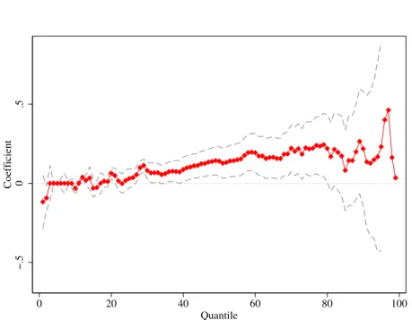
Following Bitler, Gelbach and Hoynes (2006), to get a clearer picture of the effects across the entire risk score distribution, we estimate quantile regressions for the first through 99th quantiles, and plot the resulting coefficients in Figure 2. As predicted (because of the greater variance at higher risk scores), the estimate is generally increasing with the risk score. But it falls close to zero right before the 99th quantile, consistent with outliers being substantially underpriced by the formula, though of course precision is more limited at the highest percentiles.
Given that average Medicare spending of those switching to MA relative to those remaining in FFS does not change after 2003 while their risk scores rise, intensive-margin selection must have increased. As expected, col. (7) shows that, relative to the pre-risk-adjustment period, after 2003 individuals switching into MA versus those remaining in FFS have baseline costs over $1,200 less than their risk scores would predict. As with the extensive-margin results, the coefficients of interest are robust to excluding years before 1997 (col. 8) and controlling for pre-trends (col. 9).22
In the final specification, we focus exclusively on the 2004 through 2006 period and use the actual risk scores provided to us by CMS instead of a simulated risk scores. Here the intensive margin results are even stronger and more precisely estimated, demonstrating that those joining MA after the shift to risk adjustment have significantly lower costs than their HCC risk scores would predict. This larger effect is expected, as our simulated risk-scores (though highly correlated to the official risk scores provided to us by CMS) presumably contain some error and lead to attenuation bias. Finally, note that the main effect of MA status in the intensive-margin regressions is of theoretical interest. The fact that it is close to zero suggests that, among beneficiaries switching to MA in the pre-period, 21As risk adjustment phases in between 2004-2006, we see an increasing trend in the post-period. As such, in col. (6) we estimate pre-period trends and project them forward to the post-period. The coefficient (p-value) on theM A×yearvariable in the pre-period is -.0027 (0.875), suggesting essentially no pre-trends.
22Like the extensive-margin analysis, M A×year trends in the pre-period are essentially zero: a coefficient of−20.69 with ap-value of 0.925.
the HCC risk score successfully predicts costs. This result supports the model’s prediction that risk adjustmentwould have reduced selection had the population of individuals joining MA not changed in response to the policy.
D. Discussion and further verification
One drawback of our identification strategy is that, because we need to calculate risk-scores in the pre-period, we focus on individuals who are in FFS in a baseline year and identify our coefficients off of those who switch the next year from FFS to MA.23 As noted earlier, CMS provided us with actual risk scores for
all individuals in the MCBS from 2004 to 2006. While we cannot replicate the specification in Table 4, we can determine whether—consistent with our findings for MA switchers—risk scores among all MA enrollees are growing faster than those in FFS during this period. We find that in the CMS administrative data, the average MA risk score increased by 12 percent from 2004 to 2006, versus just 1 percent for those in FFS. As such, our estimates above comparing FFS-to-MA “switchers” versus FFS “stayers” closely correspond to comparisons using the
stock of individuals in MA versus FFS.
In Table 5, we move beyond the MCBS to verify our finding of no overall cost differences between FFS and MA enrollees after risk adjustment, as we found in col. (1) of Table 4. We gathered over 8,000,000 hospital discharge records from the twelve states between 2000 and 2006 that require hospitals to record FFS/MA status. Because these states are populous, they represent 42 percent of Medicare beneficiaries during this period. In col. (2) of Table 5, the average MA patient had $1,500 less in charges than his FFS counterpart before 2004— consistent with positive selection in the pre-period—with only $85 (p=.835) of this difference being made up in the post-period—consistent with our results that risk adjustment did not lead MA plans to enroll higher-cost individuals. Interestingly, when we do our best to replicate this regression with the MCBS switcher-analysis by using only annual Part A charges in 2000 to 2006, we find very similar point-estimates (col. 3).
Finally, we follow Batata (2004) and use county-level data to estimate changes in MA selection. She shows that regressing county-level changes in average FFS spending on the change in county-level MA penetration yields a measure of the difference in costs between themarginal person switching between MA and FFS and the FFS stock. While slightly different than our switcher regressions—which compare theaverage person switching from FFS to MA with the average person staying in FFS—one would expect these two selection measures to move in the same direction. As the final column of Table 5 shows, this difference is negative before risk adjustment, reflecting the fact that those on the margin of switch-23In the same report that we cited in footnote 13, MedPAC also examined MA-to-FFS switchers from 2007-2008, whereas this group is too small in the MCBS for us to examine. Consistent with our model, they find that MA enrollees who switch back to FFS areexpensive for their risk score, the parallel result to finding that FFS-to-MA switchers arecheap for their risk score.
ing between MA and FFS have lower costs than those in FFS. Consistent with the switcher analysis and the rest of the table, selection along this margin does not change after risk adjustment (in fact, the point estimate suggests increased selection), though our precision here is somewhat limited.
In summary, our evidence from several datasets indicates that, with respect to actual health costs, those in MA are as positively selected after risk adjustment as before.
V. Did risk adjustment decrease differential selection?
One might assess risk adjustment by estimating how an individual’s annual To-tal Medicare expenditure changes when he switches from FFS to MA, and then compare this change before and after risk adjustment. Total Medicare expen-diture is the total annual cost to Medicare for covering an individual, whether from claims (for FFS enrollees) or capitation payments (for MA enrollees). Un-der perfect risk adjustment (i.e., capitation payments equal to an individual’s expected FFS costs ) whether an enrollee switches between FFS and MA should in expectation have no effect on this variable.
This approach has important limitations. First, comparing the government’s costs as individuals switch between MA and FFS obviously requires focusing only on “switchers,” and thus only a subsample of the data. Yet our model tells us that risk adjustment will decrease overpayments on thestock of those who joined MA before risk adjustment, while having ambiguous effects on those who join after, meaning that looking only at post-period “switchers” could mask the ability of risk adjustment to decrease overpayments. On the other hand, using risk scores only from those who were in FFS the previous year ignores “intensive coding” (as risk scores that first year are based on FFS claims), a serious drawback of risk adjustment that a “switcher” analysis cannot measure.
Second, after 2003, the MCBS does not provide individual capitation payments. In principle, one can recreate them by multiplying the simulated HCC risk scores by county-level benchmarks. However, recall that county benchmarks grow more rapidly post risk adjustment and plans also receive additional “budget-neutrality” adjustments to ease the transition to risk adjustment. As such, one must take a stand on the counterfactual evolution of benchmark payments to isolate the effects of risk adjustment from these coincident payment increases.
In Appendix B, we make assumptions about how each of these missing pieces affects our calculation and conclude that overpayments do not fall post-risk ad-justment. We in fact find a small positive effect—a significant increase in over-payments among those who enroll in MA post-2003 of between $1,500 and $2,000, somewhat but not fully offset by a $700 decrease in overpayments among the still larger population MA “incumbents” who had first joined before 2004–though given the above concerns large error bands must be assumed. Note also that this blended effect should become more positive over time as the incumbents comprise a shrinking share of the MA population given its substantial flux.
In the rest of the section, we focus on a specification that allows us to exam-ine the change in differential selection for all MA and FFS enrollees—not just switchers—before and after risk adjustment, in a manner independent of changes in underlying benchmarks. Specifically, we use mortality as a proxy for costs— which, unlike costs, is both recorded for everyone in the MCBS and independent of how the government changes benchmarks—and regress it on MA status and the risk score. A negative coefficient on the MA variable indicates that, even condi-tional on the risk score, MA enrollees are positively selected. We compare whether this selection conditional-on-the-risk-score is greater in the pre-period (using the demographic risk score) or the post-period (using the HCC risk score).24
Below, we show that our demographic and HCC scores predict the correct amount of variance in the FFS data; that mortality is indeed an excellent proxy for costs in FFS data; and then proceed to the main empirical test.
A. Empirical results
Initial steps. As noted in Section I, the demographic risk score was shown by CMS to account for one percent of FFS cost variance. Col. (1) of Appendix Table 4 shows that the demographic risk scores we calculate account for 1.23 percent of cost variance, using pre-period FFS data. Similarly, CMS calculated that the HCC score accounts for 11 percent of pre-period FFS cost variance. Indeed, in col. (2) ourR2 value using MCBS FFS data is also 11.0 percent. Col. (3) regresses annual costs on whether an MCBS respondent died in a given year. TheR2 value is 15.1 percent, showing that death is in fact a stronger predictor of FFS costs than the HCC risk score itself.
Comparing selection before and after risk adjustment. The first three
columns of Table 6 show that—unconditional on the risk score—those in MA are very positively selected with respect to mortality. They are 1.4 percentage points (more than 25 percent) less likely to die in a given year, relative to their FFS counterparts, which holds relatively constant before and after risk adjustment (cols. 2 and 3). The nearly identical mortality advantage of those in MA pre- and post-risk adjustment adds to the evidence shown in Table 5 that the differences in overall, unconditional health status between MA and FFS enrollees do not change after risk adjustment.
To test risk adjustment, however, we compare conditional differences. In the pre-period, the demographic risk score was more effective in reducing this positive selection—the MA coefficient, while still negative and significant, falls in magni-tude by roughly 75 percent in col. (4) relative to col. (2). In the post-period, conditioning on the HCC risk score in col. (5) only modestly reduces the positive selection into MA—the coefficient on the MA variable falls by less than thirty percent and remains highly significant.
24From CMS, we have HCC risk scores for everyone (both switchers and stayers) in the post-period, and the demographic risk scores can be easily calculated with the background information collected by the MCBS and does not require claims data.
In col. (6), we combine the regressions in cols. (4) and (5) so that we can more easily compare the M A coefficients in the pre- and post-periods. Indeed, the coefficient on MA in the post-period is significantly “more negative” than that in the pre-period, suggesting thatconditional on the risk score that MA plans faced at the time, being in MA indicates a lower conditional probability of dying and thus more positive selection. The final columns shows that this relationship holds when we compare the post-period to a shorter pre-period.
B. Discussion
We can translate these effects into overpayments by using the estimated effect of mortality on total annual Medicare costs. This exercise yields an increase in overpayments of $317. An advantage of the mortality analysis is that it pro-vides an estimate of differential payments independent of the extra statutory overpayments MA plans received, but as a policy matter, MA plans did indeed enjoy higher statutory overpayments in the post-period. Including them yields total overpayment increases between $736 and $988, the smaller estimate equal to roughly nine percent of average per capita FFS annual spending.25
VI. How does selection into MA plans take place?
A. Why are low-cost individuals more likely to be in MA plans?
The evidence in Section IV shows that MA plans enrolled lower-cost individuals both before and after risk adjustment. But how do such patterns emerge when plans must offer the same plans at the same rate to all Medicare beneficiaries in their geographical area of operation? We first explore whether among all MA enrollees, the healthy ones are more satisfied with their care and less likely to return to FFS. This pattern might arise because plans actively treat healthy enrollees better than sick ones so as to differentially retain the former group, or simply because sick individuals do not like the HMO model of care. Through reputation effects, such a result could feed back into patterns of switching into MA as well. This latter pattern could also be driven by targeted advising, with previous studies finding that advertisements for MA plans target healthy people (Mehrotra et al, 2006; KFF, 2008).
25The monthly increase in costs the year an individual dies is $4308 (App. Table 4, col. 3). The increase in conditional selection with respect to mortality after risk adjustment is 0.00613 (Table 6, col. 6), suggesting an increase in overpayments of $4308∗12∗0.00613 = $317 (assuming the relationship between costs and mortality is the same for MA and FFS). The increase in statutory overpayments depends on which pre-period to use as a counter-factual. As noted in Section II, in the three years before the reform, statutory overpayments averaged 103 percent of FFS costs, rising to 108 percent in our post-period. Taking the entire pre-period, where in the early years capitation payments were set to equal 95 percent of per capita FFS costs, we can estimate that capitation payments were roughly 100 percent of FFS costs. Given that per capita FFS costs were $8385 in 2004, the statutory overpayment increases are between 0.05∗$8385 = $419 and 0.08∗$8385 = $671, so, adding the increase in overpayments from differential selection alone gives a total overpayment increase between $736 and $988.
The MCBS asks respondents to rate their satisfaction with their overall health care “last year” as well as specific aspects of it. As the question is asked in the fall, it is difficult to know whether individuals are answering based on their experience so far in the current year or in the previous calendar year. As such and in contrast to our previous analyses, here we focus on those who did not switch (either from FFS to MA or from MA to FFS) the previous year by comparing individuals in MA in both years with those in FFS in both years.
Ideally, we would explore whether satisfaction is higher among MA recipients who are more profitable to insurers. But because we do not have health care cost or claims data for those in MA, we use self-reported health as an admittedly imperfect proxy and investigate whether good health predicts satisfaction with one’s health care in MA more than in FFS:
(3) Satisf actionit=βM Ait×Healthit+γM Ait+Hit+λXi+δt+it, In this specification, Satisf action measures individuals’ reported satisfaction with different aspects of their health care and varies from one (very dissatisfied) to four (very satisfied), Health is a five-category self-reported health variable,
Hare its corresponding fixed effects, and all other notation follows that used in previous equations. The health fixed effects account for the fact that in both MA and FFS, poor health correlates with negative feelings toward one’s health care. Thus the interaction term explores how much more or less sensitive enrollee sat-isfaction is to underlying health in MA versus FFS. We control for demographic characteristics inX because different groups may assess their health and health care differently. If MA plans treat healthier enrollees better, we would expect
β >0.
Table 7 displays the results from estimating equation (3) via OLS. We demean the Health variable in M A×Health, so that the M A main effect represents the association with MA enrollment for someone with mean self-reported health. The first row reports results when overall satisfaction serves as the dependent variable. The MA main effect is negative—suggesting that someone of average health reports lower satisfaction in MA than in FFS. This estimate is surprising given that MA enrollees self-selected into MA and given the large overpayments to MA plans, which could lead to additional benefits. But then again MA enrollees may simply be harder to please.
We instead focus on the coefficient on the interaction term, which is positive and significant, indicating that good health predicts satisfaction with MA plans more than it does satisfaction with FFS. In fact, only among those who report being in “excellent” health do MA plans receive a higher rating than FFS (not shown). Moreover, relative to FFS enrollees, MA enrollees exhibit a more positive gradient of satisfaction with respect to health in all nine categories surveyed by the MCBS, and for a majority of categories this difference is statistically significant.
The last row of Table 7 investigates whether sicker MA enrollees “vote with their feet” and exit at higher rates than do sicker enrollees in FFS. Instead of sat-isfaction ratings, we regress whether an individual changes his coverage status—to
MA if he is currently in FFS, to FFS if he is in MA—on the same set of explana-tory variables.26 Indeed, the same pattern emerges—not only are MA enrollees less likely to retain their current coverage status in general, but this difference is especially pronounced for those in self-reported poor health. As such, among MA patients, the sickest are the most likely to return to FFS each year.
B. Possible mechanisms underlying the changes after risk adjustment
The results in Table 7 provide an explanation for why higher-cost enrollees tend to be in FFS, but they do not explain how individuals with low costs relative to their risk score found their way into MA plans after risk adjustment. While we cannot provide a definitive answer given the available data, we believe several factors are at work. First, insurers have a wealth of data, both on their own MA enrollees and from their operations in the non-Medicare market. In fact, because insurers (unlike CMS) have data on the medical claims and costs of MA benefi-ciaries, along this dimension plans have more information than the government. Second, CMS does not adjust for factors such as race, ethnicity, and income, which are not only related to health costs but, through targeted advertising, are also relatively easy for MA plans to select on. Given that the variance in costs grows with the risk score, demographic differences that are small on average could be very large for groups with high risk scores or for a specific disease category. Plans have the data to determine that, for example, Hispanics with heart disease are $3,500 cheaper than their risk score would suggest and then target advertising accordingly. If demographic or other observable factors explain how costs vary from the risk score’s prediction within a disease category, then plans may have the ability to differentially enroll people who are low cost for their risk score.27
We explore empirically whether after risk adjustment MA plans appear to en-gage in selection along profitable Disease×Demographic Group margins. We start with a specific example. Consider HCC10, “Breast, Prostate, and Colorectal Cancer,” which, unlike the other major categories (the ten most common of which are listed in Appendix Table 1) combines multiple diseases. Given the prevalence rates of these diseases, the large majority of women (men) in this category will have breast (prostate) cancer. Moreover, past medical research (Yabroff et al., 2008) has shown the annual cost of breast cancer treatment to be roughly $1,900 cheaper than that of prostate cancer even after accounting for demographic differ-ences between the two groups.28 Therefore, we have a common disease group in which we can identify a large subgroup of individuals (women) who were under-priced before risk adjustment and are over-under-priced after. While all individuals in 26For this analysis, we expand our MCBS sample to include individuals who switch from FFS to MA (or vice-versa) in each year.
27See recent work by Kim and Aizawa (2013) using advertising spending by MA plans to document that such spending is higher in localities where the cost differences between the sick and healthy are largest and thus the benefits of risk-selection are greatest.
28In our data, the gender difference in costs among those with HCC 10 is roughly $1,200, likely because of attenuation bias from colorectal cancer.
Category 10 were less likely than other Medicare beneficiaries to join MA in the pre-period, women—but not men—in this category are more likely to join after risk adjustment (p < .02).
Next, we explore whether, more generally, MA enrollment in the post-period ap-pears to correspond toDisease Category×Gender“errors” in the risk-adjustment formula. Because of power constraints, we consider only the largest ten disease categories and use gender because other categories create unequal splits of dis-ease groups and thus very small cells. While HCC10 provides an especially nice example given that two diseases are combined, it is also the case that men and women appear to differ systematically in the costs they incur for the other nine disease groups. For each of the twenty cells, we estimate the “error” in the risk-adjustment formula using pre-period FFS data and pre-period benchmarks.29 As Appendix Figure 3.A shows, while the errors are roughly centered on zero, there exists substantial variance. On the y-axis, we plot the probability an individual in each cell switches from FFS to MA in the post-period. Indeed, there is a positive correlation between overpayment errors and the post-period FFS-to-MA transi-tion probability. Appendix Figure 3.B shows that, by contrast, there is no such correlation between the payment errors and pre-period transition probability—we would expect none, since risk adjustment did not exist in this period and thus risk-adjustment errors would be meaningless to plans.
These results provide additional evidence that insurers responded to the policy-induced change in financial incentives by enrolling those Medicare recipients whose profitability increased most after the shift to risk adjustment.
VII. Welfare and Policy Implications
While we have provided evidence suggesting that risk adjustment did not ac-complish its goal of reducing the government’s overpayments, a full welfare anal-ysis would include the effects on producer and consumer surplus. While the evidence presented in this section is hardly definitive, it begins to shed light on the policy’s wider implications.
A. The effect of risk adjustment on plan profits
We do not have access to actual MA-specific profit data from insurers, a lim-itation that appears to be shared by all papers in the MA literature. However, our model does speak directly to plan profits—after risk adjustment, profits fall (even if overpayments rise) because screening costs increase. Note also this pre-diction refers to “payment-neutral” risk adjustment—which, recall, was our term for a risk-adjustment model in which, essentially, the government is not trying to systematically under- or overpay plans on average.
29To capture as closely as possible the errors MA plans would encounter, we use data from 1997 to 2002, as the risk-adjustment formula was calibrated using 1999-2000 FFS data and we add two years on either side to gain precision.
While we do not have actual profit data to verify the model’s prediction, ev-idence from plans’ reactions to risk adjustment suggest they believed payment-neutral risk adjustment would hurt their profits. The implementation of the mild precursor to the HCC model (which, recall, explained 1.5 percent of cost varia-tion) was explicitly payment-neutral. Many private insurers formally called on CMS—which tacitly agreed the reform would hurt plans—to delay the imple-mentation of risk adjustment or to provide extra “budget-neutrality” payments to compensate for risk adjustment.30 Indeed, perhaps to avoid a similar backlash, as we explain in Sections I and II, CMS increased the risk-adjusted capitation pay-ments by roughly ten percent as the HCC risk-adjustment formula was phased in. Thus, when risk adjustment is not augmented with additional payments, both CMS and the private insurers expected profits to fall, consistent with our model’s predictions.
In our model, risk adjustment can increase government spending while decreas-ing plan profits because it increases insurers’ screendecreas-ing costs. The model assumes that strategies that allow insurers to find, for example, the cheapest diabetics (an optimal strategy after risk adjustment) are costlier on a per-enrollee basis than avoiding diabetics altogether (optimal before risk adjustment). This extra money could be spent in ways that increase consumer welfare, like improving the quality of medical care, or in ways that likely do not, such as engaging in targeted advertising or devising complicated screening strategies. Ultimately, the extent to which this extra spending benefits consumers is an empirical question.
B. The effect of risk adjustment on consumer welfare
In this subsection, we explore whether risk adjustment improved consumer wel-fare along a variety of observable dimensions. To conserve space we only briefly describe the data and estimating equations and refer readers to the Appendix for greater detail. It is worth emphasizing here that, through the accelerated growth of county benchmarks and “budget neutrality” payments, MA plans received in-creases in capitation payments in the post-period beyond those that we attribute to their endogenous reaction to risk adjustment. As such, if some of these over-payments were passed on to MA enrollees after 2003, our estimates serve as an upper bound for benefits to consumers from risk adjustment alone.
Comparing MA v. FFS before and after risk adjustment. We begin by
examining the simple question of whether MA enrollees report higher satisfaction after risk adjustment. We regress each of our satisfaction measures on M A×
Af ter 2003, its lower-order terms and the controls in Table 7. As shown in Appendix Table 5, the coefficient onM A×Af ter 2003 is negative for five and positive for four, though rarely statistically significant, suggesting that post-risk-adjustment, MA enrollees do not report relative increases in their satisfaction.
30See http://www.cms.gov/MedicareAdvtgSpecRateStats/Downloads/Announcement2000.pdf This same document shows that the PIP-DCG model was meant to be explicitly payment neutral.
We probe further on these results by controlling for differential trends among MA recipients prior to the shift to risk adjustment (panel B). In contrast to our previous results for extensive and intensive margin selection, which were unaf-fected by the inclusion of these trends, here the point estimates generally increase and suggest that MA recipients experienced an increase in satisfaction following the shift to risk adjustment. The increase in the estimated impacts is driven by a negative trend in satisfaction with MA prior to 2004, which is somewhat arrested after 2003. However, in the post-period, MA recipients still report lower satis-faction in eight of the nine categories the MCBS collects (not shown). As such, while there might be some improvement relative to trend, it is not large enough to close the MA-FFS satisfaction gap despite the increase in payments to MA plans in the post-period.
Nor did the positiveM A×Healthsatisfaction gradient documented in Table 7 shift post-risk-adjustment, as one would have predicted had MA plans began to cater to those in worse health. In Appendix Table 6 we interact M A×Health
with a post-risk-adjustment indicator variable, and the only significant effect is a further positive tilt in one category and no statistically significant effect on the others.
Did risk adjustment improve the Medicare program more broadly?
To fully assess risk adjustment we need to consider its effects on the entire Medi-care program. Suppose, for example, that risk adjustment allowed for better sorting of beneficiaries between MA and FFS, and thus everyone was better off. The above analysis would obscure such an effect by not considering the benefits to FFS enrollees as well. Moreover, because the types of people switching from FFS to MA change after 2003 (they have higher risk scores, e.g.), the analysis above—comparing MA versus FFS enrollees after 2003—could be contaminated by compositional changes. We thus perform a number of analyses not subject to these critiques.
As envisioned by policy-makers, risk adjustment would increase insurers’ incen-tives to expand health care options for those in poor health. As such, one would expect those in poor health to be relatively more satisfied with their health care options post-risk adjustment. We thus estimate our various satisfaction measures as a function of Health×Af ter 2003, its lower-order terms, and the controls included in Table 7. As shown in Appendix Table 7, the coefficient on the inter-action term is positive for all nine categories and more often than not significant, meaning that after risk adjustment those in poor health are relativelylesssatisfied with their health care.
This result is central to the welfare effects of risk adjustment because the gra-dient of satisfaction with respect to health status speaks to the insurance value of Medicare. Put differently, a system in which healthy people receive the high-est quality health care would not seem to allocate resources from the “good” to the “bad” state, as consumption-smoothing requires. The positive coefficients on