A statistical approach to virtual cellular experiments: improved causal discovery using accumulation IDA (aIDA)

(1)

Systems biology

A statistical approach to virtual cellular

experiments: improved causal discovery

using accumulation IDA (aIDA)

Franziska Taruttis*, Rainer Spang and Julia C. Engelmann*

Department of Statistical Bioinformatics, University of Regensburg, 93053 Regensburg, Germany

*To whom correspondence should be addressed.

Associate Editor: Igor Jurisica

Received on March 31, 2015; revised on July 9, 2015; accepted on August 1, 2015

Abstract

Motivation:

We address the following question: Does inhibition of the expression of a gene X in a

cellular assay affect the expression of another gene Y? Rather than inhibiting gene X

experimen-tally, we aim at answering this question computationally using as the only input observational

gene expression data. Recently, a new statistical algorithm called Intervention calculus when the

Directed acyclic graph is Absent (IDA), has been proposed for this problem. For several biological

systems, IDA has been shown to outcompete regression-based methods with respect to the

num-ber of true positives versus the numnum-ber of false positives for the top 5000 predicted effects. Further

improvements in the performance of IDA have been realized by stability selection, a resampling

method wrapped around IDA that enhances the discovery of true causal effects. Nevertheless, the

rate of false positive and false negative predictions is still unsatisfactorily high.

Results:

We introduce a new resampling approach for causal discovery called accumulation IDA

(aIDA). We show that aIDA improves the performance of causal discoveries compared to existing

variants of IDA on both simulated and real yeast data. The higher reliability of top causal effect

pre-dictions achieved by aIDA promises to increase the rate of success of wet lab intervention

experi-ments for functional studies.

Availability and implementation:

R code for aIDA is available in the

Supplementary material

.

Contact:

[email protected], [email protected]

Supplementary information:

Supplementary data

are available at

Bioinformatics

online.

1 Introduction

Understanding of the complex molecular networks underlying cellular processes is the key challenge of systems biology. Here, we focus on gene regulatory networks. Interpreting these networks causally re-quires a direction of information flow. Given a causal network, the most basic question is: If I perturb gene X, what happens to gene Y? Of course, this question can be answered experimentally by inhibiting X, e.g. by PCR-based gene deletion strategy (Baudin et al., 1993; Wach, 1996), RNA interference (Fire et al., 1998), or CRISPRi (Larsonet al., 2013) screening, and observing Y. We here discuss to what extend the same question may be answered in a virtual way, i.e. without the need to perform a cellular perturbation experiment.

A high-throughput version of this problem would be the following: Find all pairs of genesðX!YÞ, where perturbingXaffectsY.We refer to this causal data mining approach as causal discovery.

Statistically, the challenge is to estimate causal effects between random variables from purely observational data. For gene expres-sion data the causal effect of gene X on gene Y can be defined as the number of units gene Y changes in expression, if the expression of gene X is experimentally altered by one unit. Causal Networks are a well established statistical framework for analyzing this problem (Pearl, 2000).

In causal transcriptional networks the nodes of a directed acyclic graph (DAG) are random variables representing genes and their

VC_{The Author 2015. Published by Oxford University Press.} 1

This is an Open Access article distributed under the terms of the Creative Commons Attribution Non-Commercial License (http://creativecommons.org/licenses/by-nc/4.0/), which permits non-commercial re-use, distribution, and reproduction in any medium, provided the original work is properly cited. For commercial re-use, please contact [email protected]

Bioinformatics, 2015, 1–8 doi: 10.1093/bioinformatics/btv461 Advance Access Publication Date: 6 August 2015 Original Paper

at Universitaetsbibliothek Regensburg on November 17, 2015

http://bioinformatics.oxfordjournals.org/

(2)

expression values. A directed edge from X to Y denotes that the ex-pression of X causally and directly influences the exex-pression of Y. Consequently, the expression of Y is determined by the expression of its parents in the network. If the causal network is known, Pearl’s do-calculus allows estimating the strength of the causal effects be-tween pairs of random variables from observational data (Goldszmidt and Pearl, 1992;Pearl, 1995). However, causal tran-scriptional networks are largely unknown. Multiple statistical algo-rithms have been established to estimate the undirected skeleton of a network from conditional independence tests (Huynh-Thu et al., 2010; Margolin et al., 2006). The PC algorithm (Kalisch and Bu¨hlmann, 2007;Spirteset al., 2000) allows to define the direction of some edges allowing for a causal interpretation of the network. The network cannot be fully directed because different networks with identical skeletons can encode the same conditional independ-ence assumptions and thus can not be distinguished on observational data only (Verma and Pearl, 1991).

Recently,Maathuiset al.(2009)introduced the Intervention cal-culus when the Directed acyclic graph is Absent (IDA) algorithm, which combines partial estimation of the network with the estima-tion of lower bounds for causal effects between genes. They prove consistency of the bounds (Maathuiset al., 2009) and show in appli-cations that IDA outperforms regression-based methods in terms of number of true positives versus number of false positives for the top 5000 predicted effects on the transcriptome of yeast gene deletion strains from a large dataset of expression profiles of wild type yeast (Maathuiset al., 2010). However, in simulations with large net-works and medium sized datasets, which are typical for many biolo-gical applications, networks often cannot be reconstructed correctly. Stekhoven et al. (2012) suggest using stability selection (Meinshausen and Bu¨hlmann, 2010), a subsampling strategy that is wrapped around IDA as a remedy. In fact, their CStaR algorithm outperforms plain IDA with respect to true positive selections versus false positive selections (Stekhovenet al., 2012).

Here we propose an alternative subsampling strategy in combin-ation with a modificcombin-ation of the IDA algorithm called accumulcombin-ation IDA (aIDA). Our method represents an improvement over CStaR, IDA, and regression based methods as demonstrated for both simu-lated and two yeast datasets.

2 Causal discovery

2.1 Causal transcriptional networks

We represent transcriptional causal networks by DAGs consisting of nodesX¼X1; :::;Xpand edgesE¼E1; :::;Es. Every gene is repre-sented by one node in the network. Statistically, every node is a ran-dom variable whose values indicate the expression levels of a gene. We further assume that the variables follow a multivariate Gaussian distribution. Edges represent conditional dependencies; nodes that are not connected represent variables that are conditionally inde-pendent. Moreover, we interpret the edges causally. If there is a dir-ected edgeX!Y, we assume that an experimental perturbation of the expression level ofXwill affectY, but not vice versa. A DAG fully specifies the conditional dependencies of all nodes (Pearl, 1988), but not vice versa. Several DAGs with the same skeleton of undirected edges and the same v-structures (Pearl, 2000) encode the same conditional dependency structure (Verma and Pearl, 1991). These equivalence classes of DAGs can be represented by completed partially directed acyclic graphs (CPDAGs) that consist of the joint skeleton and the directed edges which are common to all DAGs in the equivalence class (Chickering, 2002).

2.2 Causal effects

In a hypothetical perturbation experiment we may increase the random variableXby one unit (X7!Xþ1) and observe the effect on a second variableY.IfYis changed byY7!Yþb, we callbthe causal effect of XonY.Given a causal network and a dataset of joint observations of the nodesX, Pearl’s do-calculus (Goldszmidt and Pearl, 1992;Pearl, 1995) provides guidelines how to estimate causal effectsbfor all pairs of nodes. In the Gaussian case one can use a linear regression ofYon Xand a set of additional nodesZthat fulfill the Back-door criterion (Pearl, 2000), a criterion that only depends on the topology of the underlying causal network. A set of variablesZsatisfies the Back-door criterion relative to an ordered pair (X,Y) in a DAG G, if

i. no node inZis a descendant ofX.

ii. Zblocks (seeSupplementary Section 1) every path betweenX andYthat contains an arrow intoX

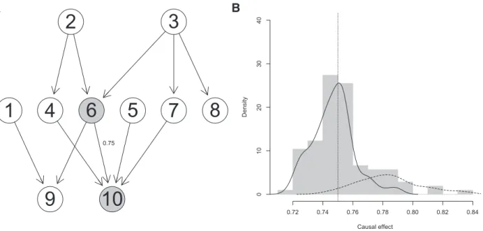
(Pearl, 2000). It can be shown, that the true parents of a nodeXdo always fulfill the Back-door criterion relative to every ordered pair (X,Y) (Pearl, 2000). InFigure 1A the set of nodes {2,3} fulfills the Back-door criterion relative to the ordered pair (6,10). In addition, the set {4,7} fulfills the Back-door criterion relative to the ordered pair (6,10), while for example the set {4} does not fulfill the Back-door criterion, because the path (6,3,7,10) remains unblocked.

LetZ¼ ðZ1;. . .;ZkÞbe a set of nodes fulfilling the Back-door criterion, and letb¼b0;bX;bZ1;. . .;bZjbe the least squares fit of the linear regression

Y¼b0þbXXþ X

i

bZiZiþ; (1) thenbXis a consistent estimator of the causal effect of X on Y

(Maathuiset al., 2009).Zadjusts the regression for possible con-founders that affectXandYsimultaneously, thus creating spurious correlations betweenXandY.An example for an adjustment setZ that satisfies the Back-door criterion of a nodeXwith respect to all other nodesYis the set of true parents ofX.

2.3 IDA and CStaR

For transcriptional networks the underlying causal graph is mostly unknown and needs to be estimated. An obvious idea is to first re-construct a causal network and then estimate causal effects thereof usingEquation (1). Several algorithms have been proposed to esti-mate the equivalence class of a DAG from observational data (Chickering, 2002,1996;Dash and Druzdzel, 1999;Madiganet al., 1996;Meek, 1995;Pearl, 2000). IDA uses the PC-algorithm (Spirtes

et al., 2000), which estimates the CPDAG in a two-step procedure. In the first step, the skeleton and the v-structures of the CPDAG are estimated by testing for conditional independence. In the second step, orientation rules are applied (Meek, 1995), which exploit the facts that (i) the network cannot be cyclic, and (ii) that no new v-structures are found in an equivalence class. A parameterais used to calibrate the sparseness of the estimated network. Large values of a increase the number of edges within a network. Importantly, increasingaalso increases the runtime of the algorithm significantly, such that one often needs to compromise on the sparsity of the net-work to keep computations feasible.

The existence of equivalent DAGs complicates the estimation of causal effects.Maathuiset al.(2009)have demonstrated that it is still feasible to derive lower bounds of causal effects using their IDA algorithm. In a computationally elegant and efficient way, IDA enu-merates all possible parent sets of a nodeXin a CPDAG, and calcu-lates causal effects ofXon all its descendants using any one of the

(3)

parent sets as adjustment setsZinEquation (1). This yields a set of estimated effects, and its minimum is used as a lower bound. IDA is asymptotically consistent.

From the systems biology perspective, IDA was ground-break-ing, becauseMaathuiset al.(2010)succeeded in predicting expres-sion changes of 5361 genes in 234 yeast deletion strains from 63 expression profiles of wild type yeast, thus constituting the first high throughput analysis of virtual perturbation experiments.

Transcriptional networks consist of tens of thousands of genes. Typically, however, one has not more than at best a few hundred observations of their gene expression values. In situations with many nodes and few observations the accuracy of estimated CPDAGs by the PC algorithm is poor (Kalisch and Bu¨hlmann, 2007). As a remedyStekhovenet al.(2012)suggest applying stabil-ity selection (Meinshausen and Bu¨hlmann, 2010) on the IDA algo-rithm. Ksubsets of samples are drawn and sets of causal effect bounds are estimated for all of them using IDA. Finally, genes are ranked by how often they appear in the topqgenes with the highest effects. This procedure is repeated for several values ofqand the me-dian rank is used to calculate the final rank of a gene. This modified IDA algorithm called CStaR was demonstrated to improve on causal discovery (Stekhovenet al., 2012).

2.4 Limitations

A limiting factor in both IDA and CStaR is the poor accuracy of the estimated CPDAGs and the strong dependence of subsequent steps on a valid causal network (Supplementary Figs S1andS2). Albeit it is difficult to improve on the quality of estimated networks, we argue that there is a more effective way to extract causal informa-tion from imperfect networks. More specifically, we have identified two steps in the IDA/CStaR procedure that confine causal discovery. 2.4.1 Selecting a causal effect from a multiset

For a given pair of nodesXandYand a given CPDAG, IDA calcu-lates multiple causal effects ofXonY, if the CPDAG connectsXto other nodes via undirected edges. Both IDA and CStaR are

conservative in that they report the minimum of the effect set. While the minimum is a valid lower bound of the causal effect, it represents a biased estimate that can lead to missed causal discoveries. 2.4.2. Summarizing effects across subsampling runs

CStaR applies stability selection to detect stable causal effects. It prefers gene pairs that repeatedly obtain a high score. The focus on gene pairs with the highest scores can lead to missed causal effects with smaller effect sizes.

Whether an estimated effect in the set of causal effects from X on Y associated with a CPDAG,MðX!YÞ, is valid or not depends on the corresponding adjustment setZused inEquation (1). IDA and CStaR aim at deriving valid effects by identifying the true par-ents of the nodeX.If the CPDAG is correct, at least one of the ef-fects inMðX!YÞis based on the true parents ofXand thus valid, but we do not know which one it is. If the CPDAG is incorrect, it is well possible that all values inMðX!YÞare invalid.

3 The aIDA algorithm

3.1 Motivation

We aim at distinguishing between valid and invalid effects both within multisets of effects and across subsampling runs. If the causal network is known, the Back-door criterion and other graph-based criteria (Tian and Pearl, 2002) can be used. If the network is not known, we argue that the distribution of effects across subsampling runs is helpful to estimate the true causal effect. We use estimated causal effects from simulated data using known causal networks to study features of the estimated CPDAGs and the distributions of valid causal effects versus invalid causal effects.

3.1.1 Estimated parent nodes often yield valid estimates even if they are not the true parents

If the network underlying a dataset is estimated correctly, we can es-timate valid causal effects from it. But absolutely correct networks

1

2

3

4

6

5

7

8

9

10

0.75

B

A

Causal effect Density 0.72 0.74 0.76 0.78 0.80 0.82 0.84 0 1 02 03 04 0

Fig. 1.Example for accumulation of the causal effect for a small simulated dataset. (A) Causal network. The causal effect of interest is the one of node 6 on node 10 (gray nodes). The true causal effect is 0.75. (B) Histogram over all estimated causal effects and the density for the effects that fulfill (solid line) or do not fulfill (dashed line) the Back-door criterion. Causal effects estimated using estimated adjustment sets which do not fulfill the Back-door criterion (dashed line) do not co-incide with to the true causal effect, while the causal effects estimated using valid adjustment sets agree with the causal effect (vertical line)

(4)

are no strict requirement to calculate causal effects. Certain benign mistakes do not impede causal effect estimation. If the estimated parents fulfill the Back-door criterion they yield valid estimates even if they are not true parents. For a given DAG with edge weights that represent direct causal effect strengths we can generate artificial gene expression data (Details are given in the Supplementary Materials Section 3.1). We generated 50 samples for a random DAG of 1000 nodes, drew 100 subsamples of sizen¼25, and ran the PC-algorithm as implemented in (Colombo and Maathuis, 2012) on each subsample, resulting in 100 CPDAGs. From all pairs of nodes

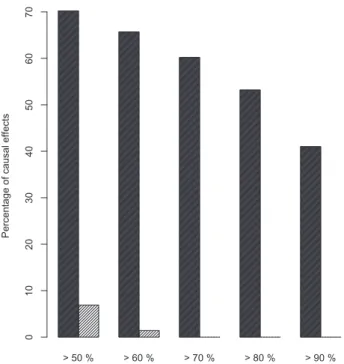
ðX!YÞwe calculated the multisets of possible estimated parents of X.Since we know the correct parents ofXin the simulation scen-ario, we can count how often the PC-algorithm correctly identifies a parent set. In these cases IDA can derive valid causal effects. However, finding the correct parent sets is a sufficient but not a ne-cessary criterion to get valid estimates. In fact, every gene setZthat fulfills Pearl’s Back-door criterion also yields valid causal effect esti-mates. In our simulations from known networks (seeSupplementary Materialfor details on data simulation), we can verify whether an estimated parent set fulfills this criterion and count how often this is the case.Figure 2shows that although estimated parent sets often are not the true parents, they nevertheless frequently fulfill the Back-door criterion and will hence generate valid estimates of causal ef-fects. In other words, finding the true parents is difficult, whereas obtaining a set of estimated parents satisfying the Back-door criter-ion is not. For example, in more than 40% of the cause-effects pairs

the Back-door criterion was fulfilled in more than 90% of the esti-mated parent sets over the 100 subsampling runs, conversely there were no subsampling runs that contained at least 90% true causal parent sets. Similar observations can be made when reconstructing real biological networks (Supplementary Fig. S3). This explains in part why IDA and CStaR are successful in spite of the poor perform-ance of the PC-algorithm.

3.1.2 Valid effects generate peaks in the effect histograms

We next usedEquation (1)to estimate causal effect sets for all pairs of nodesðX!YÞand all estimated parent sets that can be derived from the CPDAGs. We pool these numbers both across effect multi-sets and subsampling runs and visualize their distribution in the light gray histogram ofFigure 1B.

The solid curve inFigure 1B is a smoothed density estimate of all effects from node 6 on node 10 across 100 subsampling runs derived from valid adjustment sets. We observe a pronounced peak in this density around the true causal effect (dotted vertical line). This is be-cause estimates derived from valid adjustment setsZare unbiased estimates of the true causal effect and, hence, scatter around it. The true parents of the cause are always a valid adjustment set, but they are not necessarily the only one. Valid are all sets that fulfill the Back-door criterion relative to the cause and the effect of interest. The dashed curve shows the density of the estimates that are not derived from valid adjustment sets. This distribution is not centered around the true effect. Estimates based on invalid adjustment sets can take any value, and their corresponding distribution is un-known. Since the Back-door criterion is not a necessary condition forZto be a valid adjustment set, some of these estimates might still be valid but others are not.

If a large fraction of effects is valid, one would expect them to have similar values centered around the true causal effect, and there-fore give rise to a peak in the histogram.

This observation is the motivation for the algorithm described below. The basic idea is to pool effects across multisets and subsam-pling runs and to use the mode of the smoothed histogram as causal effect estimate.

3.2 Algorithm

The input of our algorithm is a set of expression profiles consisting ofpgenes observed innsamples. This data is observational, i.e. the cells were not perturbed. We assume that all samples were drawn from the same underlying joint distribution of gene expression levels. The output of our algorithm is an ordered list of triples (X,Y,C), wereXandYare genes andCis the estimated causal ef-fect ofXonY.The list is sorted by the absolute value of the effect strengthC.

The algorithm performs the following steps:

1. Randomly drawKsubsets of samples of size l, resulting inK resampled datasets.

2. For each of these subsets estimate a CPDAG using the PC-algo-rithm as implemented in Colombo and Maathuis (2012)with sparseness parametera, resulting inKCPDAGs on the same set of nodes.

3. For every ordered pair of genesðX!YÞextract the multisetsM

ðX!YÞ of possible estimated parents of X and pool them across all CPDAGs.

4. For all elementsZof this multiset estimate a causal effect using the regression model fromEquation (1).

5. Generate one histogram of estimated effects per gene pair (Accumulation step). Smooth these histograms using a Gaussian > 50 % > 60 % > 70 % > 80 % > 90 %

Percentage of subsamples that fulfill the backdoor-criterion

Percentage of causal effects

0 1 02 03 04 05 06 07

Fig. 2.The Back-door criterion is fulfilled frequently even if the PC algorithm rarely detects the true parents. One thousand cause-effect pairs were sampled randomly from a network with 1000 nodes. For each of these pairs we counted how often the Back-door criterion was fulfilled by the estimated parent sets within the 100 subsamples (black bars) and how often the parent set was the true parent set (gray bars). Thex-axis shows the percentage of estimated causal effects of this 100 subsampling runs where the Back-door criterion was fulfilled. They-axis displays the proportion of the 1000 sampled cause-effect pairs for which at least x% of the estimated parent sets from the 100 subsampling runs fulfilled the criterion (black) or were the true parent sets (gray). The detection of true parent sets is a very hard task, but meeting the Back-door criterion is not

(5)

kernel, detect the mode in the smoothed histogram and use it as an estimate for the causal effectCofXonY.

6. Collect all causal effects in appmatrix. Sort the effects by the absolute value ofC, and output this sorted list.

The algorithm follows CStaR in steps 1–4 but differs from CStaR in step 5. Step 6 ranks all gene pairs by effect size to achieve results comparable to CStaR. Since the accumulation idea is added to the IDA concept, we call our algorithm aIDA for accumulation based IDA.

4 Results

aIDA and CStaR (Stekhovenet al., 2012) were applied to both simu-lated datasets and two gene expression microarray datasets from Saccharomyces cerevisiaeusing the order independent implementa-tion of the PC algorithm (Colombo and Maathuis, 2012; Kalisch

et al., 2012). For the simulated datasets true causal effects are known from the simulation process. For the microarray datasets the target set of causal effects is calculated as described inMaathuiset al.(2010)from interventional experiments (single knock-out strains, see details in Section 5.1 of theSupplementary Materials).

4.1 Parameter calibration

aIDA depends on the calibration of several parameters. The most critical of them is the sparseness parameteraof the PC algorithm (Kalisch and Bu¨hlmann, 2007). Since a is shared by aIDA and CStaR, its calibration does not impede a fair comparison of the methods. The other parameters were set to the recommended values from CStaR (seeSupplementary Materials Section 6). For the band-width of the Gaussian kernel we used default values of the density() function from basic R, since further calibration did not improve ef-fect estimation. A largeraleads to denser CPDAGs and larger multi-sets. This in turn leads to more regression parameters that need to

be estimated fromEquation (1), which might increase the standard error of the effect sizebX.We tested the recommended value fora

from the IDA literature but observed for both, the simulated and real data, that resulting CPDAGs can have very different numbers of edges in comparison to previous publications. This is further aggra-vated by a correction of the implementation of the PC algorithm, which leads to systematically sparser graphs for the same values of a, especially for graphs with many variables and few observations (Colombo and Maathuis, 2012).

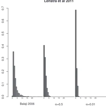
For the simulated datasets we have calibratedasuch that we obtain CPDAGs with densities similar to the expected density (Supplementary Figs S4andS5). The histograms show, thata¼0:5 is a realistic value for a. Additionally, we show that choosing a higher value ofaleads to a better performance (Supplementary Figs S1andS2). For the datasets fromS.cerevisiaewe compared the den-sities to a density derived from a transcriptional regulatory network published byBalajiet al.(2006)(Figs 3and4). We observed that both alpha¼0.01 and alpha¼0.5 underestimate the density of the network. Although the data suggest using an alpha even above 0.5, we did not increase it further due to runtime constraints.

4.2 Performance of aIDA on simulated data

First, we tested the performance of aIDA on simulated datasets gen-erated from known causal Gaussian networks. We simulated ran-dom DAGs of various sizes and augmented their edges with weights sampled from a uniform distribution on the interval (0.1,1). The weights represent direct causal effect strengths. For each DAG, we generated artificial datasets of varying size using the R package pcalg (Kalischet al., 2012). Details on the data generation are given in thesupplements, Section 3.1. We use these data to evaluate the performance of aIDA and compare it to that of CStaR. A compari-son to plain IDA is not needed, because it has already been shown that it is outcompeted by CStaR with respect to true positive selec-tions versus false positive selecselec-tions (Stekhovenet al., 2012). Fig. 3.Comparison of the number of parents of the network fromBalajiet al.

(2006)and the estimated networks using different values ofafor theHughes

et al.(2000)dataset. The distribution of parents estimated from observational

data using the higher value ofais more similar to the true distribution of the number of parents

Fig. 4.Comparison of the number of parents of the network fromBalajiet al.

(2006)and the estimated networks using different values ofafor theLenstra

et al.(2011)dataset. The distribution of parents estimated from observational

data using the higher value ofais more similar to the true distribution of the number of parents

(6)

In a first analysis we randomly simulated two sets of 10 small DAGs with 100 nodes each. For the first set we generated 10 small datasets with each set containingn¼50 samples, and for the second set we simulated 10 large datasets ofn¼1000 samples. We then run aIDA and CStaR on this data, both using 100 subsamples of sizen 2 and a sparseness parameter ofa¼0:1.Figure 5shows barplots of the partial areas under receiver operating characteristics (ROC) curves (pAUC) up to 100 false positives. The error bars correspond to standard errors across the 10 datasets with 50 and 1000 samples, respectively. aIDA outperforms CStaR for both large and small datasets with respect to pAUC up to 100 false positives.

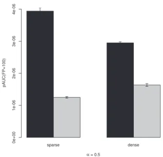
Both CStaR and aIDA become impractically slow for datasets with more than 1000 nodes and realistic settings ofa. In a second analysis we tested aIDA on 5 sparse and 5 dense random networks of size 1000. The sparse and dense random networks contain ap-proximately 1250 and 2500 edges, respectively. We simulated small datasets of 50 samples for each graph. We again used both aIDA and CStaR to rediscover the causal effects in the networks and compared their prediction performances.Figure 6shows bar-plots of the pAUC for the 5 datasets generated from dense and sparse graphs, respectively, up to 100 false positives fora¼0:5 (for more values ofasee Supplementary Figs S1andS2). Again aIDA outperforms CStaR, and achieves its best results for larger settings ofa.

4.3 Application to gene expression data of

S.cerevisiae

deletion strains

aIDA and CStaR were applied to two large scale gene expression studies conducted in yeast. Both datasets analyzedS.cerevisiae sin-gle-gene deletion mutants (Baudinet al., 1993;Wach, 1996). The datasets contain both observational data of wild type yeast and ex-pression data from many individual deletion strains. We ran aIDA and CStaR on the wild type data to predict causal relationships between genes from observational data and validate these predic-tions using the data from the corresponding intervention experiments.

4.3.1 Application to data fromHugheset al. (2000)

Hugheset al.(2000)analyzed 276 deletion mutants and 63 wild type samples on two-color cDNA microarrays with probes for 5361 genes. This reference dataset was previously analyzed using IDA (Maathuis

et al., 2010) and CStaR (Stekhovenet al., 2012). Data was prepro-cessed as described previously by these authors, resulting in expression data of 234 single-gene deletion mutants plus 63 wild type samples.

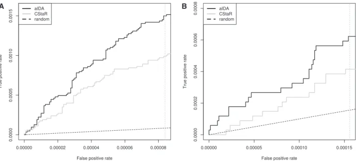
We ran aIDA and CStaR with the same 100 subsamples of the 63 observational samples. Lists of predicted causal effects were gen-erated and filtered for gene pairsðX!Y), whereXis among the 234 genes, for which deletion strain data was available. The inter-ventional data from deletion strains were used to classify these pre-dictions into true and false positive prepre-dictions.Figure 7A shows ROC curves up to 100 false positives for CStaR and aIDA, respect-ively. Again, aIDA outperforms CStaR.

4.3.2 Application to data fromLenstraet al. (2011)

Next, we used a biological dataset fromLenstraet al.(2011). This data has not been used previously for causal discoveries.Lenstra

et al.(2011)analyzed mutants of chromatin machinery components to examine the interactions between chromatin and gene expression inS.cerevisiae.Following preprocessing, the data consisted of 138 interventional single-gene deletion profiles and 67 observational wild type samples (for details on data preprocessing see Supplementary Materials Section 3.3).Figure 7B shows that also on this dataset, causal discovery is possible. As can be seen from this Figure, aIDA again performs better in comparison to CStaR.

5 Discussion

We presented aIDA, a method to estimate causal effects from obser-vational data in situations where we have many variables but only few observations, a common situation in biology due to costs of the experiments and availability of biomaterial. aIDA does not require any knowledge about the causal network underlying the data. It uses IDA in a subsampling approach (Maathuiset al., 2009) to ac-count for small sample sizes. While IDA and CStaR take the Fig. 5.Comparison of the partial area under the ROC curve up to 100 false

positives for 10 simulated datasets with 100 nodes, andn¼50 andn¼1000 samples. Black bars show values for aIDA, gray bars show values for CStaR. The error bars indicate standard errors across the 10 datasets

Fig. 6.Comparison of the partial area under the ROC curve up to 100 false positives for the 5 simulated datasets with 1000 nodes,n¼50 samples, a

¼0:5 and a dense and a sparse underlying true graph, respectively. Black bars show values for aIDA, gray bars show values for CStaR. The error bars indicate standard errors across the 5 datasets

(7)

minimum absolute value of causal effects fromKsubsampling runs (Maathuiset al., 2009,2010;Stekhovenet al., 2012), aIDA uses the whole multisets of causal effects. The estimate for the true causal ef-fect is the mode of the density calculated over all estimated sets of causal effects acrossKsubsampling runs.

IDA and all its extensions require among other assumptions that the multivariate Gaussian distribution is faithful to the DAG (Kalisch and Bu¨hlmann, 2007), i.e. statistical conditional indepen-dencies can be inferred from the underlying DAG. Faithfulness in general is not testable (Zhang and Spirtes, 2008) and, of course, there is no evolutionary selection pressure that makes biological networks faithful. An additional limitation of all existing approaches for causal discovery is that feedback mechanisms not be captured by a DAG. Therefore, IDA, CStaR and aIDA can-not replace wet lab experiments, but are a good starting point for experimental design.

We show that aIDA outperforms CStaR on both simulated and real datasets with respect to the partial area under the receiver oper-ating characteristics (ROC) curve up to 100 false positives. Besides yielding improved estimates of the top candidates for intervention experiments, the results on simulated data suggest that aIDA per-forms better than existing algorithms on small sample sizes. In sum-mary aIDA improves the estimation of causal effects from observational data. These findings suggest aIDA as a useful tool for experimental design of functional studies.

Acknowledgement

We thank Peter Oefner and Maurits Evers for valuable discussions.

Funding

This work was funded by the Bavarian Research Network for Molecular Biosystems (BioSysNet) and by the e:bio initiative of the German Federal Ministry of Education and Research (BMBF), grant number 0316166G.

Conflict of Interest: none declared.

References

Balaji,S.et al. (2006) Comprehensive analysis of combinatorial regulation using the transcriptional regulatory network of yeast.J. Mol. Biol.,360, 213–227.

Baudin,A.et al. (1993) A simple and efficient method for direct gene deletion inSaccharomyces cerevisiae.Nucleic Acids Res.,21, 3329–3330. Chickering,D. (1996) Learning Bayesian networks is NP-complete. In:

Fisher,D. and Lenz,H.-J. (eds.)Learning from Data: Artificial Intelligence and Statistics V. Springer, New York.

Chickering,D.M. (2002) Learning equivalence classes of Bayesian network structures.J. Mach. Learn. Res.,2, 445–498.

Colombo,D. and Maathuis,M.H. (2012) A modification of the pc algorithm yielding order-independent skeletons.CoRR,abs/1211.3295.

Dash,D. and Druzdzel,M.J. (1999) A hybrid anytime algorithm for the con-struction of causal models from sparse data. In: Laskey,K.B. and Prade,H. (eds.)UAI. Morgan Kaufmann, Publishers, San Francisco, CA, USA, pp. 142–149.

Fire,A.et al. (1998) Potent and specific genetic interference by double-stranded RNA inCaenorhabditis elegans.Nature,391, 806–811.

Goldszmidt,M. and Pearl,J. (1992) Rank-based systems: a simple ap-proach to belief revision, belief update, and reasoning about evidence and actions. In: Nebel,B. et al (eds.) Proceedings of the Third International Conference on Principles of Knowledge Representation and Reasoning, pp. 661–672.

Hughes,T.R.et al. (2000) Functional discovery via a compendium of expres-sion profiles.Cell,102, 109–126.

Huynh-Thu,V.A.et al. (2010) Inferring regulatory networks from expression data using tree-based methods.PLoS ONE,5, e12776þ.

Kalisch,M. and Bu¨hlmann,P. (2007) Estimating high-dimensional directed acyclic graphs with the pc-algorithm. J. Mach. Learn. Res.,8, 613–636.

Kalisch,M.et al. (2012) Causal inference using graphical models with the R package pcalg.J. Stat. Softw.,47, 1.

Larson,M.H.et al. (2013) CRISPR interference (CRISPRi) for sequence-spe-cific control of gene expression.Nat. Protocols,8, 2180–2196.

Lenstra,T.L.et al. (2011) The specificity and topology of chromatin inter-action pathways in yeast.Mol. Cell,42, 536549.

Maathuis,M.H.et al. (2009) Estimating high-dimensional intervention effects from observational data.Ann. Stat,37, 3133–3164.

A

B

Fig. 7.ROC curves for theHugheset al.(2000)and theLenstraet al.(2011)dataset up to 100 FP usinga¼0.5. The solid black curves represent the ROC curves for aIDA, the gray curves show the ROC curves for CStaR, and the dotted black lines refer to random guessing. (A) While both methods perform better than random guessing, aIDA shows better performance up to 100 FP than CStaR for the dataset fromHugheset al.(2000). (B) aIDA improves over CStaR for the dataset from

Lenstraet al.(2011). aIDA performs better than random guessing, while CStaR at the beginning of the ranked list does not

(8)

from observational data.Nat. Methods,7, 247–248.

Madigan,D.et al. (1996) Bayesian model averaging and model selection for Markov equivalence classes of acyclic digraphs. Communications in Statistics: Theory and Methods,25, 2493–2519.

Margolin,A.A.et al. (2006) Aracne: an algorithm for the reconstruction of gene regulatory networks in a mammalian cellular context.BMC Bioinformatics, 7(Suppl 1): S7.

Meek,C. (1995) Causal inference and causal explanation with background knowledge. In: Besnard,P. and Hanks,S. (eds.)UAI, Morgan Kaufmann, Publishers, San Francisco, CA, USA, pp. 403–410.

Meinshausen,N. and Bu¨hlmann,P. (2010) Stability selection.J. R. Stat. Soc. Ser. B (Statistical Methodology),72, 417–473.

Pearl,J. (1988) Probabilistic Reasoning in Intelligent Systems. Morgan Kaufmann, Publishers, San Francisco, CA, USA.

Pearl,J. (1995) Causal diagrams for empirical research.Biometrika,82, 669.

University Press, Cambridge, UK.

Spirtes,P. et al. (2000) Causation, Prediction, and Search. MIT press, Cambridge, MA, USA, 2nd edn.

Stekhoven,D.J.et al. (2012) Causal stability ranking. Bioinformatics,28, 2819–2823.

Tian,J. and Pearl,J. (2002) A general identification condition for causal effects. In: Dechter,R. and Sutton,R.S. (eds.)AAAI/IAAI, AAAI Press/The MIT Press, Cambridge, MA, USA, pp. 567–573.

Verma,T. and Pearl,J. (1991) Equivalence and synthesis of causal models. In: Bonissone, P.P.et al. (eds.)UAI, Elsevier, Science Publishers B.V., Atlanta, GA, USA, pp. 255–270.

Wach,A. (1996) PCR-synthesis of marker cassettes with long flanking hom-ology regions for gene disruptions inS. cerevisiae. Yeast,12, 259–265. Zhang,J. and Spirtes,P. (2008) Detection of unfaithfulness and robust causal

inference.Minds Mach.,18, 239–271.

Supplementary material.