Unsupervised Discovery of El Ni ˜no
Using Causal Feature Learning on Microlevel Climate Data
Krzysztof Chalupka Computation and Neural Systems
Caltech Tobias Bischoff Environmental Science and Engineering Caltech Pietro Perona Electrical Engineering Caltech Frederick Eberhardt Humanities and Social Sciences
Caltech
Abstract
We show that the climate phenomena of El Ni˜no and La Ni˜na arise naturally as states of macro-variables when our recent causal feature learn-ing framework (Chalupka et al., 2015, 2016) is applied to micro-level measures of zonal wind (ZW) and sea surface temperatures (SST) taken over the equatorial band of the Pacific Ocean. The method identifies these unusual climate states on the basis of the relation between ZW and SST patterns without any input about past occurrences of El Ni˜no or La Ni˜na. The sim-pler alternatives of (i) clustering the SST fields while disregarding their relationship with ZW patterns, or (ii) clustering the joint ZW-SST pat-terns, do not discover El Ni˜no. We discuss the degree to which our method supports a causal interpretation and use a low-dimensional toy ex-ample to explain its success over other cluster-ing approaches. Finally, we propose a new ro-bust and scalable alternative to our original algo-rithm (Chalupka et al., 2016), which circumvents the need for high-dimensional density learning.
1
INTRODUCTION
The accurate characterization of macro-level climate phe-nomena is crucial to an understanding of climate dynam-ics, long term climate evolution and forecasting. Modern climate science models, despite their complexity, rely on an accurate and valid aggregation of micro-level measure-ments into macro-phenomena. While many aspects of the climate may indeed be subject fundamentally to chaotic dy-namics, many large scale phenomena are deemed amenable to precise modeling. The El Ni˜no–Southern Oscillation (ENSO) is arguably the most studied climate phenomenon at the inter-annual time scale, but much about its dynam-ics relating zonal winds (ZW) and sea surface temperatures (SST) remains poorly understood.
Figure 1: El Ni˜no vs. neutral conditions from Di Liberto (2014). Top: An illustration of the state of the atmosphere and surface during typical El Ni˜no conditions. Here, the colors indicate SST deviations from the neutral state with red being a positive and blue being a negative deviation. Bottom: Similar to the top panel but now showing neutral conditions of the Walker circulation (neither El Ni˜no nor La Ni˜na).
We apply our recent causal feature learning (CFL) frame-work (Chalupka et al., 2016) to learn causal macro-variables from the equatorial Pacific climate data. Our goal is threefold:
• apply CFL to real-world data, developing new practi-cal algorithms as needed,
• test whether CFL can, without supervision, learn the ground truth that El Ni˜no is an important macro-variable state in the ZW-SST system’s dynamics, • explore the theoretical and practical difference
be-tween CFL and clustering methods.
From the climate-science point of view, our research shows
Figure 2: Ni˜no 3.4 SST anomalies for the time period 1950–2005. The figure was adapted from McPhaden et al. (2006). Red shadings indicate El Ni˜no years and blue shad-ings indicate La Ni˜na years. The two dashed lines indicate the threshold for strong El Ni˜no or La Ni˜na events. that CFL can be successfully used for an unbiased auto-mated extraction of climate macro-variables, which would otherwise require tedious hand-crafting by domain experts. Moreover, the framework can directly suggest (compu-tationally) expensive climate experiments (for example, through climate simulations) that could differentiate be-tween true causes and mere correlations efficiently. Closer inspection of the output of CFL can also yield insights about new climate macro-phenomena (or important vari-ants of existing ones) that inspire new physical mod-els of the climate. Python code that reproduces our re-sults and figures is available online athttp://vision. caltech.edu/˜kchalupk/code.html.
1.1 EL NI ˜NO–SOUTHERN OSCILLATION
El Ni˜no is a weather pattern that is principally charac-terized by the state of eastern Pacific near-surface winds (ZW, zonal wind), sea surface temperature (SST) patterns, and the associated state of the atmospheric Walker circula-tion (see for example, Holton et al., 1989; Trenberth, 1997). The Walker circulation (see Fig. 1) is characterized by warm air rising over Indonesia and Papua New Guinea and cooler subsiding air over the eastern Pacific cold tongue re-gion just west of equatorial South America (Lau and Yang, 2003). Near the surface, easterly winds (winds blowing from the east) drive water from east to west resulting in oceanic upwelling near the coast of equatorial South Amer-ica (and downwelling east of Indonesia), that brings with it cold and nutrient rich waters from the deep oceans. During the ENSO warm phase, commonly referred to as El Ni˜no (because it often occurs around and after Christmas), the Walker circulation weakens, ultimately resulting in weaker upwelling in the Eastern Pacific and thus in positive SST anomalies. Fig. 1 illustrates these phenomena.
ENSO-related weather in the tropics includes droughts, flooding, and may have direct impact on fisheries through reduced nutrient upwelling (e.g., Glantz, 2001).
Atmo-spheric waves (ripples in wind, SST and rainfall pat-terns) generated by the change in circulation and SST anomalies in the tropics, make their way across the planet with dramatic impact (e.g, Ropelewski and Halpert, 1987; Changnon, 1999). Cashin et al. (2015) show that the eco-nomic impact of El Ni˜no varies across regions. Ecoeco-nomic activity may decline briefly in Australia, Chile, Indonesia, India, Japan, New Zealand, and South Africa after an El Ni˜no event. Enhanced growth may be registered in other countries, such as the United States.
The ENSO cold phase, usually referred to as La Ni˜na, is the opposing phase of El Ni˜no with enhanced upwelling and colder SSTs in the eastern Pacific. Currently, predict-ing the strength of El Ni˜no and La Ni˜na events remains a difficult challenge for climate scientists as the period may vary between 3 and 7 years (see Fig. 2); as a consequence accurate forecasts are only possible less than a year in ad-vance (e.g., Landsea and Knaff, 2000).
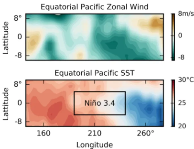
The National Oceanic and Atmospheric Administration (NOAA) defines El Ni˜no as a positive three-month run-ning mean SST anomaly of more than 0.5◦C from nor-mal (for the 1971–2000 base period) in the Ni˜no 3.4 re-gion (120◦W–170◦W, 5◦N–5◦S, see also Fig. 4). Simi-larly, La Ni˜na conditions are defined as negative anoma-lies of more than−0.5◦C. Conditions in between−0.5◦C and0.5◦C are called neutral. This is illustrated using red and blue shadings in Fig. 2. Strong El Ni˜no/La Ni˜na events are defined as SST-anomalies greater than1.5◦C. However, the definitions for El Ni˜no and La Ni˜na have evolved over time. For example, other regions than the Ni˜no 3.4 region or other averaging conventions have been used in the spec-ification of the SST anomalies.
1.2 CAUSAL FEATURES AND MACRO-VARIABLES
Climate experts view zonal winds as drivers of SST pat-terns. We take the view that if El Ni˜no and La Ni˜na are indeed genuine macro-level climate phenomena in their own right (and not just arbitrary quantities defined by con-vention) then they must consist of macro-level features of the relation between the high-dimensional micro-level ZT and SST patterns that can be detected by an unsupervised method. That is, it must be possible to identify El Ni˜no and La Ni˜na from a mass of air pressure and sea temperature readings, using a method that has no independent informa-tion about when such periods occurred.
In Chalupka et al. (2016) we developed a theoretically pre-cise account of causal relations of macro-variables that su-pervene on micro-variables, and proposed an unsupervised method for their discovery, which we called Causal Fea-ture Learning (CFL). We adopt the framework (summa-rized below) with a few interpretational adjustments for our climate setting. The method (originally inspired by
the neuroscience setting, only tested on synthetic data) was designed to establish claims such as“The presence of faces (in an image) causes specific neural processes in the brain.”, where a neural process identifies a class of spike trains across a large number of neurons recorded by elec-trodes. An ability to characterize such neural processes would provide the basis to explain, for example, what con-stitutes face recognition in the brain. There we considered as input visual stimuli (in the form of still images) and as output electrode recordings of the neural response of 1000 neurons (in the form of spike trains).
Formally, let an input (micro-)variable X take values in a high-dimensional domainX (in Chalupka et al. (2016), the pixel space of an image, in our case here ZW maps) and the output (micro-)variableY take values in the high-dimensional domain Y (the space of neural spike trains then, the SST patterns here). The basic idea underlying our set-up is that the causal macro-variable relation is de-fined in terms of the coarsest aggregation of the micro-level spaces that preserves the probabilistic relations un-der intervention (hence, causal) between the micro-level spaces. Conceptually, macro-level causal variables group together micro-level states that make no causal difference. In Chalupka et al. (2016) we started by defining a micro-level manipulation (similar to Pearl’sdo()-operator (Pearl, 2000)):
Definition 1 (Micro-level Manipulation). A micro-level manipulationis the operationman(X =x)that changes the value of the micro-variableX tox∈ X, while not (di-rectly) affecting any other variables. We writeman(x)if the manipulated variableX is clear from context.
The micro-level manipulation is then used to define what we refer to as thefundamental causal partition:
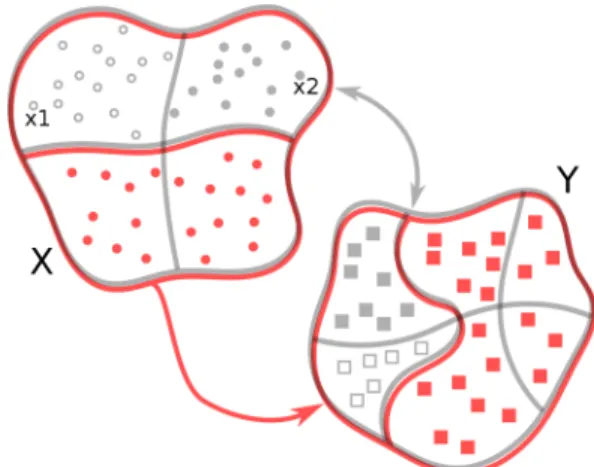
Definition 2(Fundamental Causal Partition, Causal Class).
Given the pair(X,Y), thefundamental causal partition of X, denoted byΠc(X)is the partition induced by the equiv-alence relationX∼such that
x1
X
∼x2 ⇔ ∀yP(y|man(x1)) =P(y|man(x2)).
Similarly, thefundamental causal partition ofY, denoted by
Πc(Y), is the partition induced by the equivalence relation Y
∼such that
y1
Y
∼y2 ⇔ ∀xP(y1|man(x)) =P(y2|man(x)).
A cell of a causal partition is acausal classofXorY.
The fundamental causal partitions then naturally give rise to the macro-level cause variableCand effect variable E
that stand in a bijective relation to the cells ofΠc(X)and
Πc(Y), respectively. Thus, the macro-variable causeC
ig-nores all the micro-level changes in X that do not have an effect on the probabilities over Y, and the macro-level
Figure 3: The Causal Coarsening Theorem, adapted from Chalupka et al. (2016). In this plot, theobservationalinput macro-variable (top, gray) has four states, and has a well-defined joint with the observational output macro-variable (with six states). In each case, thecausalmacro-variable states are a coarsening of the observational states. For ex-ample, the input causal macro-variable merges the two top observational states. E.g. P(Y | x1) =6 P(Y | x2), but
P(Y |man(x1)) =P(Y |man(x2)).
effectE ignores all the micro-level detail inY, which oc-cur with the same probability given a manipulation to any
X =x.
With these definitions there is no reasona priorito think that macro-variables are common phenomena. In fact quite the opposite: The conditions that the probability distri-butions over X and Y must satisfy to give rise to non-trivial macro-variablesCandEcan easily be described as a measure-zero event when taken in their strict form. Conse-quently, our view is that to the extent that macro-variables are discussed in a scientific domain, there must be a pre-supposition that such strong conditions are satisfied at least approximately.
In the present context, our climate data consisting of ZW and SST measurements (we give a detailed description of the data in Section 1.3 below) is entirely observational. That is, the data is naturally sampled fromP(SST, ZW)
and not created by a (hypothetical) experimentalist from
P(SST|man(ZW=z))for different values ofz. Never-theless, we can identify theobservationalmacro-variables that characterize the probabilistic relation between ZW and SST by replacing the probabilities in Definition 1.2 with observational probabilitiesP(y|x):
Definition 3(Fundamental Observational Partition, Obser-vational Class). Given the pair (X,Y), the fundamental observational partition ofX, denoted byΠo(X)is the par-tition induced by the equivalence relation∼Xsuch that
x1
X
∼x2 ⇔ ∀y P(y|x1) =P(y|x2).
de-Figure 4: A micro-variable climate dataset. Top: A week’s average ZW field. Bottom: A week’s average SST field over the same region. In addition, the Ni˜no 3.4 region is marked. Our dataset comprises 36 years’ worth of overlap-ping weekly averages over the presented region.
noted byΠo(Y), is the partition induced by the equivalence relation∼Y such that
y1
Y
∼y2 ⇔ ∀xP(y1|x) =P(y2|x).
A cell of an observational partition is an observational classofXorY.
In Chalupka et al. (2016) we showed that the fundamen-tal causal partition is almost always a coarsening of the corresponding fundamental observational partition, as il-lustrated in Fig. 3. We thus have some reason to expect that any macro-variables we do identify from our observational climate data will capture all the distinctions that are causal, but may in addition make some distinctions that do not sup-port a causal inference. We return to this point in Section 6, where we discuss in more detail what causal insights can be drawn from this work. Our results should be seen as a step towards a characterization of macro-level causal vari-ables for climate science, but we fully acknowledge that a complete causal characterization of the equatorial Pacific climate dynamics is beyond the scope of this paper.
1.3 DATASET
The data used for this study is based on the daily-averaged version of the NCEP-DOE Reanalysis 2 prod-uct for the time period 1979–2014 inclusive (Kanamitsu et al., 2002), a data product provided by the US National Centers for Environmental Protection (NCEP) and the De-partment of Energy (DOE). Reanalysis data sets are gen-erated by fitting a complex climate model to all avail-able data for a given period of time, thus generating es-timates for times and locations that were not originally observed. In addition, we used the Geophysical
Obser-vational Analysis Tool (http://www.goat-geo.org) to inter-polate the SST and zonal wind fields onto a 2.5◦×2.5◦
spatial grid for easier analysis. We chose to focus on the (140◦, 280◦)E×(-10◦, +10◦)N equatorial band of the Pa-cific Ocean. From the raw dataset, we extracted the zonal (west-to-east) wind component and SST data in this region (specifically, we extracted the fields at the1000hPa level near the surface). Finally, we smoothed the data by com-puting a running weekly average in each domain. The re-sulting dataset contains 13140 zonal wind and 13140 cor-responding SST maps, each a 9×55 matrix. Fig. 4 shows sample data points.
2
PACIFIC MACRO-VARIABLES
To apply CFL in practice, we adapted our unsupervised causal feature learning algorithm (Chalupka et al., 2016) to more realistic scenarios. The new solution (Sec. 3) is more robust and applicable to high-dimensional real-world data. We start with a description of the results.
Throughout the article, we will refer to zonal wind macro-variables as W, and to temperature macro-variables as T. We first chose to search for four-state macro-variables (though we experiment with varying this number in Sec. 4.1) and considered a zero-time delay1 between W
and T. In the CFL framework, each macro-variable state corresponds to a cell of a partition of the respective micro-variable input space. Fig. 5 visualizes the W and T we learned by plotting the difference between each macro-variable cell’s mean and the ZW (SST) mean across the whole dataset. The visualized states are easy to describe: For example, when W=WEqt there is a larger-than-average westerly wind component in the west-equatorial region, a feature often associated with the causes of El Ni˜no (see Fig. 1). Indeed, Table 1 shows that the El Ni˜no cell of T only arises in connection with W=WEqt. In addition, WEqt is often positively correlated with the T=Warm. Through-out the rest of the article, we will mostly focus on the T macro-variable. Our first goal is to quantitatively justify calling T=1 “El Ni˜no” and calling T=2 “La Ni˜na”. Quali-tatively, the warm and cold water tongues that reach west-ward across the Pacific and that are often used to describe the two phenomena, are evident in the image.
Following the standard definition of El Ni˜no (see Sec-tion 1.1), we use the SST anomaly in the Ni˜no 3.4 region to detect its presence (Trenberth, 1997). The anomaly is com-puted with respect to the climatological mean, that is the 1A zero time delay implies that CFL will attempt to relate the
weekly moving ZW average to the weekly moving SST average. The question of different time delays turns out to be a very subtle issue in the study of El Ni˜no as El Ni˜no is not a periodic event, nor does it have a fixed duration (see Fig. 2). A careful discussion of other delays is not feasible in a short article and the zero-time delay was deemed a reasonable starting point by domain experts we consulted.
Figure 5: Macro-variables discovered by Alg. 1. For each state, the average difference from the dataset mean is shown. Left: Four states of W, the zonal wind macro-variable. We named the states “Easterly Equatorial” (EEqt),“Westerly Equatorial” (WEqt), “Easterly North of Equator” (EN) and “Easterly South of Equator” (ES). Right: Four states of T, the SST macro-variable. We named the states “Cold [American Coastal Waters]”, “El Ni˜no”, “La Ni˜na” and “Warm [American Coastal Waters]”. The main text provides additional justification for calling T=1 and T=2 “El Ni˜no” and ”La Ni˜na”, respectively.
mean temperatureduring the same week of the yearover all the weeks in our dataset. We will call a weekly average anomaly exceeding +.5◦C a mild episode, and an anomaly exceeding +1.5◦C a strong episode. The definition of La Ni˜na is analogous, with negative thresholds. Fig. 6 shows that in the T=1 and T=2 cells, over 75% of all the points exceed the threshold for a mild (positive and negative, re-spectively) anomaly, and over50%of the points exceed the strong threshold. The situation is different in the Warm and Cold cells, where almost no points exceed the strong threshold while the number of points falling in these non-anomalous cells is about 30% of the total. Since this macro-variable contains a state capturing a high proportion of El Ni˜no-like patterns, we will say that this state has a “high precision” of detecting El Ni˜no, while similarly, state T=2 has a high La Ni˜na precision. Formally, we define the pre-cision of a macro-variable state as follows:
Definition 4(precision). LetT ={T1,· · ·, TK}be a par-tition of the set of all the SST maps used in our experiments. Let n34 : SST → Rbe the function that computes the
Ni˜no 3.4 anomaly for a given map. Then, let
cθ(Tk) = 1 |Tk||{t∈Tk s.t. n34(t)> θ}| ifθ >0 1 |Tk||{t∈Tk s.t. n34(t)< θ}| ifθ <0 be the function that computes for, a given cell Tk of the partition, the fraction of its members whose anomaly is greater than (if θ > 0) or lesser than (ifθ < 0) a given thresholdθ. Finally, call the four numbers maxkc.5(Tk),
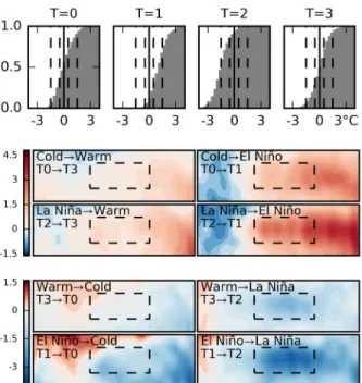
Figure 6: T=1 and T=2 are El Ni˜no and La Ni˜na. Top: Each plot shows the cumulative histogram of the Ni˜no 3.4 anomalies, computed over all the weekly SST averages that belong to the given state of T. The dashed lines show the +/-0.5 and +/-1.5 “mild” and “strong” anomaly thresholds. Bottom: The minimal manipulations needed to transition from a given T-state into another (the exact procedure to obtain the plots is described in the text).
maxkc1.5(Tk), maxkc(−.5)(Tk), maxkc(−1.5)(Tk) the mild/strong-El Ni˜no and mild/strong-La Ni˜na precision of the macro-variableT.
Together, the precisions indicate how well the partition T separates the mild and strong El Ni˜no and La Ni˜na anoma-lies from other structures in the data. In Fig. 6, for ex-ample, c.5(T) ≈.75andc1.5(T)≈ .25(both because of
T=1),c(−.5)(T)≈.85andc(−1.5)(T)≈.5(both because
of T=2). Thus, T has high mild-El Ni˜no precision, and high mild-La Ni˜na precision.
As further evidence that Alg. 1 recovered El Ni˜no and La Ni˜na, we show minimal state-to-state manipulations in Fig. 6. Take the La Ni˜na→El Ni˜no plot as an example. To compute it, we took all the SST maps for which T=La Ni˜na, and for each foundthe closest(in the Euclidean space) map for which T=El Ni˜no. We then averaged these differences. One of the insights the figure offers is that low SSTs in the Ni˜no 3.4 region really are the distinguishing feature of T=La Ni˜na. Similarly, an important difference between the T=Warm and T=El Ni˜no is the characteristic tongue of warm water extending into the Ni˜no 3.4 region. Adding this tongue is necessary to switch from T=Cold to T=El Ni˜no, but not to switch from T=Cold or T=La Ni˜na to T=Warm. The CFL framework allows us to interpret W and T as
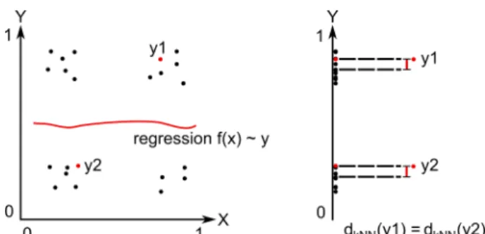
stan-Figure 7: Alg. 1 vs. clustering. In this toy example, the data is sampled from the distributionP(X) =U({1/5; 2/5)} ∪ {3/5; 4/5}), P(Y | X) = P(Y) = U({1/5; 2/5)} ∪ {3/5; 4/5}). The clusters in the X, Y, and joint X,Y space are evident. However, since X and Y are inde-pendent, we expect Alg. 1 to find only one macrolevel class ofX. Indeed, (properly regularized) regression gives
f(x) =const∀x, soW(x) = 0∀x. Incidentally, since the
density ofY is similar in the neighborhood of each sample
y(see data Y-projection on the right),T(y) = 0∀y.
dard probabilistic random variables with distribution we can estimate. Table 1 offers a probabilistic description of the system we learned. “When the equatorial zonal wind is unusually westerly, there is a 75% chance that the eastern Pacific is warm, and a 25% chance that El Ni˜no arises.” and “When the North-equatorial zonal wind is predominantly westerly, but the South-equatorial easterly, then the East-ern Pacific is most likely to be cold.”—are example insights about the equatorial Pacific wind-SST system offered by CFL. We emphasize that both the macro-variables and the probabilities are learned from the data in an entirely un-supervised manner, without any a priori input about what constitutes ENSO events (except the fact that we restrict the SST and ZW fields to the equatorial Pacific region).
3
CFL: A ROBUST ALGORITHM
The practical bottleneck of the original CFL algo-rithm (Chalupka et al., 2016) is the need for joint den-sity estimation of p(X, Y). Density estimation is noto-riously hard, especially in high dimensions. We modified the original algorithm to avoid explicit density estimation. An additional advantage of our approach (Alg. 1) is that it is very robust with respect to input space dimensional-ity: Input data is only used explicitly in regression, which can be implemented using any algorithm that easily handles high-dimensional inputs (we used neural nets).
LetX,Ydenote the micro-variable input and output space, respectively. Our algorithm is based on the insight that CFL only needs to detect the two equivalences
p(Y |x1) =p(Y |x2)for anyx1, x2∈ X and (1)
p(y1|x) =p(y2|x)for anyy1, y2∈ Y, x∈ X, (2)
instead of actually computing the conditionalsp(Y |X).
Algorithm 1:Unsupervised Causal Feature Learning input :D={(x1, y1),· · ·,(xN, yN)}
Cluster– a clustering algorithm
output:W(x), T(y)– the causal class of eachx, y.
1 Regressf ←argminfΣi(f(xi)−yi)2; 2 LetW(xi)←Cluster(f(x1),· · ·, f(xN))[xi]; 3 LetRange(W) ={0,· · ·, N}; 4 LetYw← {y|W(x) =wand(x, y)∈ D}; 5 Letg(y)←[kNN(y,Y0),· · · ,kNN(y,YN)]; 6 LetT(yi)←Cluster(g(y1),· · ·, g(yN))[yi];
If Eq. (1) holds, we also have E[Y | x1] = E[Y | x2].
Computing conditional expectations is much easier than learning the full conditional:f(X) =E[Y |X]minimizes E[(Y −f(X))2], so learning the conditional expectation amounts to regressingY onXunder the mean-squared er-ror measure. Unfortunately, equal conditional expectations do not imply equal conditional distributions. However, ar-guably the practical risk of encountering differing condi-tionals with identical means is lower than the risk of failing at high-dimensional density learning. For this reason, we useE[Y |x1] = E[Y |x2]as a heuristic indicator of the
equivalence of the conditionals in Eq. (1) (see Line 2 in Alg. 1). For a more robust heuristic one could use more than just equal expectations to decide distribution equality. A promising direction would be to use a Mixture Density Network (Bishop, 1994) to approximate P(Y | x)with a mixture of Gaussians for eachx, and then cluster the mix-tures.
Clustering the conditional expectations gives us the macro-variable class W(x) of each input x. By construc-tion (Chalupka et al., 2015), we havep(Y | x) = P(Y |
W(x))and by assumption the range ofWis small. Instead of checking whether Eq. (2) holds for a given pair y1, y2
over all the x ∈ X, it is thus enough to check whether
p(y1 | W = w) = p(y2 | W = w) for each value
w ∈ Range(W). For each givenw we have a subset Yw⊂ Ywhich consists of all they’s whose corresponding
x’s have causal classw. Consequently, Eq. (2) does not de-pend on the exact densities conditional on the micro-state, but only the densities conditional on the macro-level state. Thus, instead of trying to evaluate any given p(y | w), Line 5 computesthe distance ofyto the k-th nearest neigh-bor in Yw. This idea is based on a principle that
under-Cold El Ni˜no La Ni˜na Warm
EEqt 2/3 0 1/3 0
WEqt 0 1/4 0 3/4
EN ∼1/10 0 1/4 ∼2/3
ES 3/4 0 0 1/4
Figure 8: Changes in macro-variable precision as we vary the number of states in CFL, clustering, and CFL on reshuf-fled data (“Rand CFL”). With two states, it is impossible to differentiate El Ni˜no and La Ni˜na from other weather fea-tures, be it dynamic (CFL) or spatio-structural (clustering). Increasing the number of states reveals differences between the algorithms.
lies a whole class of nonparametric density estimation al-gorithms (Fukunaga and Hostetler, 1973; Mack and Rosen-blatt, 1979): Where the density is high, samples from the distribution are closer to each other than where the den-sity is low. This is illustrated in Fig 7. On the right, we plotted the projection of the data onto the y-space. In this projection, the distance ofy1 to its third-nearest neighbor
is roughly the same as the distance ofy2to its third-nearest
neighbor. Indeed, this is the case for all they’s, because they are generated from a distribution that assigns equal density to all of them.
In Chalupka et al. (2016) we represented eachyby an esti-mate of[p(y|x1),· · · , p(y|xN)], whereNis the number
of datapoints. The new approach represents eachy sam-ple by its ’k-nn representation’, one scalar value for each
w∈Range(W)(Line 5). Clustering these representations gives us the causal stateT(y)for eachy.
Algorithm 1 relies on a successful regressionf that mini-mizes the mean squared error E[(f(x)−y)2]. In our
ex-periments, we used the Theano (Bastien et al., 2012) and Lasagne packages to implement and train a three-hidden-layers, fully-connected neural network (Bishop, 1995) in Python. The data was sufficiently simple (compared to e.g. image datasets used to evaluate state-of-the-art neural nets in vision) that no regularization technique beyond simple weight decay and early stopping was necessary to minimize the validation error.
Figure 9: t-SNE (Van der Maaten and Hinton, 2008) em-bedding of the k-nn representation of SST data. The blue dots show, for varying K, the state of T with largestc(−.5)
precision (see Def. 4). The red dots show the state with largestc.5. Thus, the blue dots are “the” La Ni˜na cluster
for each K, and the red dots “the” El Ni˜no cluster.
4
ROBUSTNESS OF THE RESULTS
In this section, we describe two additional studies we per-formed to ensure our algorithm behaves as expected, and that the results are robust with respect to changing the ex-perimental parameters.
4.1 VARYING THE NUMBER OF STATES
Our choice of discovering four-state macro-variables was rather arbitrary. To check how varying the number of states changes the macro-variable precision (Def. 4), we repeated our experimental procedure, varying the number of states K from 2 to 16 (both in the ZW and SST space). Fig. 8 shows the precisions for each case. As expected, a low number of states (K=2, 3) doesn’t allow the algorithm to precisely detect El Ni˜no and La Ni˜na. With K>4 however, a slowly growing trend persists at high precision values. El Ni˜no and La Ni˜na remain important features as K changes. There are several possible behaviors of the algorithm given the slowly growing precision of the macro-variables with growing K: (1) The El Ni˜no and La Ni˜na states remain roughly constant, (2) CFL sub-divides the El Ni˜no and La Ni˜na states, (3) CFL finds better El Ni˜no and La Ni˜na re-gions, (3) A mix of the above. Fig. 9 suggests that (2) is true. As K grows, the clusters that most precisely detect the mild El Ni˜no and mild La Ni˜na phenomena form a chain of strict subsets.
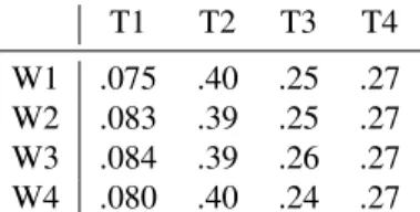
T1 T2 T3 T4 W1 .075 .40 .25 .27 W2 .083 .39 .25 .27 W3 .084 .39 .26 .27 W4 .080 .40 .24 .27
Table 2: Conditional probabilitiesP(T |W)when Alg. 1 is applied to randomly (in time) reshuffled ZW and SST data.
4.2 RESHUFFLED DATA
As a sanity check, we ran Alg. 1 on randomly reshuf-fled (across the time dimension) ZW and SST data. We asked the algorithm to find K=4, . . . , 16-state ZW and SST macro-variables. Table 2 shows P(T | W), where
W andT are the input and output macro-variables discov-ered in the randomized dataset with K = 4. Note that
P(T | W =W1),P(T |W =W2),P(T |W =W3)
andP(T | W =W4)are all equal. This is exactly as ex-pected, since by reshuffling the data we removed any prob-abilistic dependence between the inputs and the outputs. Applying Definition 2 to this data indicates that the al-gorithm implicitly only discovered one true input state, even though we explicitly asked it to look for a four-state variable. The cardinality of the output macro-variable is three or four states, depending on whether.25
is close enough to .27 to apply Def. 2 to merge the last two columns. We performed the same reshuffled analysis for each K and computed as before the precision for the weak and strong El Ni˜no and the weak and strong La Ni˜na. Fig. 8, large dotted lines, shows that in each case none of the clusters contains a significant proportion of either El Ni˜no or La Ni˜na patterns. This experiment offers two in-sights:
• Alg. 1 passes the sanity check. When the inputs and outputs are independent, the input macro-variable is trivial, it has a single state.
• When SST patterns are clustered according to their probability of occurrence (e.g. as theW variable does in Table 2), El Ni˜no and La Ni˜na are not identified as macro-level climate states. We will return to this point in the Discussion.
5
WHY NOT NAIVE CLUSTERING?
It is instructive to compare our results with unsupervised clustering. Fig. 8 shows the precision coefficients for k-means clustering with k=4, . . . , 16 (small dotted line), alongside our CFL results. Whereas CFL detects both El Ni˜no and La Ni˜na with high precision using only four states, k-means struggles to achieve a similar result even for larger K.
Barring particularities of the data (which we consider in the Discussion), there is in general no reason for CFL to
give the same results as clustering. Consider the example in Fig. 7. Arguably, a reasonable clustering algorithm should find four linearly separable clusters in the jointX,Yspace, and two clusters in the X and Y space each. However, the variables are probabilistically independent. In contrast, CFL would only find a one-state input variable, since all values ofXimply the same distribution overY. Addition-ally, sinceP(Y | X) = P(Y)is constant across all the samples, CFL would also only find a one-state output vari-able. The figure illustrates that Alg. 1 does precisely that (as should the original algorithm in Chalupka et al. (2016)).
6
DISCUSSION
The CFL framework we developed in Chalupka et al. (2015, 2016) aspires to solve an important problem in causal reasoning: how to automatically form macro-level variables from micro-level observations. In this work we have shown, for the first time, that these algorithms can be successfully applied to real-life data. We have recov-ered well-known, complex climate phenomena (El Ni˜no, La Ni˜na) as macro-variable states directly from climate data, in an entirely unsupervised manner. In order to do so, we developed a new, practical version of the original CFL algorithm.
We emphasize that our experiments useobservational cli-mate data, and we have to be cautious about causal conclu-sions. It is not even cleara prioriwhether theZW →SST
causal direction is a reasonable choice: it is known that wind patterns cause changes in SST and it in turn affects the wind by changing the atmospheric pressure. Feedback loops are commonplace in climate dynamics.
The Causal Coarsening Theorems in Chalupka et al. (2015, 2016) provide the basis for an efficient learning of causal relationships based on observational macro-variables – but some experiments are required. In addition, the theorems were only shown to hold for variables that are not subject to feedback. However, we are hopeful that an extension accounting for feedback can be proven. While real cli-mate experiments are generally not feasible, such a theo-rem would provide the basis to perform large-scale climate experiments with detailed climate models, for example, to check whether interventionallyshifting from theW = 0
zonal wind state toW = 1in the climate model increases the likelihood of El Ni˜no (i.e. of SST ending up in state T=1). Connecting the CFL framework with such experi-ments is an exciting future direction as it would also enable the possibility of using the macro-variables we have found to inform policy that aims to influence climate phenomena. Our experiments that compare CFL with clustering showed that, as the number of clusters grows, k-means approaches never exceed CFL’s precision in detecting El Ni˜no and La Ni˜na. One explanation for this finding is that while clus-tering looks for spatial features in the data, CFL looks
for relational probabilistic features. Fig. 8 suggests that when the number of clusters is small there are strong spa-tial features in the data that supersede El Ni˜no and La Ni˜na in their distinctiveness. In contrast, CFL already de-tects El Ni˜no with high precision with only four clusters. This indicates that either (1) There is something unique aboutP(El Ni˜no| W)andP(La Ni˜na|W), or (2) There is something unique about P(El Ni˜no) and P(La Ni˜na). Since we disproved the second hypothesis in Sec. 4.2, our results overall indicate that the El Ni˜no and La Ni˜na phe-nomena do not only constitute interesting spatial features of the SST map, but are also crucially characterized by the dynamic aspect of the interplay between zonal winds and sea surface temperatures.
Even when working with purely observational data, CFL offers an important causal insight not revealed by cluster-ing methods. It guards against learncluster-ing variables with am-biguous manipulation effects (Spirtes and Scheines, 2004). An illustrative example of an ambiguous macro-variable is total cholesterol. Low density lipids (LDL, commonly called “bad cholesterol”) and high density lipids (HDL, “good cholesterol”) can be aggregated together to count to-tal cholesterol (TC), but TC has an ambiguous effect on heart disease because effects of LDL and HDL differ. The Causal Coarsening Theorem guarantees that each state of the observational macro-variable is causally unambiguous: no mixing of HDL and LDL can occur. In case of our El Ni˜no setup, this means that two ZW states within the same cell are guaranteed to have the same effect on the SST macro-variable.
Finally, we note that there still is significant debate among climate scientists about what exactly constitutes El Ni˜no and what its causes are. For example, recent research has shown that there may be multiple different types of El Ni˜no states (Kao and Yu, 2009; Johnson, 2013) that all fall under NOAA’s definition. Our results suggest that the current def-inition described in Section 1.1 coincides well with states of the probabilistic macro-variable discovered by CFL. In addition, Sec. 4.1 indicates that finer-grained structure does exist within the El Ni˜no and La Ni˜na clusters when they are analyzed from the relational-probabilistic standpoint. We leave this line of research as an important future direction.
Acknowledgements
KC’s and PP’s work was supported by the ONR MURI grant N00014-10-1-0933 and Gordon and Betty Moore Foundation.
References
F. Bastien, P. Lamblin, R. Pascanu, J. Bergstra, I. J. Goodfellow, A. Bergeron, N. Bouchard, and Y. Bengio. Theano: new features and speed improvements. Deep
Learning and Unsupervised Feature Learning NIPS 2012 Workshop, 2012.
C. M. Bishop. Neural networks for pattern recognition. Oxford university press, 1995.
Christopher M Bishop. Mixture density networks. 1994. P. A. Cashin, K. Mohaddes, and M. Raissi. Fair weather or
foul? The macroeconomic effects of El Ni˜no. 2015. K. Chalupka, P. Perona, and F. Eberhardt. Visual Causal
Feature Learning. InThirty-First Conference on Uncer-tainty in Artificial Intelligence, pages 181–190. AUAI Press, 2015.
K. Chalupka, P. Perona, and F. Eberhardt. Multi-Level Cause-Effect Systems. In The 19th International Con-ference on Artificial Intelligence and Statistics, 2016. S. A. Changnon. Impacts of 1997-98 El Ni˜no-generated
weather in the United States. Bulletin of the American Meteorological Society, 80(9):1819, 1999.
T. Di Liberto. The Walker Circulation: ENSO’s atmo-spheric buddy, 2014.
K. Fukunaga and L. D. Hostetler. Optimization of k nearest neighbor density estimates. Information Theory, IEEE Transactions on, 19(3):320–326, 1973.
M. H. Glantz. Currents of change: impacts of El Ni˜no and La Ni˜na on climate and society. Cambridge University Press, 2001.
J. R. Holton, R. Dmowska, and S. G. Philander. El Ni˜no, La Ni˜na, and the southern oscillation, volume 46. Aca-demic press, 1989.
N. C. Johnson. How many ENSO flavors can we distin-guish? Journal of Climate, 26(13):4816–4827, 2013. M. Kanamitsu, W. Ebisuzaki, J. Woollen, S.-K. Yang, J. J.
Hnilo, M. Fiorino, and G. L. Potter. NCEP-DOE AMIP-II reanalysis (r-2).Bulletin of the American Meteorolog-ical Society, 83(11):1631–1643, 2002.
H.-Y. Kao and J.-Y. Yu. Contrasting eastern-Pacific and central-Pacific types of ENSO. Journal of Climate, 22 (3):615–632, 2009.
C. W. Landsea and J. A. Knaff. How much skill was there in forecasting the very strong 1997-98 El Ni˜no? Bulletin of the American Meteorological Society, 81(9):2107–2119, 2000.
K. M. Lau and S. Yang. Walker circulation. Encyclopedia of atmospheric sciences, pages 2505–2510, 2003. Y. P. Mack and M. Rosenblatt. Multivariate k-nearest
neighbor density estimates. Journal of Multivariate Analysis, 9(1):1–15, 1979.
M. J. McPhaden, S. E. Zebiak, and M. H. Glantz. Enso as an integrating concept in earth science. Science, 314 (5806):1740–1745, 2006.
J. Pearl. Causality: Models, Reasoning and Inference. Cambridge university press, 2000.
C. F. Ropelewski and M. S. Halpert. Global and re-gional scale precipitation patterns associated with the El Ni˜no/Southern Oscillation. Monthly Weather Review, 115(8):1606–1626, 1987.
Peter Spirtes and Richard Scheines. Causal inference of ambiguous manipulations.Philosophy of Science, 71(5): 833–845, 2004.
K. E. Trenberth. The definition of El Ni˜no. Bulletin of the American Meteorological Society, 78(12):2771– 2777, 1997.
L. Van der Maaten and G. Hinton. Visualizing data using t-sne. Journal of Machine Learning Research, 9(2579-2605):85, 2008.