On Equivalence Between Network Topologies

On Equivalence Between Network Topologies

Tracey Ho

Department of Electrical Engineering California Institute of Technology

[email protected];

Michelle Effros

Departments of Electrical Engineering California Institute of Technology

[email protected];

Shirin Jalali

Center for Mathematics of Information California Institute of Technology

[email protected];

Abstract—One major open problem in network coding is to characterize the capacity region of a general multi-source multi-demand network. There are some existing computational tools for bounding the capacity of general networks, but their computational complexity grows very quickly with the size of the network. This motivates us to propose a new hierarchical approach which finds upper and lower bounding networks of smaller size for a given network. This approach sequentially replaces components of the network with simpler structures, i.e., with fewer links or nodes, so that the resulting network is more amenable to computational analysis and its capacity provides an upper or lower bound on the capacity of the original network. The accuracy of the resulting bounds can be bounded as a function of the link capacities. Surprisingly, we are able to simplify some families of network structures without any loss in accuracy.

I. INTRODUCTION

Finding the network coding capacity of networks with gen-eral topologies and communication demands is a challenging open problem, even for networks consisting of noiseless point-to-point links. Information theoretic inequalities can be used to bound network capacities, but it is in general a complex task to find the best combination of inequalities to apply. While various bounds (e.g. [1], [2], [2], [3]) can be obtained by clever choices of inequalities, we would like to have systematic general techniques for bounding the capacity in arbitrary network problems. We hope to derive these bounds in a way that allows us to bound the accuracy of the obtained bounds and to trade off tightness and computation. The LP outer bound [4], which gives the tightest outer bound implied by Shannon-type inequalities and has been implemented as the software programs Information Theoretic Inequalities Prover (ITIP) [5] and XITIP [6], has complexity exponential in the number of links in the network and can thus only be used to compute capacity bounds for relatively small problem instances. Inner bounds can be obtained by restricting attention to scalar linear, vector linear or abelian codes e.g. [7], [8], but the complexity of such approaches also grows quickly in the network size. This motivates us to seek systematic tools for bounding the capacity of a network by the capacity of another network with fewer links and characterizing the difference in capacity.

In this paper we introduce a novel approach for analyzing capacity regions of acyclic networks consisting of capacitated noiseless links with general demands. Inspired by [9], we employ a hierarchical network analysis that replaces pieces

of the network by equivalent or bounding models with fewer links. At each step of the process, one component of the network is replaced by a simpler structure with the same inputs and outputs. The model is an upper bounding model if all functions that can be implemented across the original network can also be implemented across the model. The model is a lower bounding model if all functions that can be implemented across that model can also be implemented across the given component. If the same model is both an upper bounding model and a lower bounding model for a given component, then the component and its model are equivalent. Where possible, we try to find upper and lower bounds that have identical structures, since bounding the accuracy of the resulting capacity bounds is easier when the topologies of the upper and lower bounding networks match.

The organization of this paper is as follows. Section II describes the system model. The problem of finding equivalent or bounding networks of smaller size and the properties of such networks is discussed in Section III. Sections IV and V describe a variety of operations for finding such networks. Section VI treats accuracy bounds. The networks considered in this paper are assumed to be acyclic. The effect of cycles and delay is discussed in Section VII. Finally, Section VIII concludes the paper.

II. SYSTEM MODEL

We mainly use the model and notation introduced in [10]. The network is modeled by an acyclic directed graph

N

= (

V

,

E

), where

V

and

E

⊆

V

×

V

denote the set of nodes and links, respectively. Each directed link e= (v1,v2)∈

E

represents a noiseless link of capacity Ce between the nodes

v1and v2in

N

. For each node v, let In(v)and Out(v)denote the set of incoming and outgoing links of node v respectively. We assume that the source nodes (S) and sink nodes (T) are distinct, i.e.,

S

T

T

= /0, and each source (sink) node has only outgoing (incoming) links. There is no loss of generality in this assumption since any network that violates these conditions can be modified to form a network that satisfies these conditions and has the same capacity. After these modifications, each node v∈

V

falls into one of the following categories: i) source nodes (S), ii) sink nodes (T) and iii) relay nodes (I). Relay nodes have both incoming and outgoing links, and they do not observe any external information. Their role is to facilitate data transfer from the source nodes to the sink nodes.

A subnetwork

N

_s = (

V

s,

E

_s) of network

N

= (

V

,

E

) is constructed based on a subset of relay nodes

I

_s⊂

I

as follows. The set of sources and sinks of the subnetwork

N

sare defined as

S

s={v∈

V

: v∈/

I

s,∃v′∈

I

s,(v,v′)∈

E

}, and

T

s={v∈

V

: v∈/

I

s,∃v′∈

I

s,(v′,v)∈

E

}. Then,

V

S=

S

sS

I

sS

T

s, and

E

s={e∈

E

: e= (v,v′),v,v′∈

V

s}.

A coding scheme of block length n for this network is described as follows. Each source node s∈

S

observes some message Ms ∈

X

s ={1,2, . . . ,2nRs}. Each sink node t ∈

T

is interested in recovering some of the messages that are observed by source nodes. Let β(t)⊆

S

denote the set of source nodes that the node t is interested in recovering. The coding operations performed by each node can be categorized as follows

1) Encoding functions performed by the source nodes: For each s∈

S, and e

∈Out(s), the encoding function corresponding to link e is described as

ge:

X

s→ {1,2, . . . ,2nCe}. (1) 2) Relay functions performed at realy nodes: If v∈/

S

S

T

, then for each e∈Out(v), the relay function correspond-ing to the link e is described as

ge:

∏

e′_∈In(v)

{1,2, . . . ,2nCe′} → {1,2, . . . ,₂nCe_{}. (2)}

3) Finally, for each t∈

T

, and each s∈β(t), a decoding function is defined as

gs_t:

∏

e∈In(t)

{1,2, . . . ,2nCe_{} →}

X

_{s. (3)}

A rate vector R corresponding to the set {Rs}s∈S is said to be achievable on network

N

, if for any ε>0, there exists n large enough and a coding scheme of block length n such that for all t∈

T

and s∈β(t)

P(_Mˆ(t)

s 6=Xs)≤ε, (4) where ˆMs(t) denotes the reconstruction of message Ms at node

t. Let

R

(

N

)denote the set of achievable rates on network

N

. Throughout the paper, vectors are denoted by bold upper-case letters, e.g. A, B, etc. Sets are denotes by calli-graphic upper-case letters, e.g.

A

,

B, etc. For a vector A

= (a1,a2, . . . ,an) of length n and a set F⊂ {1,2, . . . ,n}, AF denotes a vector of length |F| formed by the elements of the vector A whose indices are in the set

F

in the order they show up in A.

III. EQUIVALENT AND BOUNDING NETWORKS The problem we consider is defined formally as follows. For a given network

N

, we wish to find a network

N

′_{with fewer}

links for which the set of achievable rates either bounds

R

(

N

) from below (R(

N

′_)⊆

R

₍

N

_{)), bounds}

R

₍

N

_{) from above}

(R(

N

)⊆

R

(

N

′_{)) or describes it perfectly (R(}

N

_{) =}

R

₍

N

′_)).

We take a hierarchical approach, sequentially applying op-erations to simplify the given network. Following [9], each operation replaces a subnetwork of the network with a bound-ing model. Subnetwork

N

2is an upper bounding model for a

subnetwork

N

₁ with the same number of input (source) and output (sink) nodes (written

N

₁⊆

N

₂) if all functions{ft}t∈T of sources that can be reconstructed at the sinks of

N

1can also be reconstructed at the sinks of

N

2can also be reconstructed at the sinks of

N

2. Here, each function ft, for t∈

T

, is a function of the information sources that are available at source nodes. Subnetworks

N

1and

N

2are equivalent if

N

1⊆

N

2and

N

2⊆

N

1.

When deriving upper and lower bounding networks, it is desirable to find upper and lower bounding networks that have the same topologies. In this case, we can bound the difference between the capacity of a network

N

and capacities

R

(

N

l) and

R

(

N

u)of lower and upper bounding networks

N

l and

N

u using a bound from [11]. Note that by having identical graphs, we also require that all links have non-zero capacity in both networks.

For comparing two networks

N

l and

N

u which have iden-tical topologies, define the difference factor between

N

l and

N

uas ∆(

N

l,

N

u),max e∈E Ce(

N

u) Ce(

N

l) , (5)

where Ce(

N

l) and Ce(

N

u)denote the capacities of the link e is

N

l and

N

u respectively. Note that ∆(

N

l,

N

u)≥1. Let

R

l (Ru) denote the capacity region of

N

l (Nu). Then

R

l⊆

R

⊆

R

u, (6)

while

R

_u⊆∆(

N

l,

N

_u)

R

l. (7) IV. BASIC SIMPLIFICATION OPERATIONS

One of the simplest operations for deriving an upper-bounding network for a given network is merging nodes. Coalescing two nodes is equivalent to adding two links of infinite capacity from each of them to the other one. This is precisely the approach employed in cut-set bounds. Because of these infinite-capacity links, combining nodes, unless done wisely, potentially can result in very loose bounds. However, we show that in some cases, nodes can be combined without affecting the network capacity. One simple example is when the sum of the capacities of the incoming links of a node v is less that the capacity of each of its outgoing links. In this situation, the node can be combined with all nodes w such that (v,w)∈

E

.

Another possible operation for getting upper or lower bounding networks is reducing or increasing the link capac-ities. As a special case of such operations, one can reduce the capacity of a link to zero which is the same as deleting the link. In some cases reducing/increasing link capacities is helpful in simplifying the network.

Another type of operation for simplifying networks is based on network cut-sets. A cut P between two sets of nodes

W

1 and

W

2 is a partition of the network nodes

V

into two sets

V c1 and

V

2such that

W

1⊆

V

1,

W

2⊆

V

2. The capacity of a cut is defined as the sum of capacities of the forward links of

the cut, i.e. links (v,w)such that v∈

V

1,w∈

V

₂. Links(v,w) such that v∈

V

2,w∈

V

₁are called backward links of the cut. For example, if we find a minimum cut separating a sink from its corresponding sources and all other sink nodes, and connect the forward links directly to the sink node while preserving all the backward links, this results in an upper-bounding network. If instead of keeping the backward links, we delete them, a lower-bounding network is obtained. In the case where there are no backward links, this procedure results in an equivalent network. We can of course repeat this procedure for every sink.

Another simplification operation involves removing a set

A

of links or components and possibly replacing it with additional capacity that might be spread over the remaining network. A simple lower bounding network can be obtained by removing a set

A

, while an upper bounding network can be obtained from replacing a set

A

by adding sufficient capacity to the remaining network to be able to carry any information that could have been carried by the set

A

. For example, if the remaining network contains paths from the inputs to the outputs of the set

A

, we can formulate a linear program, based on generalized flows, to find the minimum factor k by which scaling up the capacities of the remaining links uniformly gives an upper bounding network1_{. Since the} lower bounding network obtained by just removing the set

A

differs from the upper bounding network by the scaling factor k, this gives a multiplicative bound of k−1 on the potential capacity difference associated with the upper and lower bounding operations.

V. Y-NETWORKS AND GENERALIZATIONS

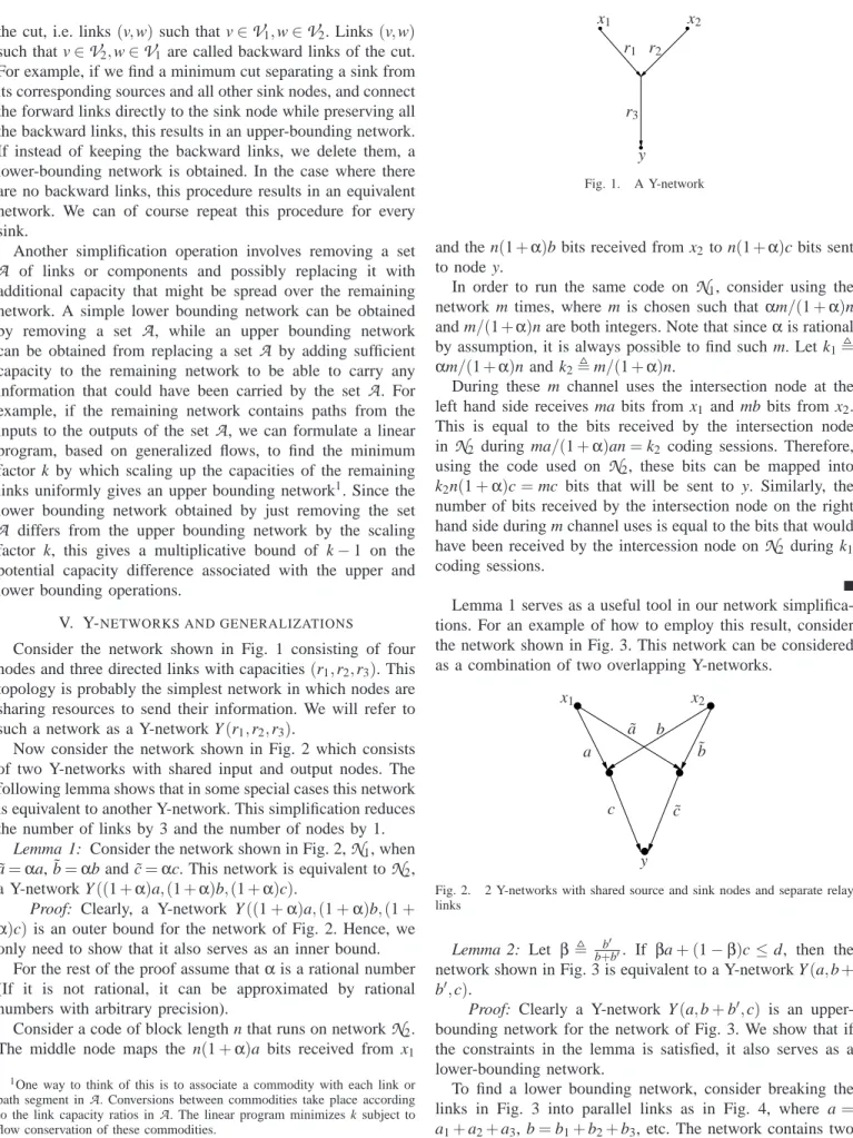
Consider the network shown in Fig. 1 consisting of four nodes and three directed links with capacities (r1,r2,r3). This topology is probably the simplest network in which nodes are sharing resources to send their information. We will refer to such a network as a Y-network Y(r1,r2,r3).

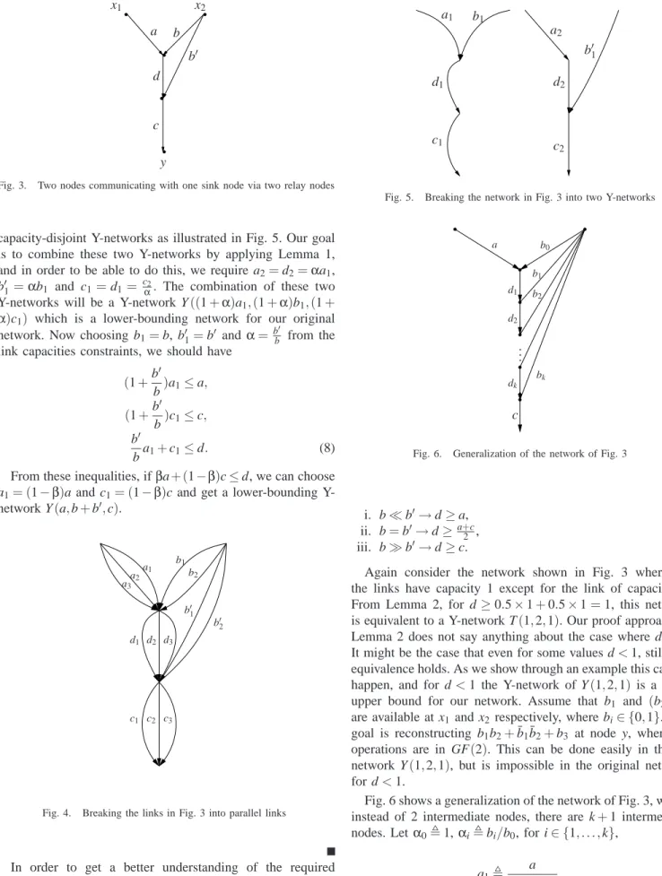
Now consider the network shown in Fig. 2 which consists of two Y-networks with shared input and output nodes. The following lemma shows that in some special cases this network is equivalent to another Y-network. This simplification reduces the number of links by 3 and the number of nodes by 1.

Lemma 1: Consider the network shown in Fig. 2,

N

1, when ˜

a=αa, ˜b=αb and ˜c=αc. This network is equivalent to

N

2, a Y-network Y((1+α)a,(1+α)b,(1+α)c).

Proof: Clearly, a Y-network Y((1+α)a,(1+α)b,(1+

α)c) is an outer bound for the network of Fig. 2. Hence, we only need to show that it also serves as an inner bound.

For the rest of the proof assume thatαis a rational number (If it is not rational, it can be approximated by rational numbers with arbitrary precision).

Consider a code of block length n that runs on network

N

2. The middle node maps the n(1+α)a bits received from x1

1_{One way to think of this is to associate a commodity with each link or}

path segment inA. Conversions between commodities take place according to the link capacity ratios inA. The linear program minimizes k subject to flow conservation of these commodities.

r1 r2

r3

x1 x2

y

Fig. 1. A Y-network

and the n(1+α)b bits received from x2 to n(1+α)c bits sent to node y.

In order to run the same code on

N

1, consider using the network m times, where m is chosen such that αm/(1+α)n

and m/(1+α)n are both integers. Note that sinceαis rational by assumption, it is always possible to find such m. Let k1, αm/(1+α)n and k2,m/(1+α)n.

During these m channel uses the intersection node at the left hand side receives ma bits from x1and mb bits from x2. This is equal to the bits received by the intersection node in

N

2 during ma/(1+α)an=k2 coding sessions. Therefore, using the code used on

N

2, these bits can be mapped into

k2n(1+α)c=mc bits that will be sent to y. Similarly, the number of bits received by the intersection node on the right hand side during m channel uses is equal to the bits that would have been received by the intercession node on

N

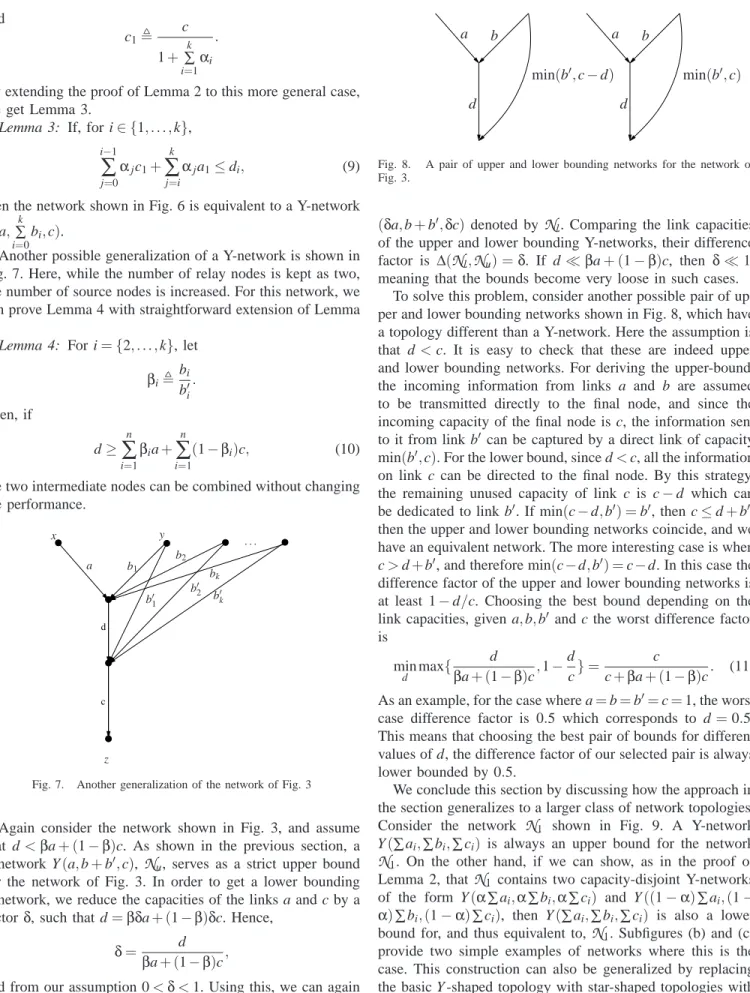
2during k1 coding sessions.

Lemma 1 serves as a useful tool in our network simplifica-tions. For an example of how to employ this result, consider the network shown in Fig. 3. This network can be considered as a combination of two overlapping Y-networks.

a ˜b b ˜ a c c˜ x1 x2 y

Fig. 2. 2 Y-networks with shared source and sink nodes and separate relay links

Lemma 2: Let β, _b+b′_b′. If βa+ (1−β)c≤d, then the network shown in Fig. 3 is equivalent to a Y-network Y(a,b+

b′,c).

Proof: Clearly a Y-network Y(a,b+b′,c) is an upper-bounding network for the network of Fig. 3. We show that if the constraints in the lemma is satisfied, it also serves as a lower-bounding network.

To find a lower bounding network, consider breaking the links in Fig. 3 into parallel links as in Fig. 4, where a=

PSfrag _{a b} b′ c d x1 x2 y

Fig. 3. Two nodes communicating with one sink node via two relay nodes

capacity-disjoint Y-networks as illustrated in Fig. 5. Our goal is to combine these two Y-networks by applying Lemma 1, and in order to be able to do this, we require a2=d2=αa1,

b′₁=αb1 and c1=d1= c_α2. The combination of these two Y-networks will be a Y-network Y((1+α)a1,(1+α)b1,(1+

α)c1) which is a lower-bounding network for our original network. Now choosing b1=b, b′1=b′ andα=b

′

b from the link capacities constraints, we should have

(1+b ′ b)a1≤a, (1+b ′ b)c1≤c, b′ ba1+c1≤d. (8)

From these inequalities, ifβa+ (1−β)c≤d, we can choose a1= (1−β)a and c1= (1−β)c and get a lower-bounding Y-network Y(a,b+b′,c). a1 a2 a3 b1 b2 b′ 1 b′ 2 c1 c2 c3 d1 d2 d3

Fig. 4. Breaking the links in Fig. 3 into parallel links

In order to get a better understanding of the required constraint stated in Lemma 2, consider the following special cases: a1 b1 c1 d1 a2 b′₁ c2 d2

Fig. 5. Breaking the network in Fig. 3 into two Y-networks

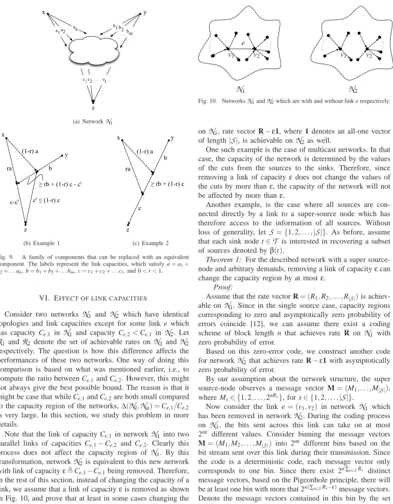
a b0 c d1 d2 dk b1 b2 bk .. .

Fig. 6. Generalization of the network of Fig. 3

i. b≪b′→d≥a,

ii. b=b′→d≥a+c

2 ,

iii. b≫b′→d≥c.

Again consider the network shown in Fig. 3 where all the links have capacity 1 except for the link of capacity d. From Lemma 2, for d≥0.5×1+0.5×1=1, this network is equivalent to a Y-network T(1,2,1). Our proof approach in Lemma 2 does not say anything about the case where d<1. It might be the case that even for some values d<1, still this equivalence holds. As we show through an example this cannot happen, and for d<1 the Y-network of Y(1,2,1) is a strict upper bound for our network. Assume that b1 and (b2,b3) are available at x1and x2respectively, where bi∈ {0,1}. The goal is reconstructing b1b2+¯b1¯b2+b3 at node y, where all operations are in GF(2). This can be done easily in the Y-network Y(1,2,1), but is impossible in the original network for d<1.

Fig. 6 shows a generalization of the network of Fig. 3, where instead of 2 intermediate nodes, there are k+1 intermediate nodes. Letα0,1,αi,bi/b0, for i∈ {1, . . . ,k},

a1, a 1+∑k i=1 αi ,

and c1, c 1+∑k i=1 αi .

By extending the proof of Lemma 2 to this more general case, we get Lemma 3.

Lemma 3: If, for i∈ {1, . . . ,k}, i−1

∑

j=0 αjc1+ k

∑

j=i αja1≤di, (9)

then the network shown in Fig. 6 is equivalent to a Y-network

Y(a,∑k i=0

bi,c).

Another possible generalization of a Y-network is shown in Fig. 7. Here, while the number of relay nodes is kept as two, the number of source nodes is increased. For this network, we can prove Lemma 4 with straightforward extension of Lemma 2.

Lemma 4: For i={2, . . . ,k}, let βi, bi b′_i. Then, if d≥ n

∑

i=1 βia+ n

∑

i=1 (1−βi)c, (10) the two intermediate nodes can be combined without changing the performance. d c x y z a b1 b′1 b2 b′₂ bk b′_k . . .

Fig. 7. Another generalization of the network of Fig. 3

Again consider the network shown in Fig. 3, and assume that d<βa+ (1−β)c. As shown in the previous section, a

Y-network Y(a,b+b′,c),

N

u, serves as a strict upper bound for the network of Fig. 3. In order to get a lower bounding Y-network, we reduce the capacities of the links a and c by a factorδ, such that d=βδa+ (1−β)δc. Hence,

δ=_β d

a+ (1−β)c,

and from our assumption 0<δ<1. Using this, we can again invoke Lemma 2 and get a lower-bounding Y-network of

a b d min(b′,c−d) a b d min(b′,c)

Fig. 8. A pair of upper and lower bounding networks for the network of

Fig. 3.

(δa,b+b′,δc) denoted by

N

_l. Comparing the link capacities of the upper and lower bounding Y-networks, their difference factor is ∆(

N

_l,

N

_u) =δ. If d ≪βa+ (1−β)c, then δ≪1, meaning that the bounds become very loose in such cases.

To solve this problem, consider another possible pair of up-per and lower bounding networks shown in Fig. 8, which have a topology different than a Y-network. Here the assumption is that d<c. It is easy to check that these are indeed upper

and lower bounding networks. For deriving the upper-bound, the incoming information from links a and b are assumed to be transmitted directly to the final node, and since the incoming capacity of the final node is c, the information sent to it from link b′ can be captured by a direct link of capacity min(b′,c). For the lower bound, since d<c, all the information

on link c can be directed to the final node. By this strategy, the remaining unused capacity of link c is c−d which can

be dedicated to link b′. If min(c−d,b′) =b′, then c≤d+b′, then the upper and lower bounding networks coincide, and we have an equivalent network. The more interesting case is when

c>d+b′, and therefore min(c−d,b′) =c−d. In this case the

difference factor of the upper and lower bounding networks is at least 1−d/c. Choosing the best bound depending on the

link capacities, given a,b,b′ and c the worst difference factor is min d max{ d βa+ (1−β)c,1− d c}= c c+βa+ (1−β)c. (11)

As an example, for the case where a=b=b′=c=1, the worst case difference factor is 0.5 which corresponds to d=0.5. This means that choosing the best pair of bounds for different values of d, the difference factor of our selected pair is always lower bounded by 0.5.

We conclude this section by discussing how the approach in the section generalizes to a larger class of network topologies. Consider the network

N

₁ shown in Fig. 9. A Y-network

Y(∑ai,∑bi,∑ci) is always an upper bound for the network

N

1. On the other hand, if we can show, as in the proof of

Lemma 2, that

N

1contains two capacity-disjoint Y-networks of the form Y(α∑ai,α∑bi,α∑ci) and Y((1−α)∑ai,(1− α)∑bi,(1−α)∑ci), then Y(∑ai,∑bi,∑ci) is also a lower bound for, and thus equivalent to,

N

1. Subfigures (b) and (c) provide two simple examples of networks where this is the case. This construction can also be generalized by replacing the basic Y -shaped topology with star-shaped topologies with arbitrary numbers of inputs and outputs.

an a1 bm c1c2 cl z x y . . . a2. . . b1 . . . b2 (a) NetworkN1 x y z c-c' c' ≤ (1-r) c b (1-r) a ra ≥ rb + (1-r) c - c' (b) Example 1 x y z c b (1-r) a ra ≥ rb + (1-r) c (c) Example 2

Fig. 9. A family of components that can be replaced with an equivalent

component. The labels represent the link capacities, which satisfy a=a1+

a2+. . .an, b=b1+b2+. . .bm, c=c1+c2+. . .cl, and 0<r<1.

VI. EFFECT OF LINK CAPACITIES

Consider two networks

N

1 and

N

2 which have identical topologies and link capacities except for some link e which has capacity Ce,1 in

N

1 and capacity Ce,2<Ce,1 in

N

2. Let

R

1 and

R

2 denote the set of achievable rates on

N

1 and

N

2 respectively. The question is how this difference affects the performances of these two networks. One way of doing this comparison is based on what was mentioned earlier, i.e., to compute the ratio between Ce,1and Ce,2. However, this might

not always give the best possible bound. The reason is that it might be case that while Ce,1and Ce,2are both small compared to the capacity region of the networks, ∆(

N

l,Nu) =Ce,1/Ce,2 is very large. In this section, we study this problem in more details.

Note that the link of capacity Ce,1in network

N

1 into two parallel links of capacities Ce,1−Ce,2 and Ce,2. Clearly this

process does not affect the capacity region of

N

1. By this transformation, network

N

2is equivalent to this new network with link of capacityε_,Ce,1−Ce,1being removed. Therefore, in the rest of this section, instead of changing the capacity of a link, we assume that a link of capacityεis removed as shown in Fig. 10, and prove that at least in some cases changing the capacity of a link by εcannot have an effect larger thanεon the set of achievable rates, i.e., if the rate vector R is achievable

N

1

N

2

e

v1

v1 v2 v2

Fig. 10. NetworksN1andN2which are with and without link e respectively.

on

N

1, rate vector R−ε1, where 1 denotes an all-one vector of length|S|, is achievable on

N

2 as well.

One such example is the case of multicast networks. In that case, the capacity of the network is determined by the values of the cuts from the sources to the sinks. Therefore, since removing a link of capacity εdoes not change the values of the cuts by more thanε, the capacity of the network will not be affected by more thanε.

Another example, is the case where all sources are con-nected directly by a link to a super-source node which has therefore access to the information of all sources. Without loss of generality, let

S

={1,2, . . . ,|S|}. As before, assume that each sink node t∈

T

is interested in recovering a subset of sources denoted byβ(t).

Theorem 1: For the described network with a super

source-node and arbitrary demands, removing a link of capacityεcan change the capacity region by at mostε.

Proof:

Assume that the rate vector R= (R1,R2, . . . ,R_|S|)is achiev-able on

N

1. Since in the single source case, capacity regions corresponding to zero and asymptotically zero probability of errors coincide [12], we can assume there exist a coding scheme of block length n that achieves rate R on

N

₁ with zero probability of error.

Based on this zero-error code, we construct another code for network

N

2 that achieves rate R−ε1 with asymptotically zero probability of error.

By our assumption about the network structure, the super source-node observes a message vector M= (M1, . . . ,M_|S|), where Ms∈ {1,2, . . . ,2nRs}, for s∈ {1,2, . . . ,|

S

|}.

Now consider the link e= (v1,v2) in network

N

1 which has been removed in network

N

₂. During the coding process on

N

₁, the bits sent across this link can take on at most 2nε different values. Consider binning the message vectors

M= (M1,M2, . . . ,M|S|) into 2nε different bins based on the

bit stream sent over this link during their transmission. Since the code is a deterministic code, each message vector only corresponds to one bin. Since there exist 2n∑s∈SRs _distinct

message vectors, based on the Pigeonhole principle, there will be at least one bin with more that 2n(∑s∈SRs−ε)_{message vectors.}

Denote the message vectors contained in this bin by the set

M

0.

Therefore, in order to run the code for

N

₁on network

N

₂, we need to specify the assumption of node v2 about the message that it would have received from node v1in

N

1. Let node v2 assume that it always receives the bit pattern corresponding to the bin containing

M

0. Making this assumption and having the rest of

N

2to perform as in

N

1, it is clear that all message vectors in

M

0can be delivered with zero probability of error on

N

2as well. In other words, if the input to the super source node in

N

2 is one of the message vectors in

M

0, then each sink t∈

T

recovers its intended message M_β(t)with probability one. In the rest of the proof we show how this set

M

0can be used to deliver independent information to different receivers over network

N

2.

Define random vector U = (U1,U2, . . . ,U_|S|) to have a uniform distribution over the elements of

M

0. For each input vector U, each sink node t, recovers U_β(t) perfectly.

The described model with input U, and ouputs U_β(t), for

t ∈

T

is a deterministic broadcast channel (DBC)2 whose capacity region is known. Therefore, we can employ this DBC to deliver information on

N

2.

Before doing this, we slightly change the set of sink nodes, and replace the set of sinks

T

by

T

e as described in the following. This modification does not affect the functionality of the network, but simplifies the statement of the proof. Divide each sink node t into|β(t)|sink nodes, such that each one has access to all the information available to the node t, but is only interested in reconstructing one of the sources. Let

T

_e denote this expanded set of sinks. Consider a subset

T

_sof size|

S

|of

T

e such that each source s∈

S

is recovered by one of the sinks in

T

S. Since each sink in

T

s only recovers one source, hence there should be a one-to-one correspondence between the elements of

S

and

T

s.

Now consider the DBC with input U and outputs{Ut}t∈Ts.

Since the code is zero-error, and there is a one-to-one cor-respondence between the elements of

S

and

T

s, {Us}s∈S can be replaced by {Us}s∈S. The capacity region of this DBC, as explained in Appendix A, can be described by the set of rates (r1,r2, . . . ,r_|S|)satisfying

∑

s∈A

rs≤H(UA), (12)

for all

A

⊂

S

. From our construction,

H(US) =H(U1,U2, . . . ,U|S|) n(

∑

s∈S

Rs−ε). (13)

On the other hand, for each

A

⊂

S

H(US) =H(UA) +H(US\A). (14)

2_{DBCs and their capacity regions are briefly described in Appendix A.}

Therefore, H(U_A) =H(U_S)−H(U_S\A) ≥n(

∑

s∈S Rs−ε)−

∑

s∈S\A H(Us) ≥n(

∑

s∈S Rs−ε)−

∑

s∈S\A nRs =n(

∑

s∈A Rs−ε). (15)

It is easy to check that the point(r1,r2, . . . ,r_|S|) =n(R−ε1)

satisfies all inequalities required by (12). Hence, using the network

N

₂as a DBC, the rate vector R−εcan be transmitted to nodes in

T

s.

We now argue that the described DBC code, with no extra effort, delivers the rate vector R−εon network

N

₂to all sinks, not just those in

T

_s. The reason is that for each message vector

M∈

M

0, and consequently for each input U, all sink nodes in

T

ethat are interested in recovering a source s, i.e., for all t∈

T

e such thatβ(t) =s, receive Ms with probability one. Hence, if by the described coding scheme rate Rsis delivered to one of them, then the rest are able to receive the same data stream at rate Rs as well.

For some simple cases of multi-source multi-demand case networks, for instance when the link of capacity εis directly connected to one of the sources, the same result still holds, i.e. removing that link cannot change the capacity region by more than ε. However, for the general case, it remains open as to how much removing a link of capacityεcan affect the capacity region of the network.

VII. CYCLES AND DELAYS

In [13], the capacity of a channel is defined in terms of bits per channel use. In the case where there are no cycles, this definition is equivalent to defining capacity in terms of bits transmitted per unit time. However, we do not know whether in a general network with cycles and delays, these two definitions, i.e., bits per channel use versus bits per unit time, could result in different capacity regions. For example, consider two networks

N

1 and

N

2 that are identical except for a single component cycle, illustrated in Fig. 11. In

N

2the transmission delay from v1to v2is larger than in

N

1due to the added node v0, assuming that each link introduces unit delay. Now, we do not know whether achieving capacity on

N

₁could require interactive communication over a feedback loop, where each successive symbol transmitted by v1depends on previous symbols received from v2 and vice versa. If we try to run the same code on

N

2, the number of symbols per unit time that can be exchanged by nodes v1 and v2 is decreased because of the additional delay introduced by node v0. Hence, if the rate is defined in terms of bits communicated per unit time, this additional delay will reduce the capacity region. However, if the capacity is defined in terms of bits communicated per channel use, by letting each node wait until it has received the information it requires to generate its next symbol, the

replacements v1 v2 (a) Component ofN1 v1 v2 v0 (b) Component ofN2

Fig. 11. Changing the delay between two nodes by introducing an extra

node

delivered rates and consequently the capacity region will not be affected.3

In most of the operations introduced in this paper, the number of hops between nodes is different in the original network compared to its simplified version. Therefore, such operations in a cyclic graph with delay can potentially change the capacity region in ways that are not predicted by our analysis. Hence, in this paper we have restricted ourselves to the case of acyclic graphs. However, studying the effect of these operations in a general network with cycles remains as a question for further study.

VIII. CONCLUSIONS

In this paper, we proposed new techniques for efficiently approximating or bounding the capacity of networks with complex topologies and arbitrary communication demands, such as non-multicast and functional demands. We proposed to take a new approach based on systematic graph operations that can be applied recursively to simplify large networks, so as to facilitate the application of computational bounding tools. Besides its generality, another motivation for such a recursive graph-based approach is that it lends itself to tractable “divide-and-conquer” algorithms for analyzing very large networks and allows computation to be traded off against tightness of obtained bounds according to the extent of simplification.

Techniques proposed for networks of directed noiseless point-to-point links (bit pipes) can be readily applied to networks of noisy multi-terminal channels by using the results of Koetter et al. [9] to replace each noisy link with a bounding model consisting of such bit pipes. However, it may be possible to obtain better bounds by developing simplification tools that are directly applicable to noisy networks. Thus, we will seek to extend the above work to networks containing noisy broadcast, multiple access and interference links.

APPENDIX A

DETERMINISTIC BROADCAST CHANNEL

Deterministic broadcast channels (DBC) are spacial cases of general broadcast channels. In a K-user DBC,

P((Y1, . . . ,YK) = (y1, . . . ,yK)|X=x)∈ {0,1}.

In other words, since in a BC the capacity region only depends on the marginal distributions [13], a K-user DBC can be

3_{Note that in the case of multicast, since it is known that capacity-achieving}

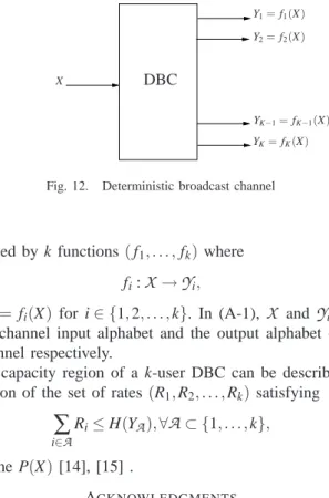
codes do not require such communication over feedback loops, the capacity region remains unchanged under both definitions, even in the case of cyclic graphs. X Y1=f1(X) Y2=f2(X) YK−1=fK−1(X) YK=fK(X) DBC

Fig. 12. Deterministic broadcast channel

described by k functions (f1, . . . ,fk)where

fi:

X

→

Y

i, (A-1)

and Yi= fi(X) for i∈ {1,2, . . . ,k}. In (A-1),

X

and

Y

i refer to the channel input alphabet and the output alphabet of the

ith channel respectively.

The capacity region of a k-user DBC can be described by the union of the set of rates(R1,R2, . . . ,Rk)satisfying

∑

i∈A

Ri≤H(YA),∀A⊂ {1, . . . ,k}, (A-2) for some P(X)[14], [15] .

ACKNOWLEDGMENTS

This work has been supported in part by the Air Force Office of Scientific Research under grant FA9550-10-1-0166 and Caltech’s Lee Center for Advanced Networking.

REFERENCES

[1] Kramer. G. and S. Savari. Capacity bounds for relay networks. In Proc. 2006 Workshop Inf. Theory Appl., La Jolla, CA, feb 2006.

[2] M. Adler, N. J. Harvery, K. Jain, R. Kleinberg, and A. R. Lehman. On the capacity of information networks. In SODA, 2006.

[3] N. J. A. Harvey, R. Kleinberg, C. Nair, and Y. Wu. A “chicken and egg” network coding problem. In Proc. IEEE Int. Symp. Inform. Theory, Nice, France, June 2007.

[4] R.W. Yeung. A framework for linear information inequalities. Informa-tion Theory, IEEE TransacInforma-tions on, 43(6):1924 –1934, nov. 1997. [5] A.T. Subramanian and A. Thangaraj. A simple algebraic formulation

for the scalar linear network coding problem. ArXiv e-prints, July 2008. [6] Xitip - information theoretic inequalities prover. http://xitip.epfl.ch/. [7] M. M´edard and R. Koetter. An algebraic approach to network coding.

IEEE/ACM Transactions on Networking, pages 782–795, 2003. [8] T. H. Chan. Capacity regions for linear and abelian network code. In

NETCOD, San Diego, CA, January 2007.

[9] R. Koetter, M. Effros, and M. M´edard. A theory of network equivalence, parts i and ii. ArXiv e-prints, July 2010.

[10] R. W. Yeung. Information Theory and Network Coding. Springer, 2008. [11] M. Effros. On capacity outer bounds for a simple family of wireless networks. In Information Theory and Applications Workshop, San Diego, CA, 2010.

[12] T. Chan and A. Grant. On capacity regions of non-multicast networks. In Proc. IEEE Int. Symp. Inform. Theory, Austin, TX, June 2010. [13] T. Cover and J. Thomas. Elements of Information Theory. Wiley, New

York, 2nd edition, 2006.

[14] K. Marton. The capacity region of deterministic broadcast channels. In Proc. IEEE Int. Symp. Inform. Theory, Paris-Cachan, France, 1977. [15] M. S. Pinsker. Capacity of noiseless broadcast channels. Probl. Inform.