NOTE: These materials were prepared by subcontractors for consideration by the

(1)

NOTE:

These materials were prepared by subcontractors for consideration

by the

Committee on Geographic Variation in Health Care Spending

and Promotion of High-value Care

. These analyses were

commissioned and overseen by the Committee. However, the

findings and views expressed in the subcontractor reports do not

necessarily reflect those of the NRC/IOM or the Committee.

Neither the methodology nor the subcontractor reports have been

subject to formal institutional review for the Interim Report. As the

committee continues to review the findings from the analyses

contained herein, we invite you to provide feedback on the content of

these reports. Please note that any comments will be entered into the

project’s public access file, and will be available for public review.

(2)

Geographic Variation in Health Care

Spending and Promotion of High-Value Care

Final Report

(3)

Executive Summary

After the passage of the Affordable Care Act in 2010, the U.S. Secretary of Health and Human Services asked the Institute of Medicine to undertake a study on geographic variation in health care spending, utilization, and quality. The end goal of this study is to explore whether there are clear drivers of variation both within and across different health care populations. To answer that charge, the IOM commissioned this report as well as four additional population-specific studies of variation in health care outcomes. This report synthesizes those earlier studies and analyzes a measure of total population health care spending to respond to an additional set of research questions.

In synthesizing the population-specific studies of geographic variation in health care spending, utilization, and quality, this report finds that:

• _{Across the populations, variation in spending, utilization, and quality is high.}

Coefficients of variation on prescription drug utilization, for example, range from 0.13 to 0.62, while standard deviations of quality outcomes are as high as 0.52. While some populations vary more than others, geographic variation exists in all populations.

• _{Without adjusting for any predictors, coefficients of variation on input price}

adjusted spending range from 0.12 to 0.59. Common predictors of variation like health status and health care market characteristics reduce this variation across the populations. However, the majority of that variation remains even after adjusting for those predictors.

• _{Regionally-based policies would likely have a lesser impact on geographic variation}

if they are implemented at more aggregated levels of geography. About half of the variation in health care spending and utilization is occurring at sub-regional levels of geography. This result is particularly true for spending in the commercially insured population.

In analyzing how a measure of total (all-population) spending varies geographically and how well it predicts health care quality in the Medicare population, this report finds:

• _{Total spending varies geographically at a similar magnitude as the}

population-specific studies. It is generally more variable than commercial spending but less variable that Medicaid spending.

• _{Adjusting for important predictors of health care variation reduces the coefficient}

of variation of the measure of total spending. In particular, adjusting for health status redues variation by 25%, and adjusting for health status as well as market factors reduces variation by 30% overall. These reductions in variation are of a similar magnitude as those in the population-specific studies.

(6)

• _{Total spending is a somewhat worse predictor of Medicare quality than is Medicare}

spending, but the differences are modest. In addition, Medicare spending improves some measures of quality, but increased total spending only reduces the quality of care.

(7)

Introduction

Why Study Geographic Variation?

After the passage of the Affordable Care Act in 2010, the U.S. Secretary of Health and Human Services asked the Institute of Medicine to undertake a study on geographic variation in health care spending, utilization, and quality. (Institute of Medicine 2012) The end goal of this study is to explore whether there are clear drivers of variation both within and across different health care populations. The particular populations of interest are the privately / commercially insured, Medicare beneficiaries, Medicaid beneficiaries, and the uninsured. The IOM, then, will use the data and analysis gathered during this project to present recommendations to the Department of Health and Human Services on whether and how Medicare policies can be altered to promote higher-value care, perhaps through the use of a value index. (Institute of Medicine 2012)

In addition to the policy relevance of the project, a major reason to study geographic variation in health care spending is to confirm the findings of existing studies and extend the literature to cover additional populations. Guided by the pivotal work of the Dartmouth Atlas of Health Care, there is strong, well-supported evidence of substantial geographic variation in spending, utilization, quality, and health care outcomes for the Medicare population. (Skinner 2011) (Newbergh) While more recent studies have attempted to extend the literature on geographic variation beyond Medicare, the evidence remains limited. (Philipson et al. 2010) (Chernew et al. 2010) Therefore, the IOM’s study is important for its contribution to knowledge about variation in a number of different populations.

Overview of the Project

To operationalize their study of geographic variation in health care within and across populations, the IOM commissioned studies that each focus on a particular payer population. Each study, or population, is based on various outcome measures of spending, utilization, and quality as well as plausible predictors of variation. Those measures are used to explore the scope of and explanations for geographic variation in health care. To come to their final results, the studies rely on ordinary least squares (OLS) regressions to calculate the degree of variation in health spending and to test explanations of variation. Finally, the findings from those studies and additional data on other populations are combined to create a measure of total spending by geographic region where similar explanations of variation are tested.

Populations and Payers

The four population-specific studies focus on fee-for-service Medicare, fee-for-service Medicaid, and the commercially insured population from 2007 to 2009. PHE’s study adds

(8)

to those populations by including the uninsured and Medicare and Medicaid managed care in its estimate of the total population and combines the full set of these populations into a measure of total spending. Specifically, the Medicare study evaluates health care spending, utilization, and quality for the population of beneficiaries enrolled in fee-for-service Medicare, but not Medicare Advantage. It tracks Part D claims for the fee-for-service beneficiaries enrolled in Medicare Part D, in addition to claims from Parts A and B. The Medicaid study focuses on beneficiaries with fee-for-service Medicaid and Medicaid managed care enrollees with Primary Care Case Management managed care (known as “partial” managed care). The two studies of the commercially-insured population rely on different sources for claims data and slightly different populations. The MarketScan study analyzes the aged 0 to 64 population whose claims are tracked in Thomson Reuter’s MarketScan Commercial Claims and Encounters Database. The OptumInsight study, on the other hand, includes data on enrollees and dependents aged 0 to 85, tracked by OptumInsight.

Each of these studies analyzes geographic variation in health care spending, utilization, and quality for these populations.

Definitions of Geography

All the studies evaluate geographic variation in health care spending, utilization, and quality, at three levels of geography: Hospital Referral Regions (HRRs), Hospital Service Areas (HSAs), and Metropolitan Statistical Areas (MSAs). HRRs and HSAs were developed and defined by the research team responsible for the Dartmouth Atlas and are tied to the enrollee’s zip code. Both measures are based on the use of health resources and referral patterns. Importantly, HSAs are perfectly nested within HRRs. (2012) MSA’s are based on population centers as defined by the Census Bureau and are not necessarily geographically related to either HRRs or HSAs. (U.S. Census 2012) All of the analyses were performed at the HRR, HSA, and MSA level. Most results will focus on the HRR level.

Outcome Measures

The basic unit of spending utilized in the various studies is per member per month (PMPM) total spending. This measure is defined as the sum of all spending on an enrollee for health care in an average month (in 2009 dollars). In addition to total per member per month spending, the studies also all look at the variation in input price adjusted spending. To do so, inpatient claims are adjusted using the Hospital Wage Index for the enrollee’s county. Outpatient services and inpatient profession services are adjusted using a combination of the Relative Value Unit weight and the Geographic Practice Cost Index. Drug and durable medical equipment spending is not adjusted. Some studies use additional adjustment factors as a supplement. This analysis will focus on input price adjusted spending.

The studies all evaluate utilization of health services through five shared measures: inpatient admissions, emergency department visits, outpatient visits, prescription drug fills, and imaging procedures. In general, these outcomes are measured as counts of days

(9)

with one of these types of visits with a maximum of one visit per day. Prescription drug fills are standardized to a 30-day supply. In addition to these utilization counts, the studies include additional measures that are unique to their methodology or are only shared with another study. Finally, all studies report two measures of health care quality—Patient Safety (PSI) and Prevention Quality (PQI). Both measures are modeled after, but may not perfectly compare with, measures from the Agency for Healthcare Research and Quality (AHRQ). They are composites of individual measures of safety and prevention.

Predictors of Variation

Based on the existing literature exploring the question of what predictors account for the variation in health care spending, utilization, and quality (e.g., health status, market-specific variables), the studies include various predictors of geographic variation. (Zuckerman et al. 2010) (Sutherland, Fisher, and Skinner 2009) (Fisher et al. 2003) These include individual age and sex (as well as their interaction), race or ethnicity, income, patient health status (using a claims-based measure of health status), the percent of the year a patient is enrolled, and predictors based on the local health care market. While some predictors are defined slightly differently across studies, these are the common explanations of variation. Each study had additional, unique predictors of variation relevant to their populations.

Methods of Population-Specific Studies

In order to estimate the magnitude of geographic variation in health care spending, the studies regress their spending, utilization, and quality measures against these predictors of variation. Those outcomes are then tested and analyzed to determine the extent of variation.

In order to measure the explanatory power of individual predictors, the studies all perform series of regressions on the outcome variable of input price adjusted spending. First a “control” regression is performed that included only year and partial year enrollment. Then, additional predictors are added. The resulting “clusters” of predictors are compared to see whether adding predictors explained additional geographic variation. There were 10 clusters in total, see Table 4 for a complete table of these clusters of predictors.

Research Questions

PHE was tasked with two distinct pieces of analysis: synthesizing the existing data created by these studies and aggregating the population-specific results with data on additional populations to estimate total spending by HRR. Each portion of the analysis has a set of narrower research questions. The first portion of the analysis, the synthesis, aims to answer a few key questions:

1. Across the studies, how do spending, utilization and quality vary within and between areas (such as HRRs)?

(10)

2. How much variation is explained by observed predictors? Are the explanations consistent across different payers and populations?

3. At what level(s) of geography is the variation occurring?

The second portion of the analysis is executed to answer the following research questions: 4. How does “total” spending – including commercial, Medicare, Medicaid, and the

uninsured – vary across regions? 5. What predictors explain this variation?

6. Is total spending or Medicare-only spending a better predictor of Medicare quality outcomes?

Background on Subcontractor Data

Populations & Databases

The MarketScan study relies primarily on data from 2005 to 2010 from Thomson Reuters MarketScan Commercial Claims and Encounters Database. This data comes from either private health plans or employers and covers employees and their dependent family members. For each enrollee, the database includes the dates and location of inpatient and outpatient claims, spending incurred by those claims and, for 80 percent of the sample, pharmaceutical claim dates and spending. For the remaining 20 percent of the sample, the MarketScan study predicts likely pharmaceutical use and expenditures. It additionally contains relevant demographic data (age, gender) as well as insurance plan details, enrollment, and out of pocket spending. The analysis focuses specifically on claims occurring during 2007, 2008, and 2009. To supplement demographic data not included in the MarketScan database, this study relies on U.S. Census Bureau data at either the zip-code or county level for measures of race and income. As is the case with all private health insurance claims data, MarketScan is not designed to be representative of the privately insured US population. This fact may affect generalizability to the entire privately insured population, although its sheer size suggests that important information can be gleaned. As noted above, the OptumInsight study uses data tracked by OptumInsight’s Normative Health Information Database on commercially insured individuals aged 0 to 85. The data includes information from claim years 2006 to 2010 from both private, commercially insured plans (PCIs) and Employer group health plans (EGHPs). These claims represent about 23 million covered lives. The data are collected from various health care sites including inpatient, outpatient, emergency room and more. Claims contain dates, codes for services rendered, as well as billing amounts. In addition to claims data, the database contains relevant demographic information like age, sex, race/ethnicity, and income.

(11)

Importantly, about 6 million members do not have data on claims for pharmacy coverage which likely leads to an undercount of spending and prescription drug fills. Also, claims for long-term care and institutional care are not included. (The Lewin Group 2012) As with the MarketScan data, the OptumInsight database is not designed to be nationally representative, and similar caveats apply regarding generalizability.

The Medicare study, which includes the over 65 population and individuals under 65 who are eligible for Medicare, utilizes the universe of Medicare claims from 2005 to 2010 for its analysis. In particular, the study uses Medicare Parts A, B, and D claims files which are episodic and record all interactions between Medicare beneficiaries and providers who are paid by Medicare. The data show the services provided, the date, the cost of those services, who provided the services, and important demographic information about the individual seeking care. The claims files are separated by the types of claims (prescription drugs versus inpatient, etc.), but the study includes all relevant claim types in this analysis. Those claims files are also matched to Parts A, B, C, and D enrollment data which contains information on demographics, months of enrollment in the different programs, any third-party buyer information, and enrollment in managed care. The Medicare data exclude the Medicare Advantage (i.e., Medicare HMO) population, which has been rising over time as a proportion of total Medicare beneficiaries. Currently, Medicare Advantage patients comprise nearly 25% of the total Medicare population.(Kaiser Family Foundation 2011) A variety of existing literature finds differences between the Medicare Advantage and Medicare fee-for-service populations, in terms of service utilization, and baseline health status. (Batata 2004) This suggests caution is again warranted in extrapolating from the study results to the entire Medicare program.

The Medicaid study focuses on the set of Medicaid beneficiaries who are enrolled in fee-for-service Medicaid. In order to identify those individuals and their spending, utilization, and quality of care, the study uses the universe of Medicaid claims in the Medicaid Statistical Information System (MSIS) for 2005 to 2010. This data has quarterly files with paid claims, any adjustments, and enrollment information. These files are broken into eligibility, inpatient hospital claims, long-term care claims, other services/therapy, and prescription drugs. A drawback of this data is that not all states use standardized systems for reporting claim or procedure codes. Additionally, many enrollees are covered under multiple plans and programs that are not uniformly reported to the MSIS system. Therefore, these data were far more complex and subject to even more limitations than the data used in the other studies.

In part because of the complicated nature of the Medicaid study data and in part because of the unreliable nature of capitated claims data, almost all Medicare Managed Care enrollees are excluded from the study. The Medicaid Managed Care Population represents more than half of Medicaid beneficiaries. (The Kaiser Family Foundation 2012) Managed care enrollees are kept only if they are enrolled in “partial” managed care. Partial managed care refers to the fact that only some, ancillary services are covered separately from the fee-for-service program, or that physicians are paid a small fee to actively manage the care of these

(12)

beneficiaries. In addition, those beneficiaries who do not have coverage for the full set of services are excluded. As a result of this exclusion, the study results may not generalize to the total Medicaid population.

Methods

The MarketScan study estimated mean outcome measures (PMPM spending, utilization, quality, etc.), or area effects, by first fitting an OLS regression without area fixed effects, and then computing area effects as the mean regression residuals within each area. In adjusting outcomes, independent variables were mean-centered using the population mean. In the MarketScan analysis, estimates of average residuals and area effects from conventional fixed effects regressions had a greater than +0.98 correlation, yet the average residuals approach was computationally more efficient. (Chernew et al. 2012) The MarketScan study also employed a Bayesian shrinkage factor to control for the fact that small samples have less reliable spending estimates.1

The OptumInsight study generated area level estimates using conventional fixed-effects regressions. As with the MarketScan study, key independent variables were mean-centered according to the national level mean to predict adjusted mean area effects. Many of these estimates, particularly those related to spending, were additionally normalized for reasons of data privacy and security. The normalizing scalar, spending by a national average sample person, was derived from the 2009 Medical Expenditure Panel Survey (MEPS). The OptumInsight study did not perform any additional procedures to control for the size of geographic region or the reliability of the estimates.

The fee-for-service Medicare and Medicaid analyses generated mean area effects by fitting an OLS regression without fixed effects and estimating the area effects as the average of the individual residuals. This method was nearly identical to MarketScan’s. Where it differed was that it did not shrink its estimates based on geography and it did not mean center independent variables with the population mean. Instead, mean area effects were adjusted by adding the average of the individual residuals in a given region to the average value of the outcome variable being analyzed across all regions. The Medicare and Medicaid studies did not perform additional sensitivity tests like MarketScan, but based on MarketScan’s findings, utilizing the average of residuals should yield similar results to implementing fixed effects regressions.

The mean outcome measures mentioned above were also standardized across the four population specific studies. Each study estimated area effects for total spending, input price adjusted spending, five shared measures of utilization, and two shared measures of quality. In addition, the area effects for input price adjusted spending were estimated after controlling for a series of iterative “clusters” of predictors. In total, input price adjusted

1_{In practice, the Bayesian shrinkage factor was very small and did not qualitatively impact the results of the}

(13)

spending was estimated for 10 of these clusters. Clusters 1 through 6 and Cluster 10 included predictors of demographic, health status, and health plan measures. Clusters 7 through 9, or the “market clusters,” included estimates of the local health market along with various demographic, health status, etc. predictors. In their analyses, the studies treated the market clusters differently than the non-market clusters

In particular, in an effort to standardize the findings of the four studies regarding the measurement of the impact of market variables on variation in input price adjusted health spending, the IOM asked the studies to perform a two-stage regression. In the first stage, the studies performed their original OLS regressions using either fixed effects or not. In the second stage, those first-stage estimates of area effects were regressed against different sets of market predictors. However, only the MarketScan study, Medicare, and Medicaid studies utilized the same collections of market predictors, so they can be compared directly.

As noted, the four studies generated estimates of quality measures. OptumInsight performed logistic regressions on some of the cluster predictors (age, sex, year and health status) for the PSIs and PQIs, predicted the probability of the outcomes at an individual level, and then averaged at the area level to produce a rate. Because logistic regression does not produce residuals as OLS does, it is not clear how adjustment for age, etc., was implemented. In any event, the analysis reportedly risk adjusted based on covariates from the cluster regressions, rather than the covariates used in the AHRQ measures themselves. (The Lewin Group 2012) MarketScan used logistic models for “rare” quality outcomes; otherwise, linear probability models were used. MarketScan explicitly noted that its rate is risk-adjusted by multiplying the ratio of observed-to-expected outcomes by a reference rate. The Medicare and Medicaid studies may have implemented the PSI, PQI and Inpatient Quality Indicator (IQI) composites by risk adjusting based on the AHRQ covariates. It appears that at least the PSI and IQI composites were reported as observed-to-expected ratios. Thus, while correlations across studies could be assessed, mean levels and variation are not directly comparable across some payer populations.

Assessment of Studies of Commercially Insured

The two studies of the commercially insured merited comparison. There was a difference in population (OptumInsight included 65-to-85 year olds.) There were also differences in methods, for example, conventional fixed effects at the area level with OptumInsight, versus residuals averaged by area for MarketScan. MarketScan explored the importance of fixed effects versus area residuals in its own population, and found that the resulting area effects had a very high correlation (in excess of 0.98). MarketScan also applied a Bayesian shrinkage factor, and found that its effect was minimal.

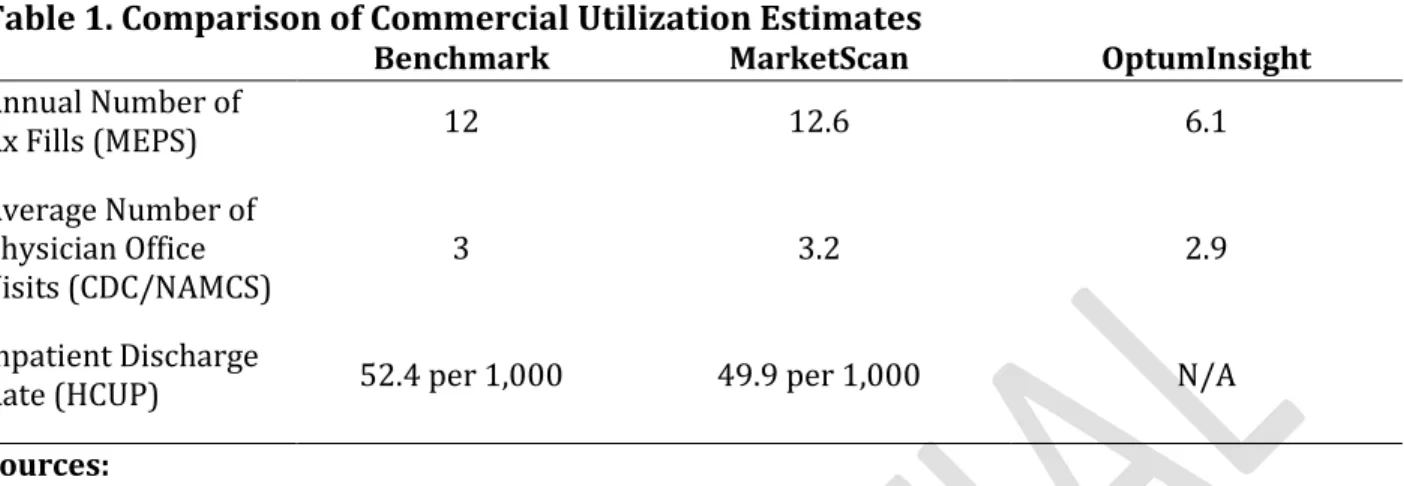
To further assess the commercial studies, outside estimates of utilization by the privately insured population were compared as benchmarks. These national benchmarks came from sources like the Centers for Disease Control, MEPS, etc. The comparisons are shown in Table 1 below.

(14)

Table 1. Comparison of Commercial Utilization Estimates

Benchmark MarketScan OptumInsight

Annual Number of Rx Fills (MEPS) 12 12.6 6.1 Average Number of Physician Office Visits (CDC/NAMCS) 3 3.2 2.9 Inpatient Discharge

Rate (HCUP) 52.4 per 1,000 49.9 per 1,000 N/A

Sources:

MEPS: http://meps.ahrq.gov/mepsweb/data_files/publications/st245/stat245.pdf CDC (based on data from NAMCS): http://www.cdc.gov/nchs/data/databriefs/db41.PDF HCUP: Analysis performed by MarketScan study, results available in their Final Report

Because these are representative, national benchmarks, PHE determined that MarketScan’s data was more reliable as they adhere more closely to these benchmarks. Additionally, since the spending estimates were quite similar, differences in utilization benchmarks were the best available determinant of the quality of the results. Given these findings, in the analysis of total spending, PHE relied on the MarketScan findings. But, for complete reporting, OptumInsight’s results are reported alongside other study-specific results.

Findings of Analysis

In an effort to synthesize the population-specific study results (research questions 1 through 3), PHE compared the findings of the individual subcontractors. In general, substantial variation existed, and continued to exist even after successive clusters of predictors were included; outcome measures were not highly correlated across payers, and a sizeable share of the variation was occurring at lower levels of geography than the HRR. In addition, it is possible that variation occurs at even lower levels – even across individual providers and hospitals – than can be detected using the data sources available in this project. (Doyle Jr, Ewer, and Wagner 2010) (Bradford et al. 2001) The spending, utilization, and quality measures reported and analyzed, reflect the total health care use (rather than disease-specific use) by all individuals in the different payer populations.

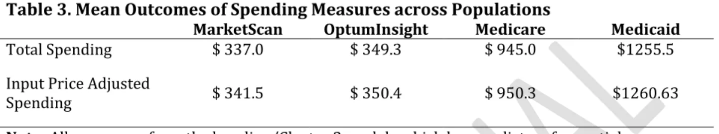
Spending

Estimates of mean unweighted spending were similar for the two commercial subcontractors, with OptumInsight coming in slightly higher than MarketScan (which was

(15)

not surprising, given their relatively older population). As shown in Table 3, Medicare and Medicaid had substantially higher estimates of average spending—between three and four times as large as the commercial populations, respectively.

Table 3. Mean Outcomes of Spending Measures across Populations

MarketScan OptumInsight Medicare Medicaid

Total Spending $ 337.0 $ 349.3 $ 945.0 $1255.5

Input Price Adjusted

Spending $ 341.5 $ 350.4 $ 950.3 $1260.63

Note: All means are from the baseline/Cluster 2 models which has predictors for partial-year enrollment, age, age*sex, year, and health status.

As noted earlier, the IOM emphasized the role of input price-adjusted spending in its

guidance to the studies. The 10 clusters of predictors are described in Table 4. For example, cluster 1 adds age, sex and their interaction to the minimal adjustment of the “control” cluster (which accounted for year and partial year enrollment, as operationalized in each study.)

Table 4. Clusters of Predictors Used in Regressions

Cluster Included Predictors Additional Notes

Control Year, Partial Year Enrollment (PYE) All Studies

1 Control + Age, Sex, Age*Sex All Studies

2 (“Baseline”) Cluster 1 + Health Status All Studies

3 Cluster 1 + Race All Studies

4 Cluster 1 + Income Medicaid’s Cluster 4 was

identical to Cluster 1 as they do not have a predictor for income

5 Cluster 2 + Race, Income All Studies

6 Cluster 1 + Benefit Generosity, Plan Type, Plan

Size MarketScan & OptumInsight Only

7 Cluster 1 + Market Variables Market Analysis Only (2 Stage)

8 Cluster 6 + Health + Market Variables (MarketScan)

Cluster 5 + Market Variables + More Market

Market Analysis Only (2 Stage) Additional Variables: Nurses per capita, dual eligible, payer

(16)

Variables (Medicare & Medicaid) mix

9 Cluster 5 + Market Variables Market Analysis Only (2 Stage)

10 Cluster 5 + Dual Eligible, Supplemental Coverage (Medicare), Institutionalization, State Dummies (Medicaid)

Medicare and Medicaid Only Note: Market Variables are: Total Population, PCPs per 1,000, Specialists per 1,000, Beds per 1,000, % HMO, % PPO, % POS, % Uninsured, Primary Care Shortage Area, Malpractice GPCI, HHI Bed, Teaching Hospital, Government Hospital, Specialty Hospital

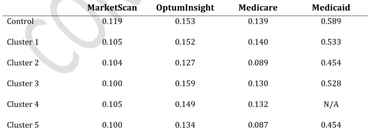
Table 5 shows the variation in input price-adjusted spending, as measured by the coefficient of variation (CV) after adjustment for the predictors in each cluster. For MarketScan, cluster 1 (age and sex) had the largest absolute incremental reduction in variation, from 0.119 to 0.105. Cluster 2 spending — which added health status to age and sex in cluster 1, and was frequently referred to as “baseline” spending — had the largest incremental reduction for OptumInsight. For fee-for-service Medicare, adding a predictor for health status (Clusters 2 and 5) reduced CV substantially. For Medicaid, Cluster 10, which included dummy indicators for states (a proxy for benefit design), reduced the CV most. Across payers, while inclusion of health status resulted in a reduction of the coefficient of variation, that impact was largest for Medicare and OptumInsight. The latter result could follow from greater variability in health status within these populations. One would expect considerable variation in health status among the elderly Medicare population, and among the highly diverse OptumInsight population, which (unlike MarketScan) contains both non-elderly and elderly adults.

Table 5. Coefficients of Variation of Input Price Adjusted Spending by Non-Market Cluster and Population

Control 0.119 0.153 0.139 0.589 Cluster 1 0.105 0.152 0.140 0.533 Cluster 2 0.104 0.127 0.089 0.454 Cluster 3 0.100 0.159 0.130 0.528 Cluster 4 0.105 0.149 0.132 N/A Cluster 5 0.100 0.134 0.087 0.454

(17)

Cluster 6 0.111 0.145 N/A N/A

Cluster 7* 0.105 N/A 0.139 0.533

Cluster 8* 0.103 N/A 0.088 0.454

Cluster 9* 0.100 N/A 0.087 0.454

Cluster 10 N/A N/A 0.088 0.153

Note: An asterisk indicates that those findings are based on a 2-stage OLS regression methodology described earlier. The other estimates are based on a one-stage methodology.

As explained earlier, the subcontractors also analyzed the impact of predictors related to the local health care market. The methods varied slightly, so the results in Table 5 were limited to MarketScan, Medicare, and Medicaid who had nearly identical methodologies. For OptumInsight’s treatment of the impact of market variables, see Appendix 1. MarketScan, Medicare, and Medicaid find that in certain cases market variables either slightly increase or decrease variation in input price adjusted spending. Overall, the impact of market-level predictors utilizing this two-stage process was ambiguous at best.

Finally, PHE explored the relationship of area-level spending across payer populations, focusing on cluster 2 (often referred to as “baseline”) spending, which controls for age, sex, their interaction, partial year enrollment, year dummies, and health status. As Table 6 shows, the private populations were fairly well correlated with one another (+0.632 to +0.663). Otherwise, Medicaid was weakly and often negatively correlated with the private populations and Medicare. Medicare was similarly weakly correlated with the private populations. These findings do not provide clear support for the hypothesis that higher private spending obviates the need for higher public spending (sometimes referred to as a spillover between Medicare and commercial payments), or the alternative that spending varies in a uniform fashion across payers.

Table 6. Correlations of Spending Measures between Populations MarketScan & OptumInsight MarketScan & Medicare MarketScan & Medicaid OptumInsight & Medicare OptumInsight & Medicaid Medicare & Medicaid Total Baseline Spending 0.663 0.112 -0.027 0.081 -0.066 0.141 Input Price Adjusted 0.632 -0.094 -0.140 -0.032 -0.145 -0.015

(18)

Baseline Spending

Note: All HRR means are from the Cluster 2/baseline models which has predictors for partial-year enrollment, age, age*sex, year, and health status. Correlations are pairwise correlations between populations over HRRs.

From these findings PHE concludes that variation was large and that commonly discussed predictors of variation explain some, but not all variation. In fact, between 63% and 85% of variation persisted after accounting for measured health status and market factors.

Utilization

Similar to PHE’s findings for the analysis of spending outcomes, utilization outcomes showed that variation was large, and much remains unexplained and that the populations were even less correlated.

As Table 7 shows, Medicare and Medicaid populations tended to have higher levels of utilization than their private counterparts. Additionally, the MarketScan population tended to have higher utilization than the OptumInsight population, other than for inpatient admissions.

Table 7. Mean Outcomes of Utilization Measures across Populations

Inpatient Admissions 0.005 0.008 0.028* 0.038 Outpatient Visits _0.265 _0.244 _0.585 _0.371 Rx Fills _1.068 _0.506 _2.152 _3.087 ED Visit Days _0.024 _0.015 _0.050 _0.165 Imaging Encounters 0.094 0.069 0.211 0.275

Note: All HRR means are from the baseline/Cluster 2 models which has predictors for partial-year

enrollment, age, age*sex, year, and health status.

*Medicare is the sum of inpatient surgical admissions and inpatient medical admissions, which were reported separately

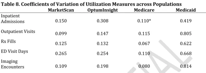
In addition to having the highest average utilization, the Medicaid population also had the highest variation across the various measures of utilization. As shown in Table 8, the OptumInsight population was the next most variable, followed by the MarketScan and Medicare populations who had similar levels of variation.

(19)

Table 8. Coefficients of Variation of Utilization Measures across Populations

Inpatient Admissions 0.150 0.308 0.110* 0.419 Outpatient Visits _0.099 _0.147 _0.115 _0.805 Rx Fills _0.125 _0.132 _0.067 _0.622 ED Visit Days _0.265 _0.254 _0.110 _0.668 Imaging Encounters 0.109 0.198 0.080 0.814

Note: Utilization CVs rely on baseline regressions controlling for partial-year enrollment, age,

age*sex, year, and health status.

*Medicare is the sum of inpatient surgical admissions and inpatient medical admissions, which were reported separately

As Table 9 shows, MarketScan and Medicare also had fairly well correlated utilization outcomes (ranging from 0.411 to 0.699). With the exception of inpatient admissions, MarketScan and OptumInsight had similarly well-correlated outcomes. Medicaid, on the other hand, had low levels of correlations with all of the other populations, with the highest at 0.298.

Table 9. Correlations of Utilization Measures between Populations MarketScan & OptumInsight MarketScan & Medicare MarketScan & Medicaid OptumInsight & Medicare OptumInsight & Medicaid Medicare & Medicaid Inpatient Admissions 0.119 0.674 0.222 -0.045 0.035 0.218 Outpatient Visits 0.706 0.609 0.069 0.526 0.066 -0.052 Rx Fills _0.528 _0.411 _0.230 _0.470 _0.158 _0.157 ED Visit Days 0.665 0.564 0.298 0.581 0.161 0.175 Imaging Encounters 0.397 0.699 0.285 0.333 0.136 0.290

(20)

Note: Utilization measures rely on baseline regressions controlling for partial-year enrollment, age, age*sex, year, and health status. Correlations are pairwise correlations between populations over HRRs. *Medicare is the sum of inpatient surgical admissions and inpatient medical admissions, which were reported separately

Quality

As noted earlier, there were differences between subcontractor methodologies for estimating quality outcomes (for example, whether the measure was expressed as a risk-adjusted rate or an observed-to-expected ratio). For that reason, certain comparisons were not feasible.

PHE could compare the PQI composite results across all studies, and the PSI composite results between the 2 commercial populations and also between the 2 public populations. Additionally PHE could compare the public payers on the IQI composite. For each composite, higher values indicate worse quality.

As shown in detail in Table 10, OptumInsight had higher, and thus worse, PQI outcomes than MarketScan; Medicare and Medicaid were intermediate between the commercial results. For PSI, OptumInsight also has worse outcomes than MarketScan; Medicare was slightly worse than Medicaid. For IQI, Medicaid has worse outcomes than Medicare.

Table 10. Mean Outcomes of Quality Measures across Populations

PQI Composite 0.0004 0.0553 0.005 0.004

PSI Composite 0.003 0.0052 0.949 0.915

IQI Composite N/A N/A 1.005 1.011

Note: Quality measures described in methods section.

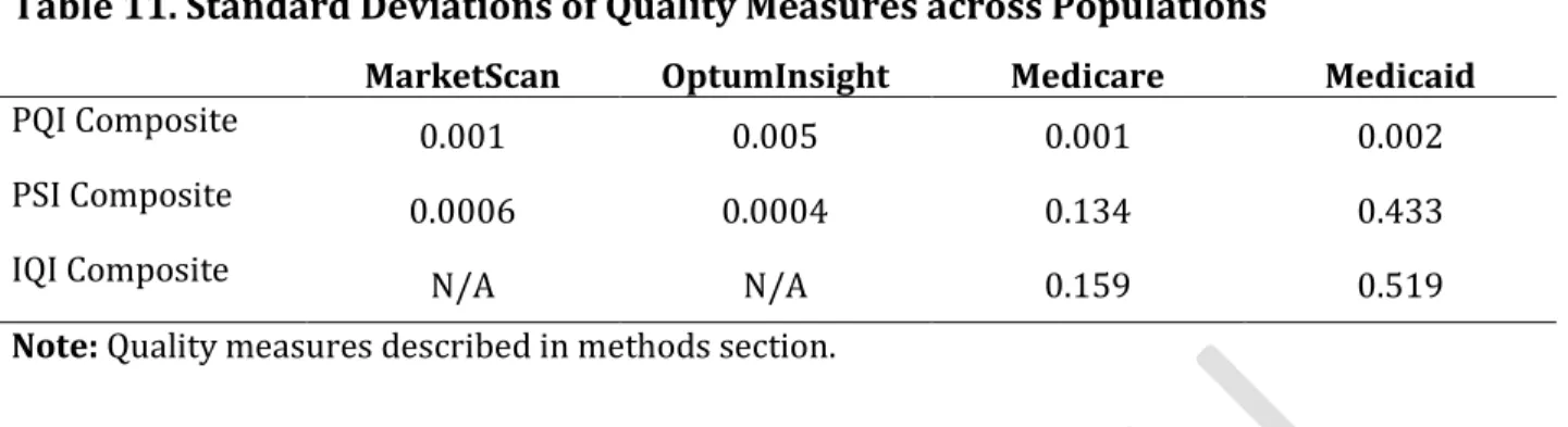
As in the spending and utilization analyses, PHE also compared the magnitude of variation in quality outcomes, where possible. For this task, the IOM requested that PHE evaluate standard deviations, rather than coefficients of variation when comparing geographic variation in quality outcomes. As seen in Table 11, across PQI composite measures of standard deviation, OptumInsight and Medicaid varied most, followed by Medicare and MarketScan. For PSI the private populations had similar deviations while Medicaid’s was much higher than Medicare’s. Finally, Medicaid had much higher variation than Medicare in the IQI composite measure.

(21)

Table 11. Standard Deviations of Quality Measures across Populations

PQI Composite _0.001 _0.005 _0.001 _0.002

PSI Composite _0.0006 _0.0004 _0.134 _0.433

IQI Composite _N/A _N/A _0.159 _0.519

Note: Quality measures described in methods section.

In addition to mean quality outcomes and variation in those outcomes, PHE again analyzed whether these outcomes were consistent across payers. To explore this question, PHE evaluated the correlation of the area effects between populations. As shown in Table 12, the only strong correlation across populations was that between MarketScan and Medicare for the PQI composite of 0.703. Otherwise, quality measures had little relation across payers.

(22)

Table 12. Correlations of Quality Measures between Populations MarketScan & OptumInsight MarketScan & Medicare MarketScan & Medicaid OptumInsight & Medicare OptumInsight & Medicaid Medicare & Medicaid PQI Composite 0.253 0.703 0.230 0.123 -0.017 0.312 PSI Composite 0.050 -0.092 0.020 -0.049 -0.001 0.089 IQI

Composite N/A N/A N/A N/A N/A 0.137

Note: Quality measures described in methods section. Correlations are pairwise correlations between

populations over HRRs.

Variation within Areas

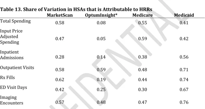
One of the research questions posed by the IOM to PHE was whether variation was occurring at the HRR level, or if it occurs at even smaller levels of geography. To explore that question, PHE performed a random effects regression of spending and utilization at the HSA level, with the random effects at the HRR level.2_{This regression of HSA level}

outcomes with HRR level random effects isolates the share of variation in mean spending and utilization outcomes that is occurring at the HRR level. Those results are reported in Table 13 below. Further, by subtracting that share of variation from 1, PHE can pinpoint how much variation in these outcome measures is attributable to the geographically smaller HSAs. In effect, it provides an upper bound on how much variation a regionally-targeted policy could hope to reduce.

As Table 13 shows, between 40 and 50% of all variation in total spending in HSAs was actually occurring at the larger HRR level, across payers.3_{That share rises for input price}

adjusted spending across public populations. Further, the share of variation in utilization measures occurring at the HRR level was generally greater than one-third. In general, the central tendency was for about 30 to 60 percent of variation to remain even when controlling for HRR characteristics. As all of these statistics show, considerable variation was not explained by those HRR characteristics and was occurring at the smaller HSA level.

2_{Random effects were used to obtain an unbiased estimate of the within-HRR variance, and precluded weighting.}

Fixed effects regressions yielded very similar results. For MarketScan total spending, for example, random effects yielded a value of 0.58, while fixed effects yielded a value of 0.61.

3_{OptumInsight represents an outlier finding based largely on the inclusion HSAs with observations of less than}

200. Excluding those populations leads to an HRR share of HSA variation of 0.33 for total spending and 0.31 for input price adjusted spending.

(23)

This finding suggests that variation occurs within fairly tightly defined geographic areas. Moreover, it is consistent with an even stronger hypothesis, that variation occurs at the level of individual providers – physicians and hospitals. If true, one would expect variation to exist across geographic regions, but geography itself might be incidental to the source of variation. Indeed, any grouping of physicians and hospitals would produce variation in this case. If true, it calls for deeper analysis into the presence and causes of variation across individual physicians and hospitals.

Table 13. Share of Variation in HSAs that is Attributable to HRRs

MarketScan OptumInsight* Medicare Medicaid

Total Spending _0.58 _0.08 _0.55 _0.41 Input Price Adjusted Spending 0.47 0.05 0.59 0.42 Inpatient Admissions 0.28 0.14 0.38 0.56 Outpatient Visits _0.58 _0.59 _0.48 _0.71 Rx Fills _0.62 _0.19 _0.44 _0.74 ED Visit Days _0.42 _0.25 _0.30 _0.67 Imaging Encounters 0.57 0.48 0.47 0.76

Note: Input Price Adjusted Spending controls for age, age*sex, partial year enrollment, year, and health status. Findings based on a random effects model; results are similar with a fixed effects model.

Total Spending

Goal

As noted earlier, the second portion of PHE’s task was to create a measure of total spending, and use that measure to answer two sets of research questions. The first set of research questions focused on how total health care spending varies geographically, and what explains that variation. To answer these questions, PHE, at the request of the IOM, had to incorporate spending by populations not covered in the original population-specific studies: the uninsured and managed care enrollees in Medicare and Medicaid. The second

(24)

research question was to understand whether measures of Medicare quality were better predicted using total spending or Medicare-only spending.

Methodology

To create the estimate of total spending by geographic region, PHE first had to create an estimate of total, unadjusted spending by HRR and then use that estimate alongside additional predictors to quantify how adjusting for additional predictors affected variation in adjusted spending.

Creating an Estimate of Total Spending

To generate the initial estimate of total spending, PHE employed six categories of data:

• _{Medical Expenditure Panel Survey (MEPS) data on spending by the uninsured from}

2007 to 2009

• _{MEPS data on average months spent covered by a given payer}

• _{MSIS Data Cubes data on spending by Medicaid Managed Care enrollees} • _{Census bureau data on age, gender, race/ethnicity, and median income} • _{InterStudy data on population by payer by HRR in 2009}

• _{Data from the three studies (Medicare, Medicaid, and commercial) on:}

o Unadjusted per member per month total spending and input price adjusted

spending

o Means of predictors used in cluster regressions

o Unadjusted per member per month spending for Medicare Advantage

enrollees, from a supplementary analysis obtained by the IOM

o Market-level variables by HRR

More specifically, PHE first estimated spending by the uninsured by HRR, then estimated spending by Medicaid managed care enrollees by HRR. Next, PHE created weights used to add all of the estimates—PHE’s estimates along with the estimates from the earlier studies—to estimate total, PMPM health spending. For commercial spending, PHE used MarketScan, at the Committee’s direction. A limitation of the MarketScan data is that area spending is censored for 53 of 306 HRRs.

(25)

To calculate spending for the uninsured, PHE calculated the average, annual uninsured spending by Census region and MSA status from 2007, 2008, and 2009 (the same years used by the other studies). These eight estimates (four Census regions and non-MSA versus MSA) provide the baseline estimates of uninsured spending on which further adjustments and weights were applied. Next, PHE adjusted those baseline estimates of spending for inflation, using the general CPI and a base year of 2009 and averaging over the three years of data. Then, PHE adjusted those averaged spending estimates using HRR-level estimates of the hospital wage index (HWI) and the geographic practice cost index (GPCI). Each of those adjustments was applied based on a national-level breakdown of inpatient versus outpatient spending to generate updated estimates of input price adjusted spending for the uninsured by Census region and MSA status.4_{(The Kaiser Family Foundation 2011) Those} estimates were then divided by the average number of months per year spent uninsured (about 8.9 from MEPS) to yield per member per month estimates of spending for consistency with other population-specific results. After this step, PHE had generated eight geographically-specific and MSA-status specific estimates of PMPM input-price adjusted spending. Those geographically-specific measures were matched to HRRs by crosswalking census regions to states and states to HRRs based on the Dartmouth Atlas’s crosswalk. At this point, each HRR had geographically appropriate estimates of both MSA and non-MSA, input price adjusted spending. Finally, using data from the Census bureau on the share of HRRs that are urban and rural, PHE created a weighted average of MSA and non-MSA spending within an HRR to create the final estimate of HRR specific spending by the uninsured.5_{See Appendix 2 for estimates of uninsured spending at various stages of the} analysis.

To calculate spending for Medicaid managed care, PHE relied on estimates of: enrollment and total dollars paid for Medicaid HMO enrollees by state. State was the lowest level of geography that PHE could obtain for Medicaid spending. PHE selected HMO enrollees because PHE could be certain that they would not be included in the Medicaid study’s population with “partial” managed care. Using data from the MSIS Data Cubes, PHE downloaded Medicaid HMO enrollment and total dollars paid for those enrollees by state as well as enrollment and total dollars paid for non-HMO enrollees by state. PHE created a per enrollee estimate of dollars paid for these two populations. Then, PHE calculated the ratio of HMO to non-HMO cost per enrollee by state. To control for outliers, those states with ratios above the 90th_{percentile and below the 10}th_{percentile were replaced by the average}

ratio (See Appendix 2 for a breakdown of the ratios). Then, using the same crosswalk from the Dartmouth Atlas as in the uninsured analysis, PHE matched state-specific ratios to proper HRRs. Finally, PHE obtained Medicaid managed care spending by HRR by multiplying those ratios by the Medicaid study’s estimate of fee-for-service Medicaid spending.

4_{HWI: 42.9% (Hospital & Nursing Home); GPCI: 57.1% (Rest)}

5_{The share of the HRR that is urban versus rural was calculated by estimating the urban and rural}

populations by zip code in the 2000 Census. Then, using the Dartmouth Atlas’ crosswalk of zip codes to HRRs, applying those populations to the proper HRRs and calculating their relative shares within the HRR.

(26)

Finally, PHE calculated two measures of total PMPM spending by HRR. The first measure did not adjust for input prices, while the second measure did. Both of these measures corresponded to the “control” cluster used by the population-specific studies; this cluster accounted only for year and partial-year enrollment. In these measures of total PMPM spending, PHE combined the population-specific estimates of PMPM spending by HRR with PHE’s estimates of uninsured and managed care PMPM spending.

To obtain representative estimates by combining PHE’s estimates of spending with the population-specific estimates, PHE needed payer-specific weights. To create these weights, PHE first calculated average months per life per year by payer from MEPS. Because MEPS does not include a monthly measure of enrollment in Medicare Advantage or Medicaid managed care, just of enrollment in Medicare or Medicaid, PHE made the following assumptions. First, PHE assumed that Medicare fee-for-service months were the same as Medicare Advantage months and that Medicaid fee-for-service and managed care months were the same. Therefore, PHE had four estimates of average months per life year from MEPS: 11.7 for Medicare enrollees, 10.2 for Medicaid enrollees, 11.2 for commercially insured, and 8.9 for the uninsured. PHE then multiplied these estimates of average months per patient by payer by the number of patients per payer in an HRR (from the 2009 InterStudy data) to yield total person-months by payer. That estimate was then divided by total person months in the HRR (the sum of the population-specific total months) to yield the weights. Using those weights, PHE calculated the weighted average of PMPM spending across populations by HRR. This procedure yielded an estimate of total, unadjusted per member per month spending and total, input price adjusted spending per member per month, depending on which measure of PMPM spending was used.

Quantifying How Adjustment Affects Variation in Area Spending

In addition to simply estimating total HRR level spending, a goal was to explore how different sets of predictors explain geographic variation in total health spending. Because the focus of the population-specific studies was on input price adjusted spending, PHE used the estimate of total input price adjusted spending by HRR as the starting point. Following the Medicare, Medicaid, and MarketScan methodologies, PHE performed OLS regressions of unadjusted total input price adjusted spending on clusters of predictors, weighting by area population.6_{PHE then estimated the area effects as the sum of the residuals plus the}

population mean. Then, following the other studies, PHE reported the coefficient of variation of these different specifications.

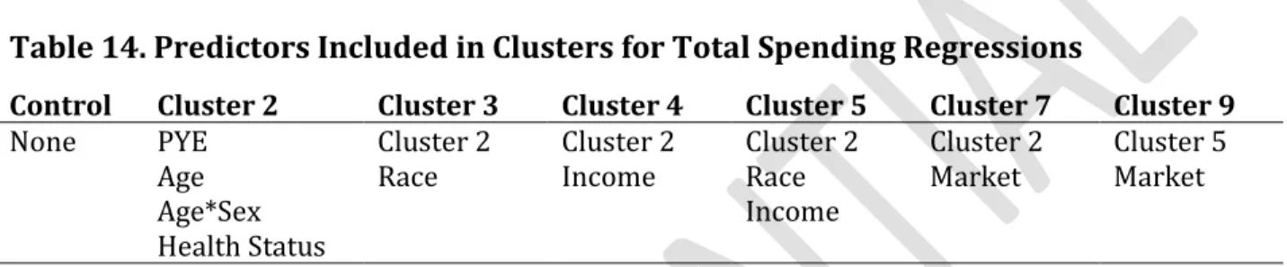
PHE tried to use clusters similar to those employed by the other studies, according to four basic criteria: 1) the policy relevance of the predictors, 2) uniqueness/lack of redundancy of the predictors, 3) the effect size in the population-specific studies, and 4) the availability of consistent measurement of the predictors across payers. For example, PHE included the

6_{PHE weighted areas in its area-level regressions for comparability with the subcontractor regressions, whose}

(27)

malpractice component of the GPCI adjustor as medical malpractice was of some policy relevance. PHE selected only the hospital bed-based estimate of HHI, rather than both versions (including one on the distribution of admissions), because their correlation was greater than +0.8. See Appendix 4 for the full correlation matrix. PHE included percent in an HMO because population-specific regressions found that to have consistently, statistically significant results. And, PHE did not include benefit generosity measures as they were available only for the private population. The resulting clusters are described in Table 14.

Table 14. Predictors Included in Clusters for Total Spending Regressions

Control Cluster 2 Cluster 3 Cluster 4 Cluster 5 Cluster 7 Cluster 9

None PYE

Age Age*Sex Health Status

Cluster 2

Race Cluster 2 Income Cluster 2 Race Income

Cluster 2

Market Cluster 5 Market

Note: Market variables are: specialists/1,000; beds/1,000; HHI bed; % HMO; %Uninsured; Total

Pop; Teaching Hospital; Malpractice GPCI and were provided by the other studies. Race, Income, Age, and Sex come from estimates from the 2000 Census.

Though, wherever possible, PHE mirrored the methods used in the original studies, PHE had to change a few processes. In particular, because the Medicare and Medicaid studies used the complete set of HCCs to estimate enrollee health status, for reasons of parsimony, PHE had to collapse those results into an index of health status. Had PHE not collapsed those disease-specific estimates of health status, our regressions would have been overspecified and difficult to interpret. Further, MarketScan provided a summary index of health status based on Verisk Health DxCG software, so PHE wanted to have a similar index for Medicare and Medicaid. To create this collapsed index of disease-specific estimates, PHE weighted the mean of the predictor for each individual HCC by a formula used to create Medicare Advantage risk scores. (CMS 2008) Under this procedure, each of the specific HCC categories is given a weight, generally between 0 and 1, which expresses its relative importance in predicting the health status (and therefore future health utilization) of beneficiaries. For example, HCC8, lung cancer has a very high weight of 1.053, and HCC 19, Diabetes without complications, has a low weight of 0.162. Those weighted, disease specific estimates are then summed up to create a total index of health status.

Additionally, in order to make the results nationally representative, regressions were all weighted by the population in HRRs. Also, because the health status predictors were specific to a particular study or population, those predictors were additionally weighted by that population’s share of the total HRR population.

(28)

Results

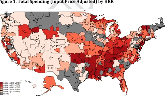
PHE’s estimate of total, per member per month spending by HRR was summarized in Table 15 below. In particular, we find that the estimate of total spending has a somewhat higher coefficient of variation than the estimates produced by the MarketScan or Medicare studies, but was substantially lower than the variation in the Medicaid study (see Table 5 for these other results). Despite the slightly lower estimate, it was clear that there was sizeable variation not only in spending within specific payer populations, but also in total spending. See Figure 1 for an illustration of variation by HRR.

Table 15. Summary of Constructed Total Spending Measure Total Spending

(Unadjusted) (Input Price Adjusted) Total Spending

Mean _$517 _$516

Standard Deviation _100.85 _101.73

C.V. _0.19 _0.20

Notes: These findings reflect the “control” specification which includes only predictors for year dummies and partial year enrollment.

(29)

Table 16 shows the correlation between total spending and payer-specific spending. Total spending is positively correlated with spending for each payer, with correlation coefficients ranging from +0.21 (MarketScan) to +0.63 (Medicaid).

Table 16. Correlation Between Total Spending and Population-Specific Spending

MarketScan Medicare Medicaid

Total Spending

(Input Price Adjusted) 0.21 0.30 0.63

Notes: These findings reflect the control specification which includes only predictors for year dummies and partial year enrollment.

How Do Clusters Explain Variation in Total Spending?

Much like in the population-specific studies, adjustment for commonly discussed predictors explains a meaningful share of variation, but much remains. In particular, adding a control for health status alongside demographic factors like age and sex reduce the coefficient of variation by about 25 percent. Further adjusting for market level factors as well as additional demographic factors only incrementally reduces variation by about five percentage points (from 26% below the control CV to 30% below). These findings were similar to those for the payer-specific populations, as shown in Table 17. This suggests that variation in observed health status explains some of the variation across regions, but much variability remains even after adjustment for health. It should be noted that the health status measures available in this study are not complete – for instance, adding clinical data from medical records and charts might provide additional explanatory power.

Table 17. Impact of Additional Predictors on CV for Input Price Adjusted Total Spending

Control Cluster 2 Cluster 3 Cluster 4 Cluster 5 Cluster 7 Cluster 9

C.V. 0.197 0.148 0.146 0.148 0.146 0.141 0.138

In general, then, the balance of payer specific as well as total spending evidence points to the conclusion that the current set of predictors commonly employed to reduce variation were likely to leave a substantial proportion of that geographic variation unexplained.

(30)

Does Total Spending Predict Medicare Quality Better Than Medicare Spending?

The final research question posed by the IOM was to what extent was Medicare-only spending or total spending a better predictor of measures of quality measures. To test this question, PHE performed OLS regressions (again weighted by population) of area-level quality outcomes (IQI, PQI, and PSI) from the Medicare study on the estimate of total spending as well as on the Medicare study’s estimate of Medicare FFS spending. PHE performed these regressions both with and without the full set of predictors used in the analysis of predictors of total HRR spending. The results of these regressions are summarized in Table 18, below.

Table 18. R-squared Values of Medicare Quality Regression Specifications

IQI PQI PSI _Predictors?Other _{of Interest}Predictor

Specification 1 _0.03 _0.15 _0.01 _N _Total

Specification 2 _0.07 _0.11 _0.04 _N _Medicare

Specification 3 _0.53 _0.73 _0.57 _Y _Total

Specification 4 _0.55 _0.76 _0.57 _Y _Medicare

In the absence of any other predictors (specifications 1 and 2), Medicare spending was generally a better predictor of quality vis-a-vis the IQI and PSI composites than was total spending, but, those differences were modest. The PQI composite was better predicted by total spending. Including predictors (specifications 3 and 4) shows a similar pattern where Medicare spending better predicts the quality measures — now including the PQI composite — for the Medicare FFS population; again, the difference in predictive power based on the spending measure used was modest.

In addition to finding that Medicare spending was generally a better predictor of Medicare quality, it was also interesting to note the sign of those relationships. In particular, as shown in Table 19, the IQI and PQI composites were positively associated with total spending. PSI was also positively associated with total spending, but not at a statistically significant level. Because higher values indicate worse quality of care, higher total spending was associated with lower levels of quality for those measures. However, those findings were not statistically significant when additional predictors of the outcomes were included in the regressions.

On the other hand, Medicare spending in Specification 4 has a negative, significant impact on IQI quality outcomes and a positive, significant impact on PQI outcomes. Again, because a higher quality measure indicates worse quality, this means that additional Medicare

(31)

spending was associated with better IQI outcomes but worse PQI outcomes. See Appendix 3 for a complete reporting of standardized coefficients from regression specification 4. Table 19. Standardized Coefficient on Independent Variable of Interest across Specifications

Medicare Spending Total Spending

IQI Composite _-0.26 _-0.27 _0.18 _0.03

PQI Composite _0.33 _0.34 _0.38 _0.11

PSI Composite _-0.20 _0.01 _0.11 _0.10

Specification ₂ ₄ ₁ ₃

Other Predictors? _N _Y _N _Y

Notes: Predictors include Age, Sex, Age*Sex, PYE, Health Status, Race, Income, specialists/1,000;

beds/1,000; HHI bed; % HMO; %Uninsured; Total Pop; Teaching Hospital; Malpractice GPCI Values in bold are statistically significant at the 5% level.

A striking finding in this table is the variability in the correlation between spending and quality. For example, after adjusting for other covariates, Medicare spending is significantly correlated with IQI and PQI measures of quality, although with different directionality. On the other hand, total spending is uncorrelated with quality after this adjustment.

A number of potential mechanisms might be at work in generating this set of findings, although it is hard to rule any of them out using regionally aggregated data alone. The first is the possibility that Medicare spending is the most highly predictive of quality. This would explain why adding spending from other sources would weaken the estimated correlations. However, one also has to explain why Medicare spending is associated with lower quality for two of the three measures, and higher quality for the third.

Indeed, the overriding feature of these estimates is their extraordinary instability. This is consistent with another explanation, namely that the true relationship between spending and quality is driven by the behavior of individual physicians and hospitals. Suppose, for example, that some providers spend money wisely, while others spend it unwisely. Among the first set of providers, spending might be positively associated with quality. Among the second, it might be negatively associated with quality. The estimated association across regions will depend in general on the fraction of “wise” and “unwise” providers present in high-spending and low-spending regions of the country. These fractions are impossible to predict a priori, so that a number of associations become possible. This could explain the instability of the results across Medicare spending and total spending. Moreover, a given provider might be wise along some dimensions of quality, and unwise along other dimensions of quality. In this case, the sign of the association between quality and spending might vary depending on how quality is measured.

(32)

This simple example demonstrates a more general principle: if the underlying source of variation is not the region, but some other unit, there is no reason to believe that regional associations will be stable or sensible across alternative specifications and measures.

Discussion

This research has confirmed a long-standing fact: significant variation exists in spending across regions of the country, and health status and other measured factors cannot explain all of this variability. We should emphasize that this analysis does not shed light on

whether variation is valuable or harmful. For instance, one could hypothesize that variation represents departures from evidence-based guidelines in some parts of the country; in this case, limiting variation might improve outcomes for patients. Alternatively, one could argue that it reflects efficient specialization in care across the country: some regions specialize in highly intensive forms of care, while others specialize in less intensive forms; in this case, it is preferable for patients in “high-intensity” regions to be treated in this manner, while similar patients residing in “intensity” regions should be treated according to the low-intensity skills of their local providers.

Yet, regardless of whether variation is harmful or beneficial, its presence has important policy implications for the broader health care systems. First, spending across different payers is not perfectly correlated; indeed, there are fairly modest correlations in regional utilization patterns across payers. In other words, a region that spends a great deal of money on Medicare might not spend a great deal of money on Medicaid or commercial insurance. Similarly, regional variation in quality is also not well-correlated across payers; in other words, high-quality Medicare regions might not be high-quality commercial regions. All these facts taken together suggest that providers might be responding

differently to patients with different sources of coverage. Policymakers must pay attention to the particularities of each payer, and regard them as presenting providers with different incentives and patients with different opportunities for care quality.

Second, the evidence suggests that variation exists across relatively small regions, even HSAs. Moreover, some evidence suggests that it extends as far down into the system as individual providers and payers. (Doyle Jr et al. 2010) (Bradford et al. 2001) Yet, many current policy levers work at the state, regional, or county level. If the sources of variation operate beneath these regional groupings, existing policy levers might not be effective. For instance, if individual providers within a county are making different decisions, in spite of facing identical reimbursement schedules, it is unclear that manipulating county-level incentives will significantly limit variation that exists.

Future work in the area of variation in health care might focus less on geography per se, and more on the contributions of individual provider and hospital behavior, and incentives, to the variation that is observed in spending and utilization. This represents a much

different area of focus, as the previous literature has spent a great deal of time and effort quantifying variation across geographic areas in particular. Yet, the instability in

(33)

aligned with the root causes of variation. In our view, the next logical frontier for research on variations must dive into the determinants of individual provider decisionmaking, and their role in delivering appropriate and inappropriate care to patients.